Fast Bayesian methods for genetic mapping applicable for high-throughput datasets

(1)

Fast Bayesian Methods for Genetic Mapping Applicable for

High-Throughput Datasets

Yu-Ling Chang

A dissertation submitted to the faculty of the University of North Carolina at Chapel Hill in partial fulfillment of the requirements for the degree of Doctor of Philosophy in the Department of Biostatistics.

Chapel Hill 2008

Approved by

Advisor: Dr. Fred A. Wright

Reader: Dr. Fei Zou

Reader: Dr. Gary Koch

(2)

(3)

Abstract

QTL mapping is a statistical method for detecting possible gene locations (called

Quan-titative Trait Loci or QTL) and those genes’ effects on the variation in a quanQuan-titative

phenotype, such as the height of a corn plant, etc. QTL mapping has become an important

issue in genetic analysis and has made important contributions to the fields of medicine and

agriculture. Traditional QTL mapping methods scan the whole genome and calculate the

profile likelihood ratios test statistic at each putative QTL location. The maxima of the

test statistics for all putative QTL locations are compared with the genome-wide threshold

to identify the QTL.

In this thesis, we propose several fast Bayesian methods for QTL mapping, which not

only provide direct approximate QTL posterior probabilities at all putative gene locations,

but also offer highly interpretable posterior densities for linkage, without the need for Bayes

factors in model selection. The applications to simulated data and real data show these

methods are highly efficient and more rapid than the alternatives, grid search integration,

importance sampling, Markov Chain Monte Carlo (MCMC) sampling or adaptive

quadra-ture. Our results also provide insight into the connection between the profile likelihood

ratios test statistic and the posterior probability for linkage. The results of these methods

are easy to interpret and have the advantage of producing posterior densities for all model

parameters. We infer the presence of QTL at locations with largest posterior probabilities.

Because of the high speed and high accuracy of these methods, they are highly suitable

for studying high-throughput data sets, e.g. eQTL data sets. The eQTL analysis is a

very important application of QTL mapping to a microarray data set, where thousands of

transcripts are treated as the phenotypes and provides us insight into the natural variation

in gene expression levels. The approach offers highly interpretable direct linkage posterior

densities for each transcript, and opens new avenues for research in this area.

Biologi-cally attractive priors involving explicit hyperparameters for probabilities of cis-acting and

trans-acting QTL are easily incorporated.

We also extend the one QTL Bayesian method to multiple QTL. The advantage of this

(4)

joint effects. Multiple QTL mapping can be computationally intensive, even for our efficient

Bayesian approaches. Thus, a fully Bayesian multiple QTL approach for high-throughput

datasets remains challenging. We investigate a heuristic for conditional search on the

two-location search space that shows promise for identifying the global maximum, and offers

the potential for extended approximate Bayesian approaches.

(5)

ACKNOWLEDGEMENTS

I would like to express my deepest thanks and appreciation to my advisor, Dr. Fred

A. Wright for his tremendous help, patience and encouragement during my Ph.D. work.

Dr. Wright leads me to this interesting quantitative trait loci statistical analysis field. His

sound advice and guidance were invaluable during my research. I have also enjoyed the

inspiring discussions with my coadvisor Dr. Fei Zou who keeps encouraging me to explore

different problems and providing many useful comments and resources during my research.

I am extremely grateful for the kind assistance, generosity, and advice I received from

Dr. Gary Koch at different stages of my study. Thanks to his help and guidance, I can

complete my graduate study for both Master and Ph.D. degrees. I would also like to thank

him for giving me the opportunity to work in the Biometric Consulting Lab. During my

stay in the lab, I have learned so much from the projects, which I participate in. I want to

express my thanks to all members in the lab for encouraging and supporting me during my

studies.

I am grateful to my committee members for investing time and energy discussing ideas

with me. I have benefited greatly from their advice. I thank Dr. Amy Herring for carefully

reviewing my dissertation and providing statistical suggestions in Bayesian perspective. I

also would like to express my thanks to Dr. Daniel Pomp for providing helpful statistical

references and giving useful suggestions from Biological perspective.

This dissertation is dedicated to all my family members for their support and

(6)

LIST OF FIGURES

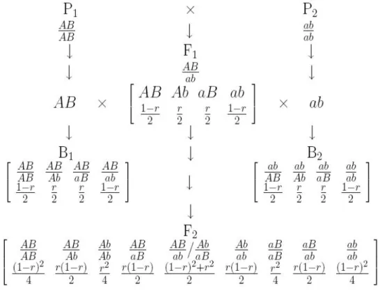
1.1 The breeding process of experimental populations and their recombination rate information, Zeng (2000). . . 4

1.2 Microarray data structure. . . 18

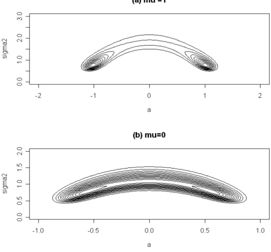
2.1 Contour plot of Laplace approximation for BC data under the null hypothesis: (a) n(sample size)=100,µ= 1 (b) n(sample size)=100,µ= 0. . . 30

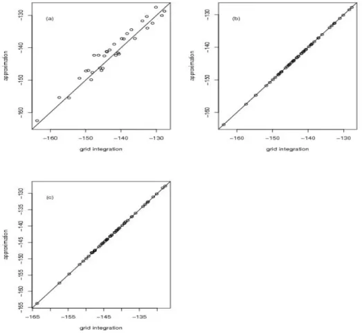
2.2 BC data simulation results for {µ, a, σ2} = {0,0,1} and n = 100 under the null hypothesis: (a)naive null Laplace approximation (b)improved null

Laplace approximation (c) fast nullLaplace approximation. . . 32

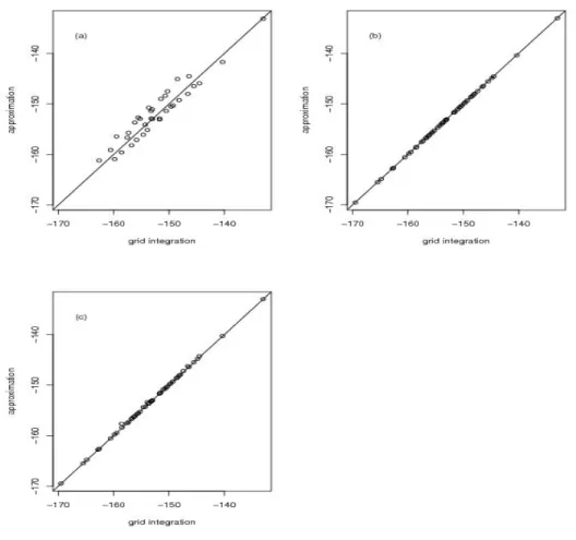
2.3 BC data simulation results for {µ, a, σ2} = {0,0.5,1} and n = 100 under the null hypothesis: (a)naive null Laplace approximation (b)improved null

Laplace approximation (c) fast nullLaplace approximation. . . 33

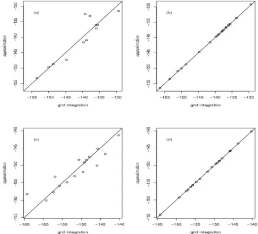
2.4 F2 data simulation results for n= 100 under the null hypothesis: (a) naive nullLaplace approximation (b)fast nullLaplace approximation under{µ, a, d, σ2}=

{0,0,0,1}; (c)naive nullLaplace approximation (d)fast nullLaplace approx-imation under {µ, a, d, σ2}={0,0.5,0.5,1}. . . 35 2.5 Posterior distributions of QTL locations for the chromosome 12 of the F2

data in Naoki et al. 2004. Several methods are applied and compared with the grid search method. The solid curves are for the grid search method, and the red scatter points are for the other methods. . . 63

2.6 The difference of posterior probabilities from each method, compared with the grid search method along chromosome 12. . . 64

2.7 The eQTL plot for budding yeast data. . . 68

2.8 Posterior probability against all genome plot for transcript with the highest cis-acting posterior probability. . . 69

2.9 Posterior probability against all genome plot for transcript with the highest trans-acting posterior probability. . . 70

3.1 The sequential Bayesian QTL method algorithm for detecting two QTL. . 96

3.2 300 simulation results for data generated fromH0,H1 and H2. . . 99

3.3 ROC curve for all three hypotheses. . . 100

(9)

3.4 100 simulation results for detecting QTL locations by using joint Bayesian two QTL method. . . 101

3.5 100 simulation results for detecting QTL locations by using sequential Bayesian two QTL method. . . 103

3.6 Compare 100 simulation results of joint method and sequential method for detecting QTL locations. . . 104

3.7 Posterior distributions of QTL locations on the chromosome 6 and 15 of the BC data from paper Sugiyamaet al.(2001). Joint two QTL Bayesian method is used in this real data analysis. . . 107

3.8 The contour plot of QTL locations on the chromosome 6 and 15 of the BC data from paper Sugiyamaet al. (2001). Joint two QTL Bayesian method is used in this real data analysis. . . 108

(10)

CHAPTER 1

Introduction

In this thesis, we are addressing the problem of detecting the locations and effects of

genes which contribute to the variation of some phenotype. This is called QTL mapping.

Moreover, we also expand the idea of QTL mapping to microarray data and gain insight

into the effect of variations in gene expression levels. This is called eQTL mapping. Most

traditional QTL methods use thelog10 of profile likelihood ratios test statistic (also called

the LOD score in the genetics field) to detect QTL. With these methods, a LOD score for

every putative location is computed. We infer the presence of QTL at locations where the

LOD scores are above some pre-specified threshold.

In most Bayesian QTL methods, it is customary to draw samples of nuisance

parame-ters from the posterior distributions by applying Monte Carlo sampling methods and then

obtain estimates for the unknown parameters based on averaging the samples drawn from

these posterior distributions. In our Bayesian method for detecting one QTL, we propose to

use the Laplace approximation for the integration of the likelihood function with respect to

the nuisance parameters, assuming that the priors of the nuisance parameters are properly

uniform distributed. This method is very fast and accurate compared to all other existing

Bayesian methods. Thus, our Bayesian method is suitable for high-throughput applications

such as eQTL studies. We expand this Bayesian method to detect multiple QTL

simulta-neously and further propose the iterative Bayesian method via the Laplace approximation

for the multiple QTL model. This iterative method has been shown to be relatively fast

and has very high accuracy for detecting multiple QTL locations.

In Section 1.1, we introduce QTL mapping as well as some commonly used

(11)

likelihood-based QTL methods and Bayesian QTL methods in this section. In Section 1.2,

the introduction to microarray data analysis is provided. In Section 1.3, we explain what the

expression Quantitative Trait Loci (eQTL) is, and briefly review some recently developed

eQTL methods.

1.1 QTL Introduction

The history of QTL mapping can be traced back to Gregor Mendel’s study of the shape

of the peas. This classical genetics study involved binary traits, in the sense that the

phenotype has only two outcomes, i.e. the shape of peas is round or not. However, most

natural phenotypes are quantitative, such as heights or yields of crops. This has motivated

the statistical study of the distribution of phenotypes while considering the effects of QTL.

In the 1920s, the development of the chromosome theory and genetic linkage helped us to

understand the effects of genes on phenotypic variation. In the 1990s, biomedical markers

such as Restriction Fragment Length Polymorphisms (RFLPs) and microsatellites were

discovered. Since then, there have been many articles studying traits on different organisms,

such as pigs (Andersson et al. (1994)), maize (Beavis et al. (1991), Stuber et al. (1992)),

mice (Berrettini et al. (1994)) and tomatoes (deVicente and Tanksley (1993)) based on

these linkage maps. By using linkage maps, additional statistical and biological discoveries

have been made.

In the following subsections, we will discuss the experiments that produce backcross and

F2 progeny and the statistical models for QTL mapping, and include literature reviews of

the existing likelihood-based and Bayesian QTL mapping methods.

1.1.1 QTL Experiments

We focus below on the data from experimental crosses: backcross (BC) population and

F2 intercross population. There are also some experimental crosses, such as double haploid and some types of recombinant inbred strains, but we will not introduce them here. The

breeding process of the experimental crosses usually involves choosing two highly divergent

parental strains, each of which is homozygous, e.g. if the genotype of the parental strain is

(12)

strain is aa at this locus, we called it the “low” parental strain. In the following context,

we will focus on the genotypes of their progeny at the same locus. By crossing those two

parental strains, we can produceF1 progeny. TheF1 individuals are heterozygous because

they receive one chromosome from the high parental strain and the other chromosome from

the low parental strain. The chromosome from the high parental strain has genotype Aat

the locus and the other chromosome has genotype a at the same locus. Thus all the F1

individuals have the same genotype Aa at this locus. In order to produce the backcross

population, F1 progeny are crossed back to one of their parents, e.g. the high parental strain withAA. The genotype of the backcross progeny could beAAandAawith the same

probability 1₂. Then two F1 strains are intercrossed to produce F2 progeny. The possible genotypes for theF2 individuals at this locus areAAwith probability 1₄,Aawith probability

1

2, and aa with probability 1 4.

When we consider the genotypes at two loci, the chromosomes of the parental strains

during meiosis (the formation of the sex cells) may cross over and recombine. This affects

the joint distribution of the genotypes at two loci. The probability of recombinationr(also

called the recombination rate or recombination fraction) is calculated by Haldane’s map

function here.

r= 1 2(1−e

−2x₎_. _(1.1)

In this formula, x is the map distance between two loci, the expected number of

crossovers between two loci, and it is described in unit: Morgan (M). The

recombina-tion rate r increases from 0 to 0.5, as the map distance between the loci increases from 0

to∞.

When using Haldane’s map function, “no crossover interference” is assumed, which

means that for more than two markers, the recombination event between any two of them

is independent of the recombination event between any other non-overlapping two markers.

Many other map functions have been proposed, for example, the Morgan map function and

Kosambi map function (Ott (1991)) are also very popular, and are used under different

assumptions in a more complicated biological process.

(13)

Suppose that the high parental line (P1) has genotypesAAandBBat two loci in which we are interested. The other low parental line (P2) has genotypes aa and bb at the same

two loci. Figure 1.1 shows the cross process of backcross progeny and F2 progeny. It also

shows the distribution of genotypes at these two loci, assuming that the recombination rate

between the two loci isr. In this Figure, B1 shows the distribution of the genotypes of the

backcross progeny, which are from the crossing of the F1 population and the high parental

strainP1. B2 shows the other distribution of the genotypes of the backcross progeny, which are from the crossing of the F1 population and the low parental strain P2. The last line shows the distribution of the genotypes of F2 progeny, which are from the intercross of theF1 strain. The purpose of the cross process is to increase the genetic variability of the progeny strains and therefore allows us to detect the possible genes for the variation in the

quantitative phenotype.

(14)

1.1.2 QTL Statistical Model

Suppose that yi (i = 1,2,· · ·, n) represents the ith individual’s phenotype and also assume that the QTL are located somewhere between the markers in our model. We intend

to find the locations and effects of QTL given the markers’ genotypes, the markers’ locations,

and the phenotypes of all individuals.

One QTL model:

First, we consider the most simple model: the one QTL model for backcross progeny. The

following equation represents how one QTL genotype affects the distribution of phenotypes:

yi =µ+a·gi(x∗) +i, (1.2)

whereµis the intercept, ais the additive effect of the QTL, x∗ signifies the location of the

unknown QTL, gi(x∗) represents the QTL genotype for the ith individual,gi(x∗) = 1 or -1

if the QTL genotype is Aa(heterozygote) oraa (homozygote), andi is the environmental

variation with a distribution ofN(0, σ2).

Similarly, the one QTL linear model of phenotypes yi for the F2 population is shown

below:

yi =µ+a·gi(x∗) +d·(1− |gi(x∗)|) +i, (1.3)

where a and d are the additive and dominance effects for the QTL, gi(x∗) equals 1 if the

QTL genotype of theith individual is AA, 0 if it isAa, and -1 if it is aa, andµ and i are

defined the same usually as before in the backcross model.

In the above two models, the phenotypes of the individuals follow a mixture normal

distribution since gi(x∗) is unobserved if x∗ is not located at one of the marker locations.

The variance σ2 is defined as a constant. Multiple QTL model

Some phenotypes are affected by more than one QTL, so multiple QTL models are discussed

here. We assume that these QTL act additively, and there may be some interactions between

(15)

them in our model.

The equations below show two QTL models for the backcross and F2 populations,

re-spectively, under the condition that two QTL act additively and independently.

For a backcross population:

yi =µ+a1·gi(x∗1) +a2·gi(x∗2) +i, (1.4)

where a1 and a2 are the additive effects of two QTL, respectively; x∗₁ and x∗₂ specify the locations of two QTL on the chromosome.

For aF2 population:

yi =µ+a1·gi(x∗1) +a2·gi(x∗2) +d1·(1− |gi(x∗1)|) +d2·(1− |gi(x∗2)|) +i, (1.5)

whered1 and d2 are the dominance effects of two QTL, respectively.

If two QTL exhibit deviation from additivity (i.e. there is an interaction effect between

two QTL), called epistasis, the model will become more complicated. The following equation

is the two QTL model with the pairwise interaction for a backcross population:

yi =µ+a1·gi(x∗1) +a2·gi(x2∗) +δ·gi(x∗1)·gi(x∗2) +i, (1.6)

whereδ is the epistasis effect between two QTL.

For the kQTL problem, the model can be generally expressed as:

yi=µgi1,gi2,···,gik+i, (1.7)

wheregi1, gi2,· · ·, gik are the joint QTL genotypes for theith individual,µgi1,gi2,···,gik

rep-resents the phenotypic mean ofyiif theithindividual has QTL genotypes: gi1, gi2,· · ·, gik, i follows N(0, σ2). For the backcross population, the maximum number of unknown pa-rameters is 2k_{+ 1 and the maximum number of unknown parameters for F2 population is}

(16)

1.1.3 Likelihood-Based One QTL Methods

The quantitative inheritance was discovered in the 19th century and arise via the

seg-regation of multiple genetic factors, modified by environmental effects. In this section, we

will describe some major one QTL likelihood-based methods that have been used since the

early 19th century. For each method, we will discuss the main idea, its advantages and its

possible disadvantages.

Binary traits were first described by Gregor Mendel through extensive experiments with

the breeding of peas; he found that the shape of peas is either round or wrinkled, i.e. it is a

binary trait. However, there are also many other traits which exhibit quantitative variation

and which require further investigation.

Thoday (1961) addressed the idea of using genetic markers for identifying multiple genes

that control the quantitative variation of some phenotypes. This idea are examined

exper-imentally after biochemical markers such as Restriction Fragment Length Polymorphisms

(RFLPs) and microsatellites were discovered. The advantages of using biochemical markers

to characterize QTL are their phenotypic neutrality, highly polymorphic properties, and

their abundance in the genome.

The following methods are based on whole genome analysis:

Analysis of Variance (ANOVA)

Soller et al. (1976) used ANOVA for QTL analysis. The phenotypes of individuals are

grouped by the genotypes of the markers. Instead of testing the significance of QTL at

some putative locus, we compare the group means between two genotypes of the marker.

If the QTL is tightly linked to this marker, then grouping phenotypes according to the

genotypes of this marker is essentially the same as grouping phenotypes according to the

genotypes of the QTL.

Analysis of variance (ANOVA) is a simple and naive method that permits very fast

com-putation. However, there are some drawbacks with this method. First, we can’t estimate

the precise location of the QTL. ANOVA only shows which marker is closest to the QTL.

Second, when the markers are not dense enough, the linkage between a QTL and its closest

marker is weak. The power to detect the presence of a QTL is quite small. Third, if we

(17)

estimated the QTL effect by the effect of its nearest marker, we would underestimate its

effect; see Lander and Bostein (1989).

The Maximum Likelihood Method (MLE)

To avoid the drawbacks of ANOVA, Weller (1986), Weller (1987) and Simpson (1989)

con-sidered the difference between QTL and markers. They include the recombination rate r

between a QTL and its markers in the model and test every marker one after another to

find whether there is a QTL close to any of them. This method works via the following

process: taking the backcross population as an example, it assumes that the individuals

with QTL genotype AA have phenotypes distributed as N(µA, σ2), and the individuals with QTL genotypeAahave phenotypes distributed as N(µa, σ2).

For those individuals with the genotype AA at the marker which you are testing, the

phenotype has the following distribution:

yi ∼(1−r)×N(µA, σ2) +r×N(µa, σ2).

But if the individuals have the genotype Aaat the test marker, the phenotype follows the

distribution below:

yi ∼r×N(µA, σ2) + (1−r)×N(µa, σ2).

yi is the phenotype of the ith individual. r is the recombination rate between the

QTL and the marker you are testing. The method uses the EM algorithm to find the

maximum likelihood estimates (MLE) for the unknown parameters. One way we can test

H0:r = 1₂ vs. HA:r6= 1₂ with the LOD score:

LOD=−log10L(ˆµA,µˆa,σˆ

2_{, r}₌ 1 2) L(ˆµA,µˆa,σˆ2,rˆ)

.

Alternatively, we calculate the LOD score for each marker locus to test whether there is

a QTL around the marker and for eachr, the formula of LOD score for testingH0 :µA= µa vs. HA:µA6=µa is:

LOD(r) =−log10L(ˆµA= ˆµa,σˆ 2₎ L(ˆµA,µˆa,ˆσ2)

(18)

The second test is a special case of the first one. The LOD scores are then compared to

a genome-wide threshold to infer the presence of a QTL. This method considers the fact

that the LOD score is computed between markers. However, when using this method it is

hard to combine the results for testing each marker and get a single estimation of the QTL

location and effect.

Interval Mapping

Lander and Bostein (1989) introduced a significant improvement on QTL analysis by using

the flanking markers to detect a QTL in experimental populations; this method is called

“interval mapping”. In this paper, they assume that there is no crossover interference

for any pair of markers on the chromosomes under study and the phenotype is normally

distributed. One has the information on the markers’ locations and markers’ genotypes. A

backcross population is used here to explain this method. The phenotype of each individual

follows a normal distribution with the mean equal to µA orµa depending on whether the

QTL genotype isAAorAa, and the varianceσ2 is defined as a common constant.

In a backcross population, there are two kinds of QTL genotypes and four possible

genotypes at two flanking markers. Suppose the map distance between flanking markers is

d. The map distance between the QTL and the left marker is dL. According to Haldane’s

mapping function, the recombination rate between two markers is r = 1₂(1−e−2d). The recombination rate between the QTL and the left marker is rL = 1₂(1−e−2dL). And the recombination rate between the QTL and the right marker is rR = 1₂(1−e−2(d−dL)) = (r−rL)(1−2rL). We calculate the conditional probability for two possible genotypes of the QTL, given the flanking marker genotypes, by using a recombination rate. The results

are shown in Table 1.1.

Suppose that for individuals with QTL genotypesAA, their phenotypes are distributed

asN(µA, σ2), and for individuals with QTL genotypesAa, their phenotypes are distributed asN(µa, σ2). Then for any given putative QTL locationx, we can calculate the conditional probability assuming that the QTL genotype is AA for the ith individual (i = 1,· · · , n), given its flanking markers, and we note it as Pi(x). Then the ith individual’s phenotype

follows a mixture normal distribution:

(19)

Table 1.1: The conditional probability of a QTL genotype given two flanking makers’ geno-types

is

marker genotype QTL Genotypes

left right Aa AA

Aa Aa (1−rL)(1−rR)/(1−r) rLrR/(1−r) Aa AA (1−rL)rR/r rL(1−rR)/r AA Aa rL(1−rR)/r (1−rL)rR/(1−r) AA AA rLrR)/(1−r) (1−rL)(1−rR)/(1−r)

yi∼Pi(x)×N(µA, σ2) + (1−Pi(x))×N(µa, σ2)

.

For each fixed location x, we use an EM algorithm to maximize the joint likelihood

function and get the estimation for the unknown parameters (See Dempster et al. (1977)).

Considering the null hypothesis that there is no single QTL on the chromosome, the LOD

scores are calculated and plotted against x. The formula of LOD score for test H0 :µA= µa vs. HA:µA6=µa is:

LOD=−log10L(ˆµA= ˆµa,ˆσ 2₎ L(ˆµA,µˆa,σˆ2)

.

We infer the presence of a QTL, if the LOD score at this position exceeds the genome-wide

threshold.

The interval mapping method and the above MLE method are not identical. In the MLE

method, we only consider the recombination rate between the QTL and one marker. But

with interval mapping, we consider the distribution of QTL’s genotype, given two flanking

markers’ information. The interval mapping method can give a precise estimate of the

location and effect of a QTL. Therefore, many QTL statistical methods in the 1990s are

the extensions based on the interval mapping methods. However, it has the drawback: it

(20)

1.1.4 Likelihood-Based Multiple QTL Methods

Many traits may be influenced by multiple genes, so one QTL model is not sufficient

to deal with this situation. We need to develop more complicated models because using

one QTL model to detect multiple QTL data may fail to identify and estimate the

multi-ple QTL locations. The detection power therefore is compromised and estimations of the

QTL locations and their effects will be biased (Lander and Bostein (1989); Knapp (1991)).

Sometimes “ghost QTL” may appear, in the sense that if there are two QTL on a

chromo-some evaluated with one QTL mapping method, you may detect a QTL located chromo-somewhere

between two true QTL locations instead of detecting either one of them (Haley and Knott

(1992); Martinez and Curnow (1992); Yi (2005)).

Multiple QTL can be mapped more accurately and more efficiently with a multiple QTL

model. We will discuss three main likelihood-based methods for multiple QTL mappings:

multiple linear regression, composite interval mapping (CIM) and multiple interval mapping

(MIM).

Multiple Linear Regression Analysis

This multiple QTL method is an extension of the ANOVA method for one QTL model.

In this method, the phenotypes of individuals are regressed on the markers’ genotypes.

The basic idea is that the effects of a QTL will be partially absorbed by linked markers

(Stam (1991)). Cowen (1989) used stepwise selection and backward deletion techniques to

select a class of markers, which are linked to a QTL. More recently, Doerge and Churchill

(1996) described using forward selection and permutation tests to determine the number of

markers in the model. However, when the distances between markers and QTL are large,

only a small part of the QTL effect is absorbed by the markers. The power of detection

thus becomes very small. We cannot estimate the precise locations and effects of a QTL

using this method.

Composite interval mapping

With one QTL interval mapping, the likelihood function for a single QTL is assessed at

each putative location on the chromosome. However, a QTL located somewhere else on

the genome can have an interference effect. Jansen (1993), Zeng (1993) and Zeng (1994)

(21)

independently proposed the idea of combining interval mapping with multiple regression on

markers’ genotypes. Zeng (1994) named this method Composite Interval Mapping (CIM).

The method is achieved by fitting one QTL interval mapping method and using part of the

markers as co-factors to eliminate the effects of additional QTL. By fitting other genetic

markers in the model as a control, it confines the test of one QTL to a region, which changes

the problem from a multi-dimensional search to a one-dimensional search. Compared to

one QTL interval mapping, CIM improves both the sensitivity and accuracy by including

the markers, which may absorb the effects of other QTL. The parameters in the model

are estimated by the expectation/conditional maximization (ECM) algorithm (Meng and

Rubin (1993)).

The main challenge in this model lies in determining which markers to use as regressors.

Jansen and Stam (1994) used backward deletion to pick up the subset of most significant

markers with Akaike’s Information Criterion (AIC). Zeng (1994) recommended that one

include all the markers except those that are within 10 CM of the putative location.

Multiple interval mapping

If there are multiple QTL in the model, Lander and Botstein suggest detecting QTL one

by one, i.e. they fix the position of the first QTL, then look for the next QTL location.

This is a forward selection procedure (Miller (1990)). However, there is the drawback of a

“ghost QTL” effect, in the sense that if there are two or more linked QTL, then interval

mapping often gives a maximum LOD score at a location between the two QTL; see Haley

and Knott (1992).

Kao et al. (1999) extend one QTL interval mapping model to a multiple QTL interval

model. They use multiple marker intervals simultaneously to detect multiple putative QTL

in the model. This method uses the general formulas derived by Kao and Zeng (1997) to

obtain maximum likelihood estimates (MLEs) for the parameters. Compared with the

re-gression method, this method gives accurate and precise locations and the effects of multiple

QTL. However, the selection of the QTL involves multidimensional search, which is very

(22)

1.1.5 Bayesian QTL Methods

Likelihood-based QTL methods detect the locations and effects of QTL mainly by

max-imizing the likelihood and evaluating the presence of QTL by using the LOD score. When

computing confidence intervals, likelihood-based methods do not properly account for

un-certainties in the parameters. With Bayesian methods, the prior information is incorporated

into the analysis and the inferences are based on the marginal posterior distributions of the

parameters, which are easy to interpret.

Satagopan et al. (1996) applied the standard Markov chain Monte Carlo (MCMC)

method to map a given number of multiple QTL on the genome. MCMC is a Bayesian

method commonly used to approximate a multi-dimensional integral of the likelihood

func-tion, which has no closed form. We generate a sequence of samples from the joint conditional

probability distribution to get the integral. For the posterior probability of the parameter

we are interested in, we sample each parameter from its conditional distribution given the

rest of the parameters. The samples of the parameters are generated sequentially until the

chains converge. Satagopanet al.(1996) used Gibbs sampling as well as Metropolis-Hastings

algorithms to sample unknown parameters and missing data from their joint posterior

dis-tribution. The parameters were inferred based on their marginal posterior distributions,

which can be obtained from the joint posterior distribution by integrating over the other

unknowns. It is hard to get the exact integrations over multiple parameters, however, a

Monte Carlo approximation is quite feasible for estimating the integrations. In the paper,

the probability intervals for locations of multiple loci and their effects are discussed. This

method accounts for the uncertainties in the parameters by considering the marginal

pos-teriors, which average over such uncertainties in the parameters. The present paper also

discusses the number of loci affecting the trait of interest. We estimate the number of QTL

by fitting various models with different numbers of QTL, then we use a Bayes factor (Kass

and Raftery (1995)) to compare these models.

The above Bayesian inference is complicated when the number of QTL is unknown.

Essentially, the parameter space is the product of the spaces of different numbers of QTL.

Most conventional techniques can’t be applied. Green (1995) proposed using reversible jump

(23)

Markov chain Monte Carlo alogrithms specifically for such problems. This method combines

the traditional MCMC algorithm with Metropolis-Hasting (Hastings (1970), Metropolis

et al.(1953)) for jumping between different number of QTL. Satagopan and Yandell (1996)

used a reversible jump MCMC to fit a multiple QTL model by including the number of

QTL as unknown parameters. The locations, effects, and number of QTL can be estimated

from the samples. Their application to the Brassica flowering data (Satagopan and Yandell

(1996)) shows similar results compared to the results obtained using Bayes factors

(Sa-tagopan et al. (1996)). Because the reversible jump MCMC algorithm is very general and

widely applicable, many effective approaches for detecting multiple (non-)epistatic QTL

are based on it in different experimental populations or in pedigrees (Stephens and Fisch

(1998); Sillanpaa and Arjas (1998); Thomaset al.(1997); Yi and S. (2000); Gaffney (2001);

Yi and Xu (2002); Yiet al.(2003)). However this method also has its drawbacks: it is very

poor to mix the chain for updating QTL locations and it is very slow for chain convergence.

The Bayesian approach above provides a sensible inferential framework for multiple

QTL mapping. But it suffers from an intense computational burden. Berry (1998) has

proposed another Bayesian model, which is also a Markov chain Monte Carlo method, but

one with moderate computational speed. Usually the joint likelihood function is integrated

over all other unknown parameters to get the posterior distributions of the number and

the locations of QTL. When the number of parameters is large, the computation becomes

very intensive. In Berry (1998), the ease of the computational burden was achieved by

several approximations. Berry (1998) uses a first order approximation of the likelihood

function, and the Laplace approximation to estimate the posterior distribution on the whole

genome. The computation is improved through these approximations. Gibbs sampling is

used to generate samples from the approximated posterior distributions. The number and

the locations of QTL are inferred from the samples. The strength of this method is the

moderate computation speed achieved by using fast approximations. However, this method

is applied only in backcross populations and the accuracy of this approximation still requires

further investigation.

Yi (2004) improved the efficiency of the reversible jump Markov chain Monte Carlo

(24)

QTL. This method is based on a composite space representation of the problem, which was

developed by Carlin and Chib (1995). It provides a new viewpoint on the model selection

problem. The advantage of this new method is that it allows Markov chain Monte Carlo

simulation to be performed on a space of fixed dimension, thus avoiding the complexities

of reversible jump technique. The Bayesian approach is finally simplified. The composite

model space approach is extended to include epistatic effects in the model (Yiet al.(2005);Yi

et al. (2007a)). They developed a computationally efficient Markov chain Monte Carlo

algorithm using a Gibbs sampler and Metropolis-Hastings algorithm to study the posterior

distribution of the parameters.

There are also some other Bayesian methods that can be used to calculate the posterior

probabilities: numerical grid search integration, adaptive numerical integration, and

impor-tance sampling. Numerical grid search integration is a method that is used to approximate

the integral function with no closed form by using a set of grid points. We obtain those grid

points in a user-defined size domain for each nuisance parameter. We also know that the

domains of the nuisance parameters for the integral likelihood is on the space Ω, and Ω can

be arbitrarily large. If we truncate Ω to a reasonable rectangle size such that the likelihood

would be very small outside of the rectangle, numerical grid search integration can divide

this rectangle into many small cubes by the grid points we define, and get the integral

value for each small cube. Then we can add up all the integral values on these small cubes

to find the approximate value for the integral likelihood function. If the cubes are small

enough, we should get a good approximation for the integration of the likelihood function.

The disadvantage of this method is that it has a computationally intensive problem, so it

is hard to apply it to high-throughput applications.

Adaptive numerical integration is a method used to approximate the integral over a

multidimensional finite range by a recursive adaptive method, which divides the interval

into two and compares the values given by Simpson’s rule and the trapezium rule (Venables

and Ripley (1994)). In R software, the “adapt” command in the package “adapt” is used

to apply this method. It works well when models have only a few nuisance parameters.

But when we apply this method to a model with many nuisance parameters or to a very

complicated model, the adapt command in R software is very computationally intensive,

(25)

and can crash easily.

Importance sampling is a Monte Carlo method used to approximate an integral function

by the average of ratios of likelihood density to the proposal density. A set of samples are

evaluated to obtain the average ratios. We have to find a good proposal density, which is

easy to simulate and “near” the density we want to integrate.

Sometimes, the traits we are interested in are binary responses. With most existing QTL

mapping methods, the linkages between markers and QTL are tested with a simple

chi-square test because of the binary traits. Xu (1996) proposed a composite interval mapping

method, which treats a binary trait as the outcome from an underlying normally distributed

liability. The quantitative liability is modelled by the usual QTL mapping method, since it

is quantitative and continuous. Huang et al.(2007) have proposed a new Bayesian method

which combines the unified Bayesian method and the liability model for studying binary

traits. This Bayesian method uses all the markers on the entire genome simultaneously.

Huanget al.(2007) developed the method for the case in which the QTL are located at the

observed markers, and for the case in which QTL are located between markers. If the QTL

are located between markers, the first method will lead to biased estimations. However, if

the markers are dense enough, the first method will be quite accurate and could save much

computation.

1.2 Microarrays Introduction

Microarray technology has become very popular in recent years and plays an increasingly

important role in biomedical research. Disruptions or changes in genes can cause disease or

morphological anomalies. By using microarray technology, we can detect changes in gene

expression and prevent the genetic defects in advance. With microarray technology, we can

measure thousands of genes simultaneously for different types of cells or tissues and use

gene expression to describe their DNA information. Many statistical problems have arisen

recently in the use of microarray data. Well-developed statistical methods that can assist

us in locating the genes of interest are urgently needed.

A microarray data structure is shown in Figure 1.2 on the next page. In Figure 1.2,

(26)

genes. Each row in the gene expression matrix represents the expression values for each

gene with respect to all samples. Each column in the gene expression matrix represents the

expression values of each sample for all genes.

Spotted cDNA microarrays and oligonucleotide arrays (Affymetrix, Santa Clara CA)

are two of the most commonly used gene expression arrays. In spotted cDNA microarray

experiments, the ratio of red and green fluorescence intensity for each spot (gene) is

in-dicative of the relative abundance of the corresponding DNA probe in the two nucleic acid

target samples. The red (R, Cy5) labeled and green (G, Cy3) labeled mRNAs represent test

and control samples, respectively. Probes are cDNA fragments attached on a solid support

(a nylon or glass slide). The process works like this: first, the red and green labeled RNA

samples are mixed and hybridized to the microarrays, which the supplier has spotted with

cDNA from thousands of genes, each spot representing one gene. After hybridization, the

red or green fluorescent signal from each spot is determined and the ratio of red to green is

the primary measurement considered. If one gene has a signal closer to red, this means that

gene is expressed at a higher level in the test sample than in the control sample. Newton

et al.(2001), Dudoit et al.(2002) and Leeet al.(2000) represent some early representative

papers for two-color microarrays.

(27)

(28)

In oligonucleotide arrays, instead of using one probe per gene, 11 to 20 probes are used to

represent each gene (Lockhartet al.(1996)). Each probe represents a unique DNA fragment

of one gene so a group of probes identifying a gene is called a probe set; in principle, one can

obtain a better estimate of the expression level for the gene on probe-set arrays than for the

gene on single-probe arrays. In Affymetrix technology, there is a perfect match (PM) probe

for the target DNA sample, as well as a corresponding paired ”mismatch” probe (MM).

This mismatch probe contains only a single base change in the nucleotide located in the

middle of the 25-base probe sequence; it is designed to measure non-specific hybridization

as well as provide the information on background and cross-hybridization (Lipshutz et al.

(1999)). A perfect match probe and its mismatch probe are called a probe-pair.

There are some differences between these two arrays. For spotted cDNA microarrays,

one probe represents one gene; each array has two target samples or one target sample, and

one reference sample; probe length on spotted cDNA microarrays varies. For oligonucleotide

arrays, there are 11-20 probe-pairs per gene, each array has one target sample, and probe

length is fixed with 25-mers (base pairs).

Statistical problems in this field involve microarray pre-processing like image analysis,

background correction, expression quantification, normalization and quality assessment.

There are also interesting problems when one is comparing two different conditions, like

normal/disease, control/treatment, or when one is comparing more than two different

con-ditions with microarray data. Statistical methods, like estimates and hypothesis testing, are

applied to solve these problems. Exploratory analysis using microarrays is also important.

Let us say we need to find a group of genes for a novel disease by using clustering or

pro-jection methods. There are also many other statistical problems and developed statistical

methods in microarray analysis, which is not the focus in this dissertation and will not be

discussed here.

1.3 eQTL Introudction

Quantitative geneticists are now interested in detecting expression quantitative trait

loci (eQTL) for gene expression abundances because transcript abundances are considered

to correlate with some important phenotypes. Transcript abundances can be treated as

(29)

a surrogate of phenotypes (Schadt et al. (2003)). eQTL methods have been developed

to identify major-effect eQTL for transcripts by combining quantitative trait loci (QTL)

mapping methods with microarray data, and “eQTL” are statistically significant peaks

in a genome-wide scan for linkage analysis. In eQTL analysis, the experimental design

is very similar to traditional quantitative trait loci analysis. The difference is that the

expression values for the gene transcripts are treated as the phenotypes, so one must analyze

thousands of phenotypes in eQTL analysis. Because of this difference, traditional QTL

statistical methods, designed for testing (at most) tens of phenotypes, cannot be easily

applied. Experimental design issues need to be addressed to handle these large data sets

and new statistical methods are still being evaluated.

Bremet al.(2002) used the Wilcoxon-Mann-Whitney method for testing the significance

of the linkage between each marker and transcript. This test has shown some promise in

important biological situations and the resulting p-values for some transcripts are sufficiently

small. Schadt et al. (2003) have used a traditional QTL interval mapping method for

analyzing maize, mouse and human data sets. This likelihood-based approach can be used

to obtain transcript-specific significance profile likelihood curves. However, those methods

are still not well refined for problems like the potential increase in type I error by testing

multiple markers, or power loss. Kendziorski et al. (2006) have proposed a

Mixture-over-Markers (MOM) model to localize eQTL and have controlled the false discovery rate without

sacrificing power. This method is a marker-based model. If the marker density is not

sufficiently dense, the results for loci between markers may have some bias. New statistical

methods are still needed to evaluate the eQTL data and optimize the test results.

Many eQTL studies based on the statistical methods mentioned above or some other

very simple statistical methods have been published for many creatures, e.g. yeast (Brem

et al.(2002); Yvertet al.(2003)), eucalyptus (Kirstet al.(2004)), mice (Schadtet al.(2003);

Bystrykh et al. (2005); Chesler et al. (2005)), rats (Hubner et al. (2005)), maize (Schadt

et al.(2003)) and humans (Morleyet al.(2004); Monkset al.(2004); Hubneret al.(2005)).

For those main regulated transcripts, results reported in several papers show that up to

one-third of the significant genes are cis-acting, which means the gene expression values can be

(30)

trans-acting, which means that the gene expression values are regulated by other physical gene

locations. Most of the cis-acting genes explain a greater proportion of expression variation

than trans-acting genes. Trans-acting genes usually explain little variation individually, but

we have more of them. This is similar to our expectation that DNA variation can affect a

large portion of gene expression for that gene.

In summary, eQTL analysis has the potential to impact biological endeavors in a wide

range of biomedical and agricultural fields. Applying traditional QTL methods to

microar-ray data also gives us insight into gene networks, as well as their evolution. Because of

the computational demands in eQTL analysis, the current statistical methods are not

suit-able for this high-through application. Well-developed and fast statistical methods are still

needed to handle thousands of phenotypes efficiently.

1.4 Thesis Summary

In Chapter 1, we introduced QTL mapping and summarized some existing methods

for detecting QTL. We also provided a brief introduction to microarray data and eQTL

analysis.

In Chapter 2, Bayesian methods via the Laplace approximation for detecting single

QTL are proposed. They can be easily applied to a backcross (BC) population and anF2

intercross population. They can also be trivially extended to double haploid and other types

of recombinant inbred strains. The applications to simulated data and real data demonstrate

the high speed and high efficiency of these methods compared to alternative grid search

integration, importance sampling, MCMC and adaptive quadrature methods. Our results

also provide insight into the connection between the LOD curve and the posterior probability

for linkage. In the application of our Bayesian method, we extend our approximate Bayesian

linkage analysis approach to the expression quantitative trait loci (eQTL) model, in which

microarray measurements of thousands of transcripts are examined for linkage to genomic

regions. This approach uses the Laplace approximation to integrate over genetic model

parameters (not including genomic position), and has been fully developed for different

types of recombinant inbred crosses. The method is much faster than the more

commonly-used Monte Carlo approaches, and thus is suitable for the extreme computational demands

(31)

of eQTL analysis. The approach offers highly interpretable direct posterior densities for

linkage for each transcript at each genomic position. Biologically attractive priors involving

explicit hyperparameters for probabilities of cis-acting and trans-acting QTL are easily

incorporated.

In Chapter 3, we extend the one QTL Bayesian method via Laplace approximation

method to the Bayesian method of detecting multiple QTL simultaneously. This joint

multiple QTL Bayesian method has the advantage of providing the posterior probability

at putative QTL locations and can detect QTL with interaction effects. The computation

is intensive when you detect multiple QTL at the same time even using our efficient joint

multiple QTL Bayesian method. Therefore, we also propose an iterative multiple QTL

Bayesian method based on the Laplace approximation for detecting multiple QTL locations

without the posterior probability calculation. The speed of this method is much faster than

that of the joint multiple QTL Bayesian method. In this Chapter, we use the two QTL

model as an example to demonstrate both our methods. We also apply our methods to

(32)

CHAPTER 2

One QTL Model

For the problem of mapping quantitative trait loci in experimental crosses, the interval

mapping maximum likelihood approach of Lander and Bostein (1989) inspired a number

of extensions, including regression approximations (Haley and Knott (1992)), composite

interval mapping (CIM), multiple-QTL mapping (MQM)( Jansen (1993); Jansen and Stam

(1994); Zeng (1993), Zeng (1994)) and multiple interval mapping (MIM) (Kaoet al.(1999)).

The asymptotic results in Kong and Wright (1994) detailed non-standard behavior of

maximum likelihood estimates for QTL positions. Moreoever, model selection remains

a challenging and important aspect of linkage mapping, for which standard asymptotic

approximations in traditional likelihood ratio testing may not work well. These are among

the reasons for the popularity of Bayesian QTL mapping methods, which have an advantage

in producing posterior densities for all model parameters.

However, most published Bayesian QTL approaches use Monte Carlo sampling of the

pa-rameter space (Satagopanet al.(1996); Berry (1998); Sillanpaa and Arjas (1998); Stephens

and Fisch (1998); Yi and S. (2000), Yi and Xu (2001), Yi (2004), Huang et al. (2007)),

which is too slow for high-throughput applications in which the analysis must be repeated

thousands of times. The model introduced here formally applies to the single-QTL setting

(per phenotype), and extensions to the multiple QTL setting are underway. Nonetheless,

our model has an immediate application to the analysis of expression quantitative trait loci

(eQTL), in which tens of thousands of transcripts are analyzed as phenotypes for linkage

(Schadtet al. (2003)). Previous eQTL methods are based on likelihood (Kendziorski et al.

(2006)), or are computationally intensive Bayesian approaches for which posteriors are

(33)

efficient Bayesian eQTL approach would open up new avenues for research, enabling flexible

incorporation of prior biological information.

The present chapter describes the mechanics of our approach in detail, which

incorpo-rates important simplifications in the model and in integration over nuisance parameters.

Our method has utility beyond eQTL anaysis. For example, a fast Bayesian method can

be used in sensitivity testing to various parameter settings. Other uses include

empiri-cal Bayesian methods in which the posterior linkage probabilities are used to evaluate the

likelihood for population hyperparameters, for example in meta-analyses of multiple

exper-imental crosses.

The major problem in linkage analysis concerns inference on the existence and position

of a QTL. Accordingly, Bayesian QTL analysis fundamentally involves integration over

nuisance parameters, i.e., any parameters other than the QTL position itself. As a Monte

Carlo alternative to MCMC, we may consider importance sampling of the posterior of the

likelihood in the vicinity of the maximum likelihood estimate (m.l.e.). Noting that there are

relatively few nuisance parameters in experimental cross models, it also may be reasonable

to consider direct numerical integration, including grid search integration (Thisted (Mar.

1998)) and adaptive quadrature (Venables and Ripley (1994)). However, as we demonstrate

in Results below, none of these approaches is practical for high-throughput applications.

As a fundamentally different approach, we consider theshapeof the likelihood in order to

obtain insight into the problem. We note that the non-standard asymptotic behavior of the

likelihood is confined to the QTL position estimate (Kong and Wright (1994)). At a fixed

putative position, the likelihood for the nuisance parameters typically follows regularity

conditions for standard inference (Azevedo-Filho and Shachter (1994)). As a consequence,

integration over the nuisance parameters may employ the Laplace approximation, which

essentially involves approximating the likelihood by an unscaled multivariate normal density

(Crawford (1994)). Integration then becomes equivalent to determining the scaling factor,

for which we will use the m.l.e. and analytic derivations of the Fisher information. Thus

the necessary computation is of the same order as standard LOD approaches. The Laplace

approximation has been used to speed up an evaluation step in the MCMC method of Berry

(34)

Here we employ the Laplace approximation to obtain the linkage posterior for backcross

(BC) and F2 intercross data. The backcross approach also applies to double haploid

popula-tions, and essentially applies to recombinant inbred data sets, albeit with a higher effective

recombination rate (Haldane and Waddington (1931)). For completeness, we provide

com-parisons MCMC and alternative integration approaches as described above, demonstrating

that the Laplace approximation is highly accurate and, due to its speed, uniquely suitable

for high-throughput applications. Simulations indicate that the advantages hold over a wide

range of sample sizes, heritability, and other conditions. We further illustrate our approach

by analyzing a real F2 mouse data set for plasma HDL cholesterol concentration (HDL)

(Ishimoriet al.(2004)) and use the budding yeast data from Bremet al.(2002) to illustrate

the eQTL analysis.

2.1 Methods

Throughout this dissertation we use the normal linear phenotype model commonly

ap-plied to quantitative trait data (Lander and Bostein (1989)). However, the general approach

is applicable to a wide variety of parametric phenotype models, and the vast majority of

QTL models fall within the exponential family (Wright and Kong (1997)).

Let yi denote the phenotype for the ith individual. For a BC individual, we have the

model

yi =µ+a·gi(x∗) +i, (2.1)

whereais the additive effect of the QTL;gi(x) is a numerical representation of the genotype

for the ith individual at position x, x∗ is the true QTL location, and i is residual error,

distributed N(0, σ2). We code gi(x) as 1 or -1 according to whether the genotype atx is AA (homozygote) or Aa (heterozygote). We use β = {µ, a, σ2_} _{to represent the nuisance} parameters, occupying a possibly finite region Ω for which the prior p(β)>0. We wish to

obtain the posterior probability of the QTL at any gene location x, given phenotypes and

marker genotype data,

(35)

p(x|data) =p(x)p(data|x) p(data) =

p(x)R

Ωp(data,β|x)dβ p(data) =

p(x)R

Ωp(β)p(data|x,β)dβ p(data) . (2.2)

Herexdenotes the true QTL position, so for example the location priorp(x) will be

under-stood to mean p(x∗ = x). This prior is intentionally flexible, as for future applications it

might be sensible to consider prior information from previous studies, or to place mass only

on the genomic positions of genes, implicitly favoring gene-rich genomic regions. Our goal

is to enable direct probability statements for the posterior ofxat each position, so that the

posterior for entire regions/chromosomes may be obtained via summation or integration. In

contrast, numerous Bayesian QTL methods are inherently dependent on Bayes Factors for

inference (Satagopanet al. (1996); Berry (1998) etc.), for which evaluation of the evidence

is less formal (Kass and Raftery (1995)). Nonetheless, Bayes Factors may also be easily

obtained from our approach (see Discussion).

The right-hand side of (2.2) follows from the assumption of independence of QTL

posi-tion and effect size, p(x,β) =p(x) p(β). We will denote the marker positions by the vector

xm, and the markers flankingxby {xlef t, xright}. The quantityp(data|x,β) is the ordinary interval mapping likelihood fornindividuals:

p(data|x,β) = p(g(xm)) n

Y

i=1

h X

k=−1,1

p yi|gi(x) =k, x,β, gi(xlef t), gi(xright)

× p gi(x) =k|β, gi(xlef t), gi(xright)

i

, (2.3)

for which we use model (2.2) and Haldane’s map function for genotype probabilities.

Thus far, our presentation is simply a standard Bayesian outline of the problem. In

contrast to other Bayesian QTL approaches (e.g. Satagopan et al. (1996); Berry (1998);

Sillanpaa and Arjas (1998); Stephens and Fisch (1998); Yi and S. (2000), Yi and Xu (2001),

Yi (2004), Huanget al.(2007)), however, we state the null hypothesis in terms of the QTL

position x∗. If x∗ is on the chromosome or chromosomes under study, the alternative

hypothesis holds. Otherwise, the null hypothesis holds, which we denote H0: x∗ = ∞

(36)

Lander and Bostein (1989), is ano-genenull specified in terms of the nuisance parameters as

β∈Ω0 ⊂Ω. The latter approach enables pointwise significance testing to follow standard likelihood ratio approximations in nested models (Lander and Bostein (1989)). However,

in a Bayesian setting there is no inherent reason to favor this specification. Note that our

null hypothesis can accommodate the situation where no gene exists - as the sample size

increases, evidence will accrue that the effect size is negligibly small. In practical terms,

for likelihood ratio testing the two forms of null hypotheses may be very similar, as the

maximum null likelihood typically represents a similar fit to the data using either form.

An exception occurs when a QTL with large effect is present on a chromosome other than

the one under study, causing a bimodal phenotype distribution. Indeed, this situation is

examined in Lander and Bostein (1989) as an example where no-gene specification produces

poor inference. However, this situation presents no conceptual difficulty for our approach,

because the possibility is explicitly considered that an unobserved QTL may produce such

a phenotype mixture distribution.

A second and important advantage to our null hypothesis specification is that inference

for x will be relatively insensitive to the prior for β, because p(β) appears in both null

and alternative terms in p(data). In contrast, when using the no-gene null hypothesis,

inference can be highly sensitive to the prior for β, where the subspace Ω0 is typically of lower dimension than Ω. We use a flat (proper) prior in our illustrations of the Bayesian

approach, p(β) = _|_Ω1_|. Thus Ω must technically be finite. However, for realistic sample sizes, we can let Ω get arbitrarily large, with essentially no change in our inference. This

phenomenon is illustrated in the Simulations section.

Using the assumed prior for β, the integral in the numerator of (2.2) becomes

Z

Ω

p(β)p(data|x,β)dβ= 1

|Ω|

Z

Ω

p(data|x,β)dβ= 1

|Ω|C(x), (2.4)

whereC(x) is the integrated likelihood for a fixedx. The denominator of (2.2) is

p(data) =

Z

x0

p(x0){

Z

Ω

p(β)p(data|x,β)dβ}dx0 = 1

|Ω|

Z

x0

p(x0)C(x0)dx0, (2.5)

(37)

so the _|_Ω1_| term cancels out in numerator and denominator. We obtain

p(x|data) = R p(x)C(x)

x0p(x0)C(x0)dx0

= R p(x)C(x)

x0_<∞p(x0)C(x0)dx0+p(∞)C(∞)

, (2.6)

where the denominator is partitioned into HA and H0 portions, and p(∞) is the prior for H0: x∗ =∞.

For notational simplicity, we use integral notation for summing over x positions. In

practice, the prior onxmay be either continuous or discrete. Note that (2.6) neatly

decom-poses the posterior intop(x) andC(x) terms. Thus if the priorp(x) is changed or updated

from external sources, the posterior may be easily computed with no need to recompute

C(x). In this dissertation, we will use a discrete uniformp(x) over a grid with respect to

genetic map position. However, this choice of prior entails no loss of generality.

Finally, it simply remains to obtain C(x) for each x, including the null value C(∞). No analytic solution is available, and we will use the results of a numerical grid search as

the gold standard, to which we compare our proposed Laplace approximation, as well as

a crude version of the Laplace approximation that is even more computationally efficient.

For completeness, we also examine alternate methods for evaluating the integral,

includ-ing adaptive numerical quadrature, importance samplinclud-ing, and Markov chain Monte Carlo

(MCMC) sampling.

2.1.1 The Laplace Approximation

We focus on a single chromosome, with H0 :x∗ = ∞ corresponding to the hypothesis that theQT Lis unlinked to the chromosome (although the approach is just as easily applied

to an entire genome scan). For fixed x, we define f(β) = p(data|x,β). The applicability of the Laplace approximation relies on standard behavior for the log-likelihood for large

sample sizes: the function is continuous, unimodal, twice differentiable, with a maximum

in the interior of Ω (Azevedo-Filho and Shachter (1994)). The Laplace approximation may

be motivated by a Taylor expansion at ˆβ for a fixedx:

log(f(β)) =log(f( ˆβ))−1

2(β−β)ˆ

(38)

The m.l.e. ˆβ may be obtained using a standard maximization routine such as E-M, as is

routinely performed in standard interval mapping. ˆΣ =I−1( ˆβ) is obtained by inverting the analytically-derived information matrix at ˆβ.

After exponentiating both sides and integrating over β, we obtain

C(x) =

Z

β∈Ω

f(β)dβ≈

Z

f(β)dβ≈f( ˆβ)(2π)dim(β)/2|Σˆ|1/2_≡_C_ˆ₍_x₎_, _(2.8)

where the indefinite integral assumes the space Ω is “large,” and the (2π)dim(β)/2|Σˆ|1/2 term arises from integration over a multivariate normal density with mean ˆβand covariance

matrix ˆΣ. Finally, we substitute ˆC(x) for C(x) in equation (2.6) for x <∞.

Our Laplace approximation is already very fast, but can be made even faster with a

slight decrease in accuracy if the posterior tends to concentrate in a small genomic region.

Under this scenario, we may replace|Σ(ˆ x)|1/2 _{by the single estimate}_|_Σ_ˆ_|1/2 _{evaluated at the} maximum posterior x location, because the uncertainty in β does not vary much in that

region. We refer to this approach as ourLaplace fixedapproximation

2.1.2 Approximating the null integrated likelihood

For the null value C(∞), the Laplace method may technically be applied, and will be asymptotically accurate. However, we have performed simulations demonstrating that the

full Laplace approximation does not perform well under the null hypothesis for realistic

sample sizes when a true gene exists, but outside of the genomic region under study. Note

that this is not a problem for the Bayesian approach, but affects the accuracy of the Laplace

approximation. The difficulty is illustrated in Figure 2.1, which shows likelihood contours

for{a, σ2}for two choices ofµwhenn=100. The null likelihood is a mixture of two normal densities, with each of the two genotype probabilities in equation (2.3) replaced by 1/2. In

addition to the curvature in the likelihood contours, the likelihood can remain relatively high

and flat spanninga= 0, and it is difficult to prescribe a parameter transformation that will

make the likelihood approximately normal in shape. Furthermore, if such a transformation

was available, it would be non-linear, and difficult to transform back to integration over the

original Ω.

(39)

(40)

One approach to this problem would be to apply numerical integration over Ω. However,

we have devised the following approximation requiring integration over only one parameter,

using the fact that the Laplace approximation for{µ, σ2}works well for a fixeda(see Figure 2.2 (b) for an illustration). Definef(a, µ, σ2) =p(data|x=∞, a, µ, σ2), and ˆµa,σˆa2(obtained numerically) as the conditional m.l.e.s for fixed a, with corresponding covariance matrix

estimate ˆΣaon the restricted space. We then have theimproved nullLaplace approximation

ˆ

C(∞) =

Z

a [

Z Z

µ,σ2

f(a;µ, σ2)dµdσ2]da (2.9)

=

Z

a

f(a,µˆa,σˆ2a)2π|Σˆa|1/2da. (2.10)

This improved nullcan be sped up with a further approximation. For fixed a, model (2.1)

implies E(Y|a) = µ and σ2 = var(Y|a)−a2. For small to moderate a, the values y are approximately normal, with approximate conditional m.l.e.s ˆµa= ¯y, ˆσa2 =s2y(n−1)/n−a2/4. The variance matrix terms are var(ˆc µa) = s

2

y/n, var(ˆc σ

2

a) = 2s4y/(n−1) and covariances=0. For largera, we find empirically that the m.l.e. approximations continue to work well, and

the covariance of the sample mean and variance remains zero (because the distribution of

y is symmetric). These further approximations are used in equation (2.9) and termed the

fast nullLaplace approximation.

The accuracy of the all three Laplace null approximations is compared to that of a

numerical grid search in Figure 2.2 for 20 simulations under the model{µ, a, σ2}={0,0,1}

for n = 100. The naive null Laplace performs poorly (in Figure 2.2 (a)), and in fact

will often not compute at all due to numerical instability arising from flat regions in the

likelihood. In contrast, the improved null and fast null approximations are quite accurate

(in Figure 2.2 (b) and (c)). The simulated results of all three Laplace approximations under

other nuisance parameter values, such as {µ, a, σ2} = {0,0.5,1} for n = 100, are similar and shown in Figure 2.3.

(41)

(42)

Figure 2.3: BC data simulation results for{µ, a, σ2}={0,0.5,1}andn= 100 under the null hypothesis: (a)naive nullLaplace approximation (b)improved null Laplace approximation (c)fast nullLaplace approximation.