MULTIVARIATE ELLIPTICALLY CONTOURED
AUTOREGRESSIVE PROCESS
Taras Bodnar
Department of Mathematics, Humboldt-University of Berlin, Berlin, Germany Arjun K. Gupta
Department of Mathematics and Statistics, Bowling Green State University, Bowling Green, USA
1. INTRODUCTION
The historically first approach applied for modeling financial data is based on the nor-mal distribution. Fama (1976) found that the nornor-mal assumption provides a good fit in case of data taken with a monthly or smaller frequency. From the other side, heavy-tailed distributions should be maintained for more frequent observations. Fama (1965) proposed to use the mixture of normal distribution, while Blattberg and Gonedes (1974) compared the ability of the multivariatet-distribution and the symmetric stable distri-bution to fit real data. All these distridistri-butions belong to the class of elliptically contoured distributions which has been already applied in modeling financial data. For instance, Owen and Rabinovitch (1983) extended several well-known in finance theorems, like, Tobin’s separation theorem, Bawa’s rules of ordering certain prospects to elliptically contoured distributions. Chamberlain (1983) showed that this family of distributions implies mean-variance utility functions. More recently, Berk (1997) proved that the one of the necessary conditions of the validity of the capital asset pricing model (CAPM) is an elliptical distribution of the asset returns. Zhou (1993) and Hodgsonet al.(2002) suggested tests for the CAPM under the assumption of the elliptical symmetry, while Bodnar and Gupta (2009a) derived an exact confidence set for the efficient frontier as-suming that the matrix of the asset returns follows a matrix variate elliptically contoured distribution.
Following Fang and Zhang (1990) a random vectorXof dimensionk is elliptically contoured distributed if its density function exists and has a form
f(x) =d e t(Σ)−k2h((x−µ)′Σ−1(x−µ)), (1)
whereh:[0,∞)→[0,∞). This distribution is denoted byEk(µ,Σ,h). In caseh(x) =
of the most important property of the elliptically family, which makes it attractive for financial applications, is that the linear combinations of the vectorXhave the same type of distribution as the vectorXitself, e.g. for each p×kdimensional matrix of constants Lthe distribution ofLXisEp(Lµ,LΣL′,h).
The stochastic representation of the random vectorXis essential in the theory of elliptical distributions. It holds thatX∼Ek(µ,Σ,h)if and only ifXhas the same distri-bution asµ+R˜Σ1/2U, whereUis ak-variate random vector uniformly distributed on the unit sphere inIRk, ˜Ris a nonnegative random variable, and ˜RandUare independent (see Fang and Zhang (1990)). The expressionµ+R˜Σ1/2Uis a stochastic representation ofX, i.e. it holds that
X=d µ+R˜Σ1/2U, (2)
where the symbolA=d B says that the two random variablesAandBhave the same distribution. The variable ˜Ris called the generating variable ofXand it fully determines the distribution ofX. The distribution of ˜R2is equal to the distribution ofkX−µk2
Σ, wherekykΣis the norm of the vectorywith respect to the positive definite matrixΣ equal topy′Σ−1y. IfXis absolutely continuous, then ˜Ris also absolutely continuous and its density is
fR˜(r) = 2π nk/2
Γ(nk/2) r
nk−1h(r2) (3)
forr≥0 (cf. Fanget al.(1990, Theorem 2.9)).
When the random vectorX follows a mixture of normal distributions then the stochastic representation (2) transforms to
X=d µ+RΣ1/2ǫ, (4)
whereR = R˜/kǫkIk,ǫ∼ Nk(0,Ik), and R,kǫkIk,ǫare mutually independently
dis-tributed. Ik is an identity matrix of sizek. In this case both densities ofXandRdo exist for allk≥1.
Table 1 summarizes the above mentioned multivariate models with their univariate counterparts. They all have a similar stochastic representation, whereµdenotes the location vector andΣthe scale matrix. The only difference is in the behavior of the so-called pseudo-generating variableR2, which is independent of the standard normally distributed random vectorǫt. In case of the normal distribution it is just a constant equal to 1. For the multivariatet-distribution withndegrees of freedom it is the square root of
ndivided on aχ2-distributed random variable withn-degrees of freedom. For the sym-metric stable lawR2follows an univariate non-symmetric stable distribution with the index of stability equals toα/2, the mean 0, the variance(c os(πα/4))2α, and the
TABLE 1
Univariate and multivariate models of financial data. In the tableǫtis a random variable normally
distributed with the mean0and the varianceσ2.ǫ
thas a k-dimensional normal distribution,utis
a k-dimensional random vector uniformly distributed on the unit sphere in IRk.U= (v
1, ...,vn)
with v e c h(U)to be uniformly distributed on the unit sphere in IRnk. S
α(γ,µ,σ2)denotes an
univariateα-stable distribution with the skewness parameterγ, the meanµand the varianceσ2.
Name Univariate Multivariate
Normal Xt=µ+1·ǫt Xt=µ+1·ǫt
tn-distribution Xt=µ+pχǫt
t/n,χt∼i iχ
2
n Xt=µ+pǫχt
t/n,χ∼i iχ
2
n
α-symmetric stable Xt=µ+ p
Atǫt Xt=µ+ p
Atǫt,
At∼i i Sα/2(1, 0,(co s(πα/4)) 2
α) At∼i i Sα/2(1, 0,(co s(πα/4)) 2 α)
Mixture of normal Xt=µ+Rt·ǫt Xt=µ+Rt·ǫt
Multivariate Elliptical Contoured Xt=µ+R˜t·Σ1/2ut
Matrix Elliptical Contoured (X1, ...,Xn)′=µ+R·(ǫ1, ...,ǫn)′ (X1, ...,Xn) =µ+R˜·Σ1/2U
GARCH Process Xt=σtǫt,
σ2
t=α0+ Pp
i=1αiXt2−i+ Pq
j=1βjσ2t−j
the other side it possesses the generality of the multivariate GARCH processes keeping the time varying structure of the conditional covariance matrix.
The autoregressive method has already been applied for modeling a density function of the returns. For example Hansen (1994) used it to design the process that is based on thet-distribution with time varying degrees of freedom. Rockinger and Jondeau (2002) considered the process with time varying higher moments, i.e. the conditional time varying skewness and kurtosis were modeled. In the present paper the autoregressive technic is used to forecast the future values of the generating variable of the multivariate process, that fully specifies the unconditional distribution of the process.
The rest of the paper is organized as follows. In the next section the multivariate elliptically contoured autoregressive (MElAR) process is suggested. Its distributional properties are studied in Section 2.1. The two-stage maximum likelihood estimator of the process parameters is given in Section 3. In Section 3.1, we derived the Stein-Haff identity for the introduced stochastic model. An empirical example is presented in Sec-tion 4. Here, we fit the MElAR process to real data of the EUR/USD and EUR/JPY exchange rate returns and show that the non-diagonal elements of the dispersion matrix are slowly varying in time. Final remarks are given in Section 5.
2. MULTIVARIATEELLIPTICALLYCONTOUREDAUTOREGRESSIVEPROCESS
In this section we introduce a new class of elliptically contoured processes, that allows us to model the dependence between the process realizations in a non-trivial way. More-over, the presented model puts together the conditional time varying properties of mul-tivariate GARCH processes and the elliptical symmetry of mixtures of normal distribu-tions.
The model is given by
Xt = µ+RtΣ1/2ǫt, (5)
R2t = α0+
p
X
i=1
αiR2t−i, (6)
whereα0>0 andαi≥0 fori∈ {1, ...,p}.
The assertion we denote by{Xt} ∼M E l ARk(µ,Σ,p).ǫt’s are assumed to be indepen-dently identically normally distributed with mean vector0and covariance matrixIk, i.e. ǫt ∼ N(0,Ik). LetFt denote the information available up to time pointt. We assume thatǫt is independent ofFt−1. As a special case of this assumption we get that
Rt andǫt are independent for allt=1, 2, ... as well sinceRt is fully determined by the previous information.
The idea behind the MElAR process is to replace in Eq. (4) the unobservable pseudo-generating variableRby its forecastRt given the information available at time point
t. From Eq. (5) and the independency of Rt andǫt it follows thatXt is elliptically contoured distributed, i.eXt ∼Ek(µ,Σ,h)for some functionh(.). More precisely,Xt follows a mixture of normal distributions with an unknown shape of elliptical symme-try. Its density function does always exist and it is completely specified by the density function ofRt (see Eq. (3) and Fanget al.(1990, Section 2.6)).
The designed process possesses both generality of the GARCH process and symmet-ric properties of elliptical distributions. On the other side, the model (5) and (6) cannot be considered as a special case of a multivariate GARCH-type process. First, the idea behind the process (5) and (6) is to model the conditional density, whereas the multi-variate GARCH processes are models for the conditional covariance matrix. Second, the unconditional distribution of any multivariate GARCH process is not elliptically symmetric since the generating variableRt is replaced by a conditional covariance ma-trix in the definition of a multivariate GARCH process.
Similarly to the multivariate GARCH process the model (5) and (6) assumes that the conditional covariance matrixΣt|t−1=RtΣis time varying, whereas the dispersion matrixΣis time invariant. The last assumption can be violated by considering the time varying dispersion matrixΣ. This generalization is not treated in the paper, but presents a possible extension of the obtained results and it is left for future researches. Moreover, a further extension of theM E l ARk(µ,Σ,p)process can be considered. It is given by the model (5) and
R2t = α0+ p
X
i=1
αiR2t−i+
q
X
j=1
βjkXt−j−µk2Σ, (7)
whereβj≥0, j=1, ...,q. This process we denote byM E l ARk(µ,Σ,p,q). The main properties of the process (5) and (7) are given in Section 2.1.
time invariant, it holds that the expected return of the global minimum variance port-folio is time invariant. The only two parameters of the efficient frontier (the set of the all mean-variance optimal portfolios) that depend onR2
t are the variance of the global minimum variance portfolio and the slope parameter (see Bodnar and Gupta (2009a)).
2.1. Distributional Properties
The first property of the MElAR process follows directly from its elliptical behavior.
LEMMA1. Assume that{Xt} ∼ M E l ARk(µ,Σ,p,q). LetLbe k×k nonsingular matrix of constants. Then{LXt} ∼M E l ARk(Lµ,LΣL′,p,q)given by
LXt = Lµ+RtLΣ1/2ǫt, (8)
R2t = α0+
p
X
i=1
αiR2t−i+
q
X
j=1
βjkLXt−j−Lµk2LΣL′, (9)
The coefficients in the recursive equations forR2
t are the same in both the formu-las (7) and (9). Note, that the similar property does not hold for matricesLof orderp×k,
p<k. The result follows from the fact thatkLXt−i−Lµk2
LΣL′ =bp/2,(k−p)/2kXt−i−
µk2
Σ, where the random variablebp/2,(k−p)/2has a beta-distribution with parametersp/2 and(k−p)/2, andbp/2,(k−p)/2andkXt−i−µk2
Σare independently distributed (see Fang
et al.(1990, p. 39)). Correspondingly, it follows that a linear combination of the com-ponents of theM E l ARk(µ,Σ,p,q)process{l′Xt}does not follow an univariate GARCH process. Although the process{l′Xt}has a similar structure to the GARCH process, the coefficients in the conditional variance equation are positive random variables. If {Xt} ∼M E l ARk(µ,Σ,p)it follows that{LXt} ∼M E l ARp(Lµ,LΣL′,p)with the same coefficientα0,αi,j=1, ...,qfor all p×k matricesL. Moreover,{l′X
t}is an univariate GARCH(0,p) process.
An important problem is a statement not only about the distribution ofXt but also about the joint density of the arbitrary sequence of(Xt1, ...,Xts)generated by the MElAR process. In order to shed light on the problem, first, we study the independency structure of the process.
LEMMA2. Let{Xt} ∼M E l ARk(µ,Σ,p,q). Then for each s, t1, ..., ts the sequences
(Rt
1, ...,Rts)and(ǫt1, ...,ǫts)are independently distributed.
The result of the lemma follows from the fact that for eachtithe generating variable
R2
ti depends onǫj, j<ti only through the quadratic formskǫjk
2 Σ. Because(...,kǫ0k2
Σ, ...,kǫtsk
2
Σ)and(...,ǫ0, ...,ǫts)are independently distributed the same
holds for(Rt
1, ...,Rts)and(ǫt1, ...,ǫts). From Lemma 2 we get that the joint
uncondi-tional distribution of(Xt1, ...,Xts)is a matrix mixture of normal distributions.
COROLLARY3. Let{Xt} ∼M E l ARk(µ,Σ,p,q). Then the random matrixXt 1,...,ts = (Xt
1, ...,Xts)is matrix elliptically distributed with the stochastic representation given by
(Xt1, ...,Xts) d
where(ǫt
1, ...,ǫts)and(Rt1, ...,Rts)are independently distributed. Moreover, the sequence (ǫt
1, ...,ǫts)consists of independently identically distributed random vectorsǫti∼ Nk(0,Ik).
The results of Lemma 2 are also used to derive the moments of the MElAR process.
COROLLARY4. Let{Xt} ∼M E l ARk(µ,Σ,p,q). Then a) E(Xt) =µ;
b) V a r(Xt) =E(R2
t)Σ, where E(R2t) =
α0
1−Pp i=1αi; c) C ov(Xt,Xt−i) =0.
PROOF. a) The statement follows directly from the definition of the MElAR process and the fact thatE(ǫt) =0.
b) The first assertion holds because of the elliptical properties of the MElAR process. The identityE(R2
t) =α0/(1−
Pp
i=1αi)follows from the autoregressive structure of the process{R2
t}. c) It holds that
C ov(Xt,Xt−i) = E((Xt−µ)(Xt−i−µ)′) =Σ1/2E(R2tR2t−i)E(ǫtǫt−1)Σ1/2,
where the last equality follows from Lemma 2. BecauseE(ǫtǫt−1) =0the statement of
part c) is proved. ✷
Next, we considerM E l ARk(µ,Σ, 1)process. For each t we obtain that
R2
t = α0+α1R2t−1=α0(1+α1) +α21R2t−2=... (10)
= α0
t−1
X
i=0
αi1+α1tR20= α0
1−α1(1−α t
1) +α1tR20. (11)
whereR2
0is the intial value of the process{R2t}. The last equality yields
(X1, ...,Xt) = Σ1/2(ǫ1, ...,ǫt)d ia g{(
Æ
α0+α1R20, ...,
v u
t α0
1−α1
(1−αt
1) +α1tR20)}. From the last presentation and Table 1 we conclude that theM E l ARk(µ,Σ, 1)process is an extension of the matrix variate mixture of normal distributions that allow us to model the time varying behavior of the generating variable. Moreover, because of its similarity to the matrix variate elliptically contoured distributions, the distributional results of the latter can be extended to the suggested model. We provide a further discussion of this property in Section 3.1, where the Stein-Haff identity is generalized to the MElAR process.
The necessary and sufficient condition of the M E l ARk(µ,Σ,p,q)process to be weakly stationarity is given by
p
X
i=1 αi+k
q
X
j=1
The inequality (12) follows from the proof of Theorem 1 of Bollerslev (1986) and the fact that E(kXtk2
Σ) =kfor eacht. The necessary and sufficient condition of the strictly stationarity are similar to those given in Bougerol and Picard (1992) and it is based on the top Lyapunov exponent (see Bougerol and Picard (1992) for details).
This section we finish with a further property of the MElAR process, which shows its relationship to the ARMA time series. Letτt =kXt−µk2Σ−R2t. Then the Eq. (7) can be rewritten in the following form
kXtk2Σ=α0+ max{q,p}
X
j=1
(αj+βj)kXt−jk2Σ+τt− p
X
i=1
αiτt−i. (13)
Hence, it holds
LEMMA5. Let{Xt} ∼M E l ARk(µ,Σ,p,q). Then
{kXt−i−µkΣ} ∼2 ARM A(max{p,q},p).
3. ESTIMATION
First, we assume that the mean vectorµis known. Later, it is shown how this assump-tion can be violated. The rest of parameters of theM E l ARk(µ,Σ,p)process we denote byθwhich are divided into two groups, i.e.θ= (θ1,θ2)withθ1= (α0,α1, ...,αp)′to be the vector of the parameters given in (6) andθ2=v e c h(Σ)corresponds to the elements of the dispersion matrixΣ. For estimating the parameters of the MElAR process, the two-stage quasi maximum likelihood method is applied (see, e.g. Engle (2002)). In the first stageθ1is estimated, whose estimator is used in the second stage for estimatingθ2.
BecauseXt|Ft−1∼ N(µ,R2tΣ), the quasi-likelihood function is given by
QL(θ|Xt) = −
1 2
T
X
t=1
klog(2π) +klog(R2
t) +log(d e t(Σ)) +
(Xt−µ)′Σ−1(Xt−µ)
R2
t
= −1
2
T
X
t=1
klog(2π) +klog(R2
t) +
(Xt−µ)′(Xt−µ)
R2
t
+ log(d e t(Σ)) +(Xt−µ)
′Σ−1
(Xt−µ)
R2
t
−(Xt−µ)
′(X
t−µ)
R2
t
= k l1(θ1) +l2(θ2|θ1),
where
l1(θ1) =−
1 2
T
X
t=1
log(2π) +log(R2
t) +
(Xt−µ)′(Xt−µ)/k
R2
t
(14)
is the quasi log-likelihood function of the univariate GARCH(0,p) process applied to the process
{(Xt−µ)′(X
t−µ)/k}.
In the second stage the dispersion matrixΣis estimated by maximizing the normal likelihood
function
l2(θ2|θˆ1) =− T
2 log(d e t(Σ))− 1 2
T
X
t=1
with ˆXt= (Xt−µ)/Rˆt. It leads to
ˆ
Σ= 1
T
T
X
t=1
(Xt−µ)(Xt−µ)′
ˆ
R2
t
. (16)
Next, the asymptotic properties of the suggested estimators are studied. Here, we use the results of Engle and Sheppard (2001) who considered the two-stage quasi maximum likelihood estimation of the DCC process and argued that this estimation procedure can be presented as a two stage GMM estimation studied by Newey and McFadden (1994) in detail. It is assumed that
Assumption 1: θ0 = (θ01,θ02)′is an identifiably unique interior inΘ =Θ
1×Θ2, whereΘis
compact. Moreover, it is assumed thatΣ0is positive definit,α0
0>0, andα0i≥0 fori=1, ...,p.
Assumption 2:θ0
1uniquely maximizesE(l n(l1(θ1)))andθ
0
2uniquely maximizes
E(l n(l2(θ2|θ1))).
Assumption 3:The first and second stage quasi log-likelihoods, i.e. l n(l1(θ1))andl n(l2(θ2|θ1))
are twice continuously differentiable onθ0.
Assumption 4:E(s u pθ
1∈Θ1||l n(l1(θ1))||)andE(s u pθ2∈Θ2||l n(l2(θ2|θ1))||)exist and are finite.
Assumption 5a:E(▽θ 1l n(l1(θ
0
1))) =0 andE(|| ▽θ1l n(l1(θ 0
1))||2)<∞. Assumption 5b:E(▽θ
2l n(l2(θ 0 2|θ
0
1))) =0 andE(|| ▽θ 2l n(l2(θ
0 2|θ
0
1))||2)<∞. Assumption 6a: A11=E(▽θ
1θ1l n(l1(θ 0
1)))isO(1)and negative definite.
Assumption 6b: B11=E(▽θ2θ2l n(l2(θ 0 2|θ
0
1)))isO(1)and negative definite.
The asymptotic distribution of ˆθis given in Theorem 6.
THEOREM6. Let{Xt} ∼M E l ARk(µ,Σ,p). Then
a) under Assumptions 1-4,θˆ1
P
→θ01andθˆ1
P
→θ02; b) under Assumptions 1-6,
p
T(θˆ−θ0)∼a N(0,A−1BA′ −1),
where
A=
E(▽θ
1θ1l n(l1(θ 0
1))) 0
E(▽θ
1θ2l n(l2(θ 0 2|θ
0
1))) E(▽θ
2θ2l n(l2(θ 0 2|θ 0 1))) and
B=V a r(
T
X
t=1 T−1/2
▽θ 1l n(l1(θ
0 1)),
T
X
t=1 T−1/2
▽θ 2l n(l2(θ
0 2|θ
0 1))).
The proof of Theorem 6 follows from the proof of Theorems 1 and 2 of Engle and Sheppard (2001).
Up to now, the mean vectorµwas assumed to be known. Next, we simplify this assumption.
In Theorem 7, it is shown that ˆµ=X¯=T1PT
1 XT is a consistent estimator ofµ.
THEOREM7. Let{Xt} ∼M E l ARk(µ,Σ,p). Thenµˆ P
→µfor T→ ∞.
PROOF. First, we note that ˆµ=X¯ is an unbiased estimator ofµwhich follows directly from
the definition of ˆµ. Next, we calculate the mean-square error of the estimator ˆµ. It holds that
M SEµ(µˆ) =V a r(µˆ) = 1
T2
T
X
i=1
V a r(Xi),
where the last equality follows from Corollary 4. Hence,
M SEµ(µˆ) = 1
T
α0
1−Pp
i=1αi
Because ˆµis a consistent estimator ofµ, the results of Theorem 6 do not change whenµ
is replaced byµˆ. Hence, the estimation of theM E l ARk(µ,Σ,p)process can be perform in the
following three steps:
Step 1:Estimateµbyµˆ=X¯.
Step 2:Fit the univariate GARCH(0,p) process to(Xt−µˆ)′(Xt−µˆ)/kfor estimatingθ1. Step 3:The dispersion matrixΣis estimated as in (16), where ˆR2
tare calculated recursively with
ˆ
θ1instead ofθ1.
3.1. The Stein-Haff Identity
Since the seminal paper of Stein (1956) and James and Stein (1961), different estimators for the covariance matrix of the normal distribution have been proposed (see, e.g. Haff (1980, 1991), Dey and Srinivasan (1985)) with a detailed survey given in Kubokawa (2005). The performance of every estimator is based on a risk function. In order to simplify the comparison of the risk functions, the Stein-Haff identity was derived by Stein (1977) and Haff (1979a). This identity was extended to the inverse Wishart distribution by Haff (1979b), while Kubokawa and Srivastava (1999) and Bodnar and Gupta (2009b) obtained the Stein-Haff identity for different classes of the matrix variate elliptically contoured distribution.
For estimating the dispersion matrix of an elliptically contoured distribution the sample
co-variance matrix is, usually, used which is given byS=X˜X˜′where ˜X= (X
1−µ,X2−µ, ...,Xn−µ).
The stochastic representation ofSis
S=XX′ d
=Σ1/2UR2U′Σ1/2. (17)
LetG(S)be ak×kmatrix such that the(i,j)t helementg
i j(S)is a function ofS. Let
{DSG(S)}i j=
X
l
di lgl j(S), where
di l=
1 2(1+δi l)
∂ ∂si l
,
withδi l=1 fori=landδi l=0 fori6=l.
In Theorem 8 we generalize the results of Stein (1977) and Haff (1979a) to the case of the MElAR process.
THEOREM8. Let{Xt} ∼M E l ARk(µ,Σ,p). We assume that gi j(S), i,j∈ {1, ...,k}, is a linear function of the elements ofS. Let n>k andΣbe positive definite. Then we have
E(tr(G(S)Σ−1)) =E(R
2 1) k E
F
Σ((n−k−1)tr(G(S)S−
1
) +2tr(DSG(S))), (18)
where
EF
Σ(h(XX′)) =
Z
h(X)|Σ|−n/2F
(tr(Σ−1XX′))dX,
with F(x) =12R+∞
x exp(−t/2)d t .
1998 2000 2002 2004 2006 2008
−8
−6
−4
−2
0
2
4
6
Year
EUR/USD retur
ns
1998 2000 2002 2004 2006 2008
−8
−6
−4
−2
0
2
4
6
Year
EUR/JPY retur
ns
Figure 1 –Daily EUR/USA and EUR/JPY exchange rate returns for the period from January 2, 1999 to November 30, 2009.
4. ESTIMATING THEDISPERSIONMATRIX OFEUR/USAANDJPY/USA EXCHANGERATERETURNS
Two of the most important conditions of a model application are an easiness in estimating of the model’s parameters and an ability to forecast future values. In Section 3, we propose the two-stage maximum likelihood method for estimating the parameters of the MElAR process. In the present section, it is shown how the suggested model can be applied to real data by estimating
the dispersion matrix of the EUR/USA (i=1) and EUR/JPY (i=2) exchange rate returns. For
these purposes, we consider daily EUR/USA and EUR/JPY exchange rate returns data for the
period from January 2, 1999 to November 30, 2009 (see Figure 1).
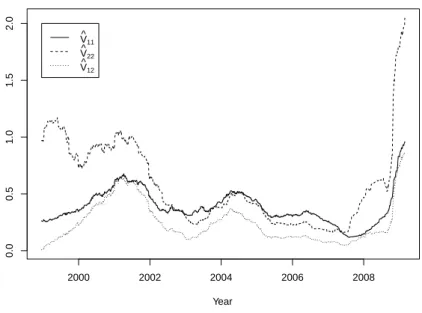
For the comparison purposes we plot the rolling estimator of the unconditional covariance matrix in Figure 2 given by
ˆ
V= 1
n−1
n
X
i=1
(X−X¯)(X−X¯)′.
The estimation window is set to be 250. In the figure, we observe that the estimator of the
covari-ance matrix is time varying. Significant increases in the elements of ˆVare present at the end of
2001 and during the financial crisis in 2008.
TheM E l AR(µ,Σ, 1)process is fitted to the considered data by using the two-stage maximum
likelihood estimator of Section 3. It holds thatα0=0.6944α1=0.6605 which are both
signif-icant at 1% level of significance. Using these values, we calculate the realizations of the
pseudo-generating variable ˆR2. The dispersion matrix ˆΣis estimated as in (16) by using the rolling
estima-tion with the estimaestima-tion window of 250 days. The results are presented in Figure 3. We observe that a large amount of the time variable behavior of the covariance matrix of the exchange rate returns is included in the pseudo-generating variable of the process. It increases significantly in the time periods, when the elements of the unconditional covariance matrix are larger. From the other side we get the considerable reduction of the time variability in the dispersion matrix, espe-cially, in the non-diagonal elements of the dispersion matrix which appears to be slowly varying with time.
5. SUMMARY
2000 2002 2004 2006 2008
0.0
0.5
1.0
1.5
2.0
Year V^11
V^22
V^12
Figure 2 –The rolling estimator for the unconditional covariance matrix with the estimation win-dow of 250 days.
1998 2000 2002 2004 2006 2008
0
5
10
15
20
25
30
Year
R
^t
2000 2002 2004 2006 2008
0.0
0.2
0.4
0.6
0.8
1.0
1.2
Year
Σ^ 11
Σ^22
Σ^ 12
Figure 3 –Estimators for the generating variable and the dispersion matrix of the daily EUR/USA
and EUR/JPY exchange rate returns for the period from January 2, 1999 to November 30, 2009.
elliptically contoured distributions. Moreover, the number of unknown parameters of the model is significantly reduced in comparison to other multivariate GARCH processes.
In the empirical study the daily EUR/USD and EUR/JAP exchange rate returns are used for
estimating the dispersion matrix of the MElAR process. The parameters of the process are esti-mated by the two-stage quasi maximum likelihood method. The obtained results do not support the volatile behavior of the dispersion matrix. The time variability of the covariance matrix is explained by the time varying behavior of the generating variable that influences the coefficient of the investor’s risk aversion (see, e.g. Bodnar and Gupta (2009a)).
The possible generalization of the obtained results can be done in two ways. First, heavy
tailed distributions, like the multivariatet-distribution, can be considered as a model for the
er-ror process. Second, the time varying dispersion matrix can be incorporated into the model. It could be done by using the exponential smoothing or to model the time varying dispersion matrix keeping the idea of the DCC process (see Engle (2002)).
ACKNOWLEDGEMENTS
The authors are thankful to the Referee and the Editor for their suggestions which have improved the presentation in the paper.
REFERENCES
J. BERK(1997).Necessary conditions for the capm. Journal of Economic Theory, 73, pp. 245–257.
R. BLATTBERG, N. GONEDES(1974). A comparison of the stable and student distributions as statistical models for stock prices. The Journal of Business, 47, pp. 244–280.
T. BODNAR, A. GUPTA(2009a). Construction and inferences of the efficient frontier in elliptical models. Journal of the Japan Statistical Society, 39, pp. 193–207.
T. BODNAR, A. GUPTA(2009b).An identity for multivariate elliptically contoured matrix distri-bution. Statistics and Probability Letters, 79, pp. 1327–1330.
T. BOLLERSLEV(1986).Generalized autoregressive conditional heteroscedasticity. Journal of
Econo-metrics, 31, pp. 307–327.
P. BOUGEROL, N. PICARD(1992). Stationarity of garch processes and of some nonnegative time series. Journal of Econometrics, 52, pp. 115–127.
G. CHAMBERLAIN(1983).A characterization of the distributions that imply mean-variance utility functions. Journal of Economic Theory, 29, pp. 185–201.
D. DEY, C. SRINIVASAN(1985). Estimation of covariance matrix under stein’s loss. Annals of
Statistics, 13, pp. 1581–1591.
R. ENGLE(2002). Dynamic conditional correlation – a simple class of multivariate garch models.
Journal of Business and Economic Statistics, 20, pp. 339–350.
R. ENGLE, K. SHEPPARD(2001).Theoretical and empirical properties of dynamic conditional
cor-relation multivariate garch. NBER Working Paper 8554.
E. FAMA(1965).The behavior of stock market price. Journal of Business, 38, pp. 34–105.
K. FANG, S. KOTZ, K. NG(1990). Symmetric Multivariate and Related Distributions. London: Chapman and Hall.
K. FANG, Y. ZHANG(1990). Generalized Multivariate Analysis. Berlin: Springer-Verlag and
Bei-jing: Science Press.
L. HAFF(1979a).An identity for the wishart distribution with applications. Journal of Multivariate
Analysis, 9, pp. 531–542.
L. HAFF(1979b). Estimation of the inverse convariance matrix: Random mixtures of the inverse
wishart matrix and the identity. Annals of Statistics, 7, pp. 1264–1276.
L. HAFF(1980).Empirical bayes estimation of the multivariate normal covariance matrix. Annals
of Statistics, 8, pp. 586–597.
L. HAFF(1991). The variational form of certain bayes estimators. Annals of Statistics, 19, pp.
1163–1190.
B. HANSEN(1994).Autoregressive conditional density estimation. International Economic Review, 35, pp. 705–730.
D. HODGSON, O. LINTON, K. VORKINK(2002).Testing the capital asset pricing model efficiency under elliptical symmetry: a semiparametric approach. Journal of Applied Econometrics, 17, pp. 617–639.
W. JAMES, C. STEIN(1961).Estimation with quadratic loss. InProc. Fourth Berkeley Symp. Math.
Statist. Prob. 1. Univ. California Press, Berkeley, pp. 361–380.
T. KUBOKAWA(2005). A revisit to estimation of the precision matrix of the wishart distribution. Journal of Statistical Research, 39, pp. 91–114.
T. KUBOKAWA, M. SRIVASTAVA(1999).Robust improvement in estimation of a covariance matrix in an elliptically contoured distribution. Annals of Statistics, 27, pp. 600–609.
W. NEWEY, D. MCFADDEN(1994).Large sample estimation and hypothesis testing. In R. ENGLE,
D. MCFADDEN(eds.),Handbook of Econometrics, vol 4, Elsevier Science, pp. 2111–2245.
J. OWEN, R. RABINOVITCH(1983).On the class of elliptical distributions and their applications to
the theory of portfolio choice. The Journal of Finance, 38, pp. 745–752.
M. PAWLAK, W. SCHMID(2001). On the distributional properties of garch processes. Journal of Time Series Analysis, 22, pp. 339–352.
M. ROCKINGER, E. JONDEAU(2002).Entropy densities with an application to autoregressive con-ditional skewness and kurtosis. Journal of Econometrics, 106, pp. 119–142.
G. SAMORODNITSKY, M. S. TAQQU(1994). Stable Non-Gaussian Random Processes, Stochastic Models with Infinite Variance. Chapman and Hall: New York, London.
C. STEIN(1956). Inadmissibility of the usual estimator for the mean of a multivariate normal
dis-tribution. InProc. Third Berkeley Symp. Math. Statist. Prob. 1. Univ. California Press, Berkeley, pp. 197–206.
G. ZHOU(1993). Asset-pricing tests under alternative distributions. The Journal of Finance, 48, pp. 1927–1942.
SUMMARY
Multivariate elliptically contoured autoregressive process
In this paper, we introduce a new class of elliptically contoured processes. The suggested process possesses both the generality of the conditional heteroscedastic autoregressive process and the elliptical symmetry of the elliptically contoured distributions. In the empirical study we find the link between the conditional time varying behavior of the covariance matrix of the returns and the time variability of the investor’s coefficient of risk aversion. Moreover, it is shown that the non-diagonal elements of the dispersion matrix are slowly varying in time.