A Color Image Quantization Algorithm Based on Particle Swarm Optimization

A Color Image Quantization Algorithm Based on Particle Swarm

Optimization

Mahamed G. Omran and Andries P. Engelbrecht Department of Computer Science

University of Pretoria

Pretoria 0002, SOUTH AFRICA

E-mail: [email protected], [email protected] Ayed Salman

Department of Computer Engineering Kuwait University

KUWAIT

Phone: +965-4811188-5833 Fax: +965-4817451 E-mail: [email protected]

Keywords: Color image quantization, K-means clustering algorithm, particle swarm optimization, post-clustering quantization approaches, pre-clustering quantization approaches

Received: February 6, 2005

A color image quantization algorithm based on Particle Swarm Optimization (PSO) is developed in this paper. PSO is a population-based optimization algorithm modeled after the simulation of social behavior of bird flocks and follows similar steps as evolutionary algorithms to find near-optimal solutions. The proposed algorithm randomly initializes each particle in the swarm to contain K centroids (i.e. color triplets). The K-means clustering algorithm is then applied to each particle at a user-specified probability to refine the chosen centroids. Each pixel is then assigned to the cluster with the closest centroid. The PSO is then applied to refine the centroids obtained from the K-means algorithm. The proposed algorithm is then applied to commonly used images. It is shown from the conducted experiments that the proposed algorithm generally results in a significant improvement of image quality compared to other well-known approaches. The influence of different values of the algorithm control parameters is studied. Furthermore, the performance of different versions of PSO is also investigated.

Povzetek: Evolucijski algoritem na osnovi jate ptičev je uporabljen za barvno obdelavo slik.

1

Introduction

Color image quantization is the process of reducing the number of colors presented in a digital color image [2]. Color image quantization can be formally defined as follows [27]:

Given a set of

N

_S′ colors where

_S

′

⊂

ℜ

Nd

and Nd is the dimension of the data space. The color quantization is a map

f

_q

:

S

′

→

S

′′

where

S

′′

is a set of

N

S′′ colors

such that

S

′′

⊂

S

′

and

N

_S′′

<

N

_S′. The objective is to minimize the quantization error resulting from replacing a color

c

∈

S

′

with its quantized value

f

_q

(

c

)

∈

S

′′

. Color image quantization is an important problem in the fields of image processing and computer graphics [27]:

• It can be used in lossy compression techniques [27];

• It is suitable for mobile and hand-held devices where memory is usually small [18]; • It is suitable for low-cost color display and

printing devices where only a small number of colors can be displayed or printed simultaneously [20].

• Most graphics hardware use color lookup tables with a limited number of colors [8]. Color image quantization consists of two major steps:

• Creating a colormap (or palette) where a small set of colors (typically 8-256 [20]) is chosen from the (224) possible combinations of red, green and blue (RGB).

• Mapping each color pixel in the color image to one of the colors in the colormap.

the global optimal solution because this will require a prohibitive amount of time. To address this problem, several approximation techniques have been used. One popular approximation method is the use of a standard local search strategy such as K-means. K-means has already been applied to the color image quantization problem [22], [3]. However, K-means is a greedy algorithm which depends on the initial conditions, which may cause the algorithm to converge to suboptimal solutions. This drawback is magnified by the fact that the distribution of local optima is expected to be broad in the color image quantization problem due to the three dimensional color space. In addition, this local optimality is expected to affect the visual image quality. The local optimality issue can be addressed by using stochastic optimization schemes.

In this paper, a new color image quantization algorithm based on Particle Swarm Optimization (PSO) is proposed. PSO is a population-based stochastic optimization algorithm modeled after the simulation of the social behavior of bird flocks and follows similar steps as evolutionary algorithms to find near-optimal solutions. PSO and other evolutionary algorithms that depend on heuristics to find 'soft' solutions are considered to be soft computing algorithms. This population-based search approach reduces the effect of the initial conditions, compared to K-means (especially if the size of the population is relatively large). The feasibility of the approach is demonstrated by applying it to commonly used images. The results show that, in general, the proposed approach performs better than

state-of-the-art color image quantization approaches. The rest of the paper is organized as follows. Section 2 surveys related work in the field of color image quantization. An overview of PSO is shown in section 3. The proposed algorithm is presented in section 4, while an experimental evaluation of the algorithm is provided in section 5. Finally, section 6 concludes the paper and provides guidelines for future research.

2

Related Work

Several heuristic techniques for color image quantization have been proposed in the literature. These techniques can be categorized into two main categories: pre-clustering and post-pre-clustering. The next subsections discuss each of these categories.

2.1

Pre-clustering approaches

Pre-clustering approaches divide the color into disjoint regions of similar colors. A representative color is then determined from each region. These representatives form the colormap. There are many fast algorithms in this category which are commonly used.

The median cut algorithm (MCA) [10] is often used in image applications because of its simplicity [8]. MCA divides the color space repeatedly along the median into rectangular boxes until the desired number of colors is obtained.

The variance-based algorithm (VBA) [28] also divides the color space into rectangular boxes. However, in VBA the box with the largest mean squared error between the colors in the box and their mean is split.

The octree quantization algorithm [9] repeatedly subdivides a cube into eight smaller cubes in a tree structure of degree eight. Then adjacent cubes with the least number of pixels are merged. This is repeated until the required number of colors is obtained [5]. Octree produces results similar to MCA, but with higher speed and smaller memory requirements [8].

Xiang and Joy [32] proposed an agglomerative clustering method which starts with each image color as a separate cluster. Small clusters are then repeatedly clustered into larger clusters in a hierarchical way until the required number of colors is obtained. The abandoning of the fixed hierarchical division of the color space is a significant improvement over the octree approach [32]. A similar approach called Color Image Quantization by

Pairwise Clustering was proposed by [27]. In this approach, a relatively large set of colors is chosen. An image histogram is then created. Two clusters that minimize the quantization error are then selected and merged together. This process is repeated until the required number of colors is obtained. According to [27], this approach performed better than MCA, VBA, octree, K-means and other popular quantization algorithms when applied to the two colored images used in their experiments.

Xiang [31] proposed a color image quantization algorithm that minimizes the maximum distance between color pixels in each cluster (i.e. the intra-cluster distance). The algorithm starts by assigning all the pixels into one cluster. A pixel is then randomly chosen as the

head of the cluster. A pixel that is the most distant from its cluster head is chosen as the head of a new cluster. Then, pixels nearer to the head of the new cluster move towards the new head forming the new cluster. This procedure is repeated until the desired number of clusters is obtained. The set of cluster heads forms the colormap. A hybrid competitive learning (HCL) approach combining competitive learning and splitting of the color space was proposed by [19]. HCL starts by randomly choosing a pixel as a cluster centroid. Competitive learning is then applied resulting in assigning all the image pixels to one cluster surrounding the centroid. A splitting process is then conducted by creating another copy of the centroid; competitive learning is then applied on both centroids. This process is repeated until the desired number of clusters is obtained. According to [19], HCL is fast, completely independent of initial conditions and can obtain near global optimal results. When applied to commonly used images, HCL outperformed MCA, VBA and K-means, and performed comparably with competitive learning [19], [20].

cluster along the axis H1, H2 or H3 of greatest variance. According to [2], the proposed approach generates images with comparable quality to that obtained from better but slower methods in this category.

Recently, Cheng and Yang [4] proposed a color image quantization algorithm based on color space dimensionality reduction. The algorithm repeatedly sub-divides the color histogram into smaller classes. The colors of each class are projected into a line. This line is defined by the mean color vector and the most distant color from the mean color. For each class, the vector generated from projection is then used to cluster the colors into two representative palette colors. This process is repeated until the desired number of representative colors is obtained. All color vectors in each class are then represented by their class mean. Finally, all these representative colors form the colormap. According to [4], this algorithm performed better than MCA, and performed comparably to SOM when applied on commonly used images.

2.2

Post-clustering approaches

The main disadvantage of the pre-clustering approaches is that they only work with color spaces of simple geometric characteristics. On the other hand, post-clustering approaches can work with arbitrary shaped clusters. Post-clustering approaches perform clustering of the color space [4]. A post-clustering algorithm starts with an initial colormap. It then iteratively modifies the colormap to improve the approximation. The major disadvantage of post-clustering algorithms is the fact that it is time consuming [8].

The K-means algorithm is one of the most popular post-clustering algorithms. It starts with an initial set of colors (i.e. initial colormap). Then, each color pixel is assigned to the closest color in the colormap. The colors in the colormap are then recomputed as the centroids of the resulting clusters. This process is repeated until convergence. The K-means algorithm has been proven to converge to a local optimum [8]. As previously mentioned, a major disadvantage of K-means is its dependency on initial conditions.

FCM [1] and Learning Vector Quantization [16] have also been used for color image quantization. Scheunders and De Backer [21] proposed a joint approach using both competitive learning and a dithering process to overcome the problem of contouring effects when using small colormaps.

Fiume and Quellette [7] proposed an approach which uses simulated annealing for color image segmentation. Pre-clustering approaches were used to initialize the colormap.

Self-Organizing Maps (SOMs) [15] were used by [5] to quantize color images. The approach selects an initial colormap, and then modifies the colors in the colormap by moving them in the direction of the image color pixels. However, to reduce the execution time, only samples of the colors in the image are used. According to [5], the algorithm performs better than MCA and octree.

Rui et al. [18] presented an initialization and training method for SOM that reduces the computational load of SOM and at the same time generates reasonably good results.

A hybrid approach combining evolutionary algorithms with K-means has been proposed by [8]. A population of individuals, each representing a colormap, are arbitrary initialized. Then, after each generation, the K-means algorithm (using a few iterations) is applied on each individual in the population. The standard error function of the Euclidean distance is chosen to be the fitness function of each individual. Based on the experiments conducted by [8], this hybrid approach outperformed both MCA and octree algorithms.

The Genetic C-means algorithm (GCMA) uses a similar idea where a hybrid approach combining a genetic algorithm with K-means was proposed by [20]. The fitness function of each individual in the population is set to be the mean square error (MSE), defined as

p K

k

k p

N

MSE

p k

∑ ∑

= ∀ ∈

=

1

2

)

(

C z

m

-z

(1)

As in [8], each chromosome represents a colormap. GCMA starts with a population of arbitrary initialized chromosomes. K-means is then applied to all the chromosomes to reduce the search space. A single-point crossover is then applied. This is followed by the application of mutation which randomly decides if a value of one is added to (or subtracted from) the gene's value (i.e. mutating the gene's value with ±1). All the chromosomes are then pairwise compared and the chromosome with the lowest MSE replaces the other chromosome. This process is repeated until a stopping criterion is satisfied. A faster version of this approach can be obtained by applying K-means to the best chromosome in each generation. For the remaining chromosomes, an approximation of K-means is used where a single iteration of K-means is applied on a randomly chosen subset of pixels. This process is repeated a user-specified number of times using different subsets. GCMA outperformed MCA, VBA, K-means, competitive learning and HCL when applied on commonly used images [19], [20]. However, GCMA is computationally expensive.

3

Particle Swarm Optimization

through the search space. Each particle represents a candidate solution to the optimization problem. The position of a particle is influenced by the best position visited by itself (i.e. its own experience) and the position of the best particle in its neighborhood (i.e. the experience of neighboring particles). When the neighborhood of a particle is the entire swarm, the best position in the neighborhood is referred to as the global best particle, and the resulting algorithm is referred to as the gbest PSO. When smaller neighborhoods are used, the algorithm is generally referred to as the lbest PSO [24]. The performance of each particle (i.e. how close the particle is to the global optimum) is measured using a fitness function that varies depending on the optimization problem.

Each particle in the swarm is represented by the following characteristics:

xi: The current position of the particle; vi: The current velocity of the particle; yi: The personal best position of the particle.

The personal best position of particle i is the best position (i.e. one resulting in the best fitness value) visited by particle i so far. Let f denote the objective function. Then the personal best of a particle at time step

t is updated as

⎩

⎨

⎧

<

+

+

≥

+

=

+

))

(

(

))

1

(

(

if

)

1

(

))

(

(

))

1

(

(

if

)

(

)

1

(

t

f

t

f

t

t

f

t

f

t

t

i i i i i i i

y

x

x

y

x

y

y

(2)

If the position of the global best particle is denoted by the vector

y

ˆ

, then

}

{

, , , min

{

( ()), ( ()), , ( ())

}

) (

ˆt y₀ y₁ ys f y₀ t f y₁t f ys t

y ∈ K = K (3)

where s denotes the size of the swarm. For the lbest model, a swarm is divided into overlapping neighborhoods of particles. For each neighborhood Nj, a best particle is determined with position

y

ˆ

_j. This particle is referred to as the neighborhood best particle, defined as

{

( ())

}

, } min )) 1 ( ˆ ( | { ) 1 (

ˆ_jt+ ∈N_j f y_j t+ = f y_i t ∀y_i∈N_j y

(4)

where

{

(

t

),

₁

(

t

),

,

₁

(

t

),

(

t

),

₁

(

t

),

,

₁

(

t

),

(

t

)

}

N

_j

=

y

_i−l

y

_i−l+

_K

y

_i−

y

_i

y

_i+

_K

y

_i+l−

y

_i+l

(5) Neighborhoods are usually determined using particle indices [25], however, topological neighborhoods can also be used [23]. It is clear that gbest is a special case of

lbest with l = s; that is, the neighborhood is the entire swarm. While the lbest approach results in a larger diversity, it is still slower than the gbest approach.

For each iteration of a PSO algorithm, the velocity vi update step is specified for each dimension j∈ 1,…, Nd, where Nd is the dimension of the problem. Hence, vi,j represents the jth element of the velocity vector of the ith particle. Thus the velocity of particle i is updated using the following equation:

)) ( ) ( )( ( )) ( ) ( )( ( ) ( 1)

(t wvt c₁r_1, t y t x t c₂r_2, t yˆ t x t

v_i,j + = _i,j + _{j i,j} −_i,j + _{j j} −_i,j (6)

where w is the inertia weight [23],

c

1 and

c

2 are the acceleration constants and

r

_1,j,

r

_2,j

~

U

(0,1)

. Eq. 6 consists of three components, namely

• The inertia weight term, w, which serves as a memory of previous velocities. The inertia weight controls the impact of the previous velocity: a large inertia weight favors exploration, while a small inertia weight favors exploitation [24].

• The cognitive component,

y

_i

(

t

)

−

x

_i, which represents the particle's own experience as to where the best solution is.

• The social component,

y

ˆ

(

t

)

−

x

_i

(

t

)

, which represents the belief of the entire swarm as to where the best solution is. Different social structures have been investigated [11], [14], with the star topology being used most. The position of particle i, xi, is then updated using the following equation:

)

1

(

)

(

)

1

(

t

+

=

_i

t

+

_i

t

+

i

x

v

x

(7)

The reader is referred to [26] and [17] for a study of the relationship between the inertia weight and acceleration constants, in order to select values which will ensure convergent behavior. Velocity updates can also be clamped through a user defined maximum velocity, Vmax, which would prevent them from exploding, thereby causing premature convergence [26].

The PSO algorithm performs the update equations above, repeatedly, until a specified number of iterations have been exceeded, or velocity updates are close to zero. The quality of particles is measured using a fitness function which reflects the optimality of a particular solution.

4

The PSO-based Color Image

Quantization (PSO-CIQ)

Algorithm

This section defines the terminology used throughout this paper. A measure is given to quantify the quality of the resultant quantized image, after which the PSO-CIQ algorithm is introduced.

• Np denotes the number of image pixels • K denotes the number of clusters (i.e.

colors in the colormap)

• zp denotes the coordinates of pixel p • mk denotes the centroid of cluster k

(representing one color triple in the colormap)

In this paper, the terms centroid and color triplet are used interchangeably.

4.1

Measure of Quality

The most general measure of performance is the mean square error (MSE) of the quantized image using a specific colormap. The MSE was defined in Eq. 1, and is repeated here for convenience:

p K

k

k p

N

MSE

p k

∑ ∑

= ∀ ∈

=

1

2

)

(

C z

m

-z

(8)

where Ck is the kth cluster.

4.2

The PSO-CIQ Algorithm

In this section, a new post-clustering color image quantization approach is described. The proposed approach is of the class of quantization techniques that performs clustering of the color space.

In the context of color image quantization, a single particle represents a colormap (i.e. a particle consists of K cluster centroids representing RGB color triplets). The RGB coordinates in each color triple are floating-point numbers. Each particle xi is constructed as xi = (mi,1,…,mi,k,…,

m

_i,K) where mi,k refers to the kth cluster centroid vector of the ith particle. Therefore, a swarm represents a number of candidate colormaps. The quality of each particle is measured using the MSE (defined in Eq. 8) as follows:

)

(

)

(

_i

MSE

_i

f

x

=

x

(9)

The algorithm initializes each particle randomly from the color image to contain K centroids (i.e. color triplets). The set of K color triplets represents the colormap. The K-means clustering algorithm is then applied to each particle at a user-specified probability, pkmeans. The K-means algorithm is used in order to refine the chosen colors and to reduce the search space. Each pixel is then assigned to the cluster with the closest centroid. The fitness function of each particle is calculated using Eq. 9. The PSO velocity and update Eq.'s 6 and 7 are then applied. The procedure is repeated until a stopping criterion is satisfied. The colormap of the global best particle after tmax iterations is chosen as the optimal result.

The PSO-CIQ algorithm is summarized below:

1. Initialize each particle by randomly choosing K color triplets from the image.

2. For t = 1 to tmax (a) For each particle i

i. Apply K-means for a few iterations with a probability pkmeans.

ii. For each pixel zp

Calculate

d

2

(

z

_p

−

m

_i,k

)

for all clusters

C

_i,k. Assign zpto

C

_i,kk where

{

(

)

}

)

(

2

1 2

k i, p K , , k kk i,

p

min

d

d

z

−

m

=

z

−

m

=

∀ K

iii. Calculate the fitness,

f

(

x

_i

)

(b) Find the global best solution

y

ˆ

(

t

)

(c) Update the centroids using Eq.'s 6 and 7

In general, the complexity of the PSO-CIQ algorithm is

O(sKtmaxNp). The parameters s, K and tmax can be fixed in advance. Typically s, K and tmax << Np. Therefore, the time complexity of PSO-CIQ is O(Np). Hence, in general the algorithm has linear time complexity in the size of a data set.

5

Experimental Results

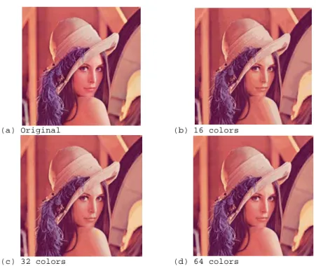
The PSO-CIQ algorithm was applied to a set of four commonly used color images namely: Lenna (shown in Figure 1(a)), peppers, jet and mandrill. The size of each image is 512 × 512 pixels. All images are quantized to 16, 32 and 64 colors.

The rest of this section is organized as follows: Section 5.1 illustrates that the PSO-CIQ can be used successfully as a color image quantization algorithm by comparing it to other well-known color image quantization approaches. Section 5.2 investigates the influence of the different PSO-CIQ control parameters. Finally, the use of different PSO models (namely, gbest, lbest and

lbest-to-gbest) are investigated in section 5.3.

colors, and a Kohonen network of 8×8 nodes was used when quantizing an image to 64 colors. All SOM parameters were set as in Pandya and Macy [17]: the learning rate

η

(

t

)

was initially set to 0.9 then decreased by 0.005 until it reached 0.005, the neighborhood function

∆

w

(

t

)

_{was initially set to (4+4)/4 for 16}

colors, (8+4)/4 for 32 colors, and (8+8)/4 for 64 colors. The neighborhood function is then decreased by 1 until it reached zero.

5.1

PSO-CIQ vs. Well-Known Color

Image Quantization Algorithms

This section presents results to compare the performance of the PSO-CIQ algorithm with that of SOM and GCMA for each of the test images.

Table 1 summarizes the results for the four images. The results of the GCMA represent the best case over several runs and are copied from [20]. The results are compared based on the MSE measure (defined in Eq. 8). The results showed that, in general, PSO-CIQ outperformed GCMA in all the test images except for the mandrill image and the case of quantizing the Jet image to 64 colors. Furthermore, PSO-CIQ generally performed better than SOM for both Lenna and peppers images. SOM and PSO-CIQ performed comparably when applied to the mandrill image. SOM generally performed better than PSO-CIQ when applied to the Jet image. Figure 1 show the visual quality of the quantized image generated by PSO-CIQ when applied to Lenna.

5.2

Influence of PSO-CIQ Parameters

The PSO-CIQ algorithm has a number of parameters that have an influence on the performance of the algorithm. These parameters include Vmax, the swarm size, the number of PSO iterations, pkmeans and the number of K-means iterations. This section investigates the influence of different values of these parameters using the Lenna image when quantized to 16 colors.

5.2.1 Velocity Clamping

Table 2 shows that using Vmax = 5 or Vmax = 255 generally produces comparable results.

5.2.2 Swarm Size

Increasing the swarm size from 20 to 50 particles slightly improves the performance of the PSO-CIQ algorithm as shown in Table 3. Similarly, increasing the swarm size from 50 to 100 particles slightly improves the performance of the PSO-CIQ algorithm. On the other hand, reducing the swarm size from 20 to 10 particles significantly reduces the efficiency of the PSO-CIQ algorithm. The rationale behind these results is that increasing the number of particles increases diversity, thereby limiting the effects of initial conditions and reducing the possibility of being trapped in local minima.

5.2.3 Number of PSO iterations

Increasing the number of PSO iterations, tmax, from 50 to 100 slightly improves the performance of the PSO-CIQ algorithm as shown in Table 4. Similarly, increasing tmax from 100 to 150 slightly improves the performance of the PSO-CIQ algorithm. Therefore, it can be concluded that increasing tmax generally improves the performance of the PSO-CIQ algorithm.

5.2.4 pkmeans

Applying the K-means clustering algorithm to a larger set of particles is expected to improve the performance of the PSO-CIQ algorithm. The rationale behind this expectation is the fact that the K-means algorithm generally reduces the search space and refines the chosen colors. This expectation is verified by the results shown in Table 5 which shows that increasing the value of

pkmeans generally improves the performance of the PSO-CIQ algorithm. However, as a trade-off, increasing the value of pkmeans will increase the computational requirements of the PSO-CIQ algorithm.

5.3

Number of K-means iterations

Reducing number of K-means iterations from 10 to 5 degrades the performance of the PSO-CIQ as shown in Table 6. On the other hand, increasing the number of K-means iterations from 10 to 50 significantly improves the performance of the PSO-CIQ as shown in Table 6. These results suggest that increasing the number of K-means iterations improves the performance of the PSO-CIQ. However, when the number of K-means iterations was reduced to 5 iterations but at the same time pkmeans was increased from 0.1 to 0.5 the generated MSE was equal to 210.315 ± 1.563 which is significantly better than the corresponding result in Table 6. This result suggests that the number of K-means iterations can be reduced without affecting the performance of PSO-CIQ given that the

pkmeans is increased.

5.4

Comparison of gbest-, and

lbest-to-gbest-PSO

In this section, the effect of different models of PSO is investigated using the Lenna image when quantized to 16 colors. A comparison is made between gbest-, lbest- and

lbest-to-gbest-PSO (which has been used in the above experiments) using a swarm size of 20 particles. For

lbest-PSO, a neighborhood size of l = 2 was used. Table 7 shows the result of the comparison. The results show no significant difference in performance.

6

Conclusion

performance of different versions of PSO was then investigated.

The PSO-CIQ uses the K-means clustering algorithm to refine the color triplets. Future research can investigate the use of other more efficient clustering algorithms such as FCM and KHM [33]. Finally, the PSO-CIQ uses the RGB color space. Although the RGB model is the most widely used model, it has some weaknesses. One of these weaknesses is that equal distances in the RGB color space may not correspond to equal distance in color perception. Hence, future research may try to apply the PSO-CIQ to other color spaces (e.g. the L*u*v* color space [29]).

References

[1] Balasubramanian R, Allebach J (1990) A new approach to platte selection for color images, Image

Technology 17: 284-290.

[2] Braquelaire J, Brun L (1997) Comparison and optimization of methods of color image quantization, IEEE Transactions on Image

Processing 6(7): 1048-1052.

[3] Celenk M (1990) A color clustering technique for image segmentation, computer vision, Graphics

and Image Processing 52: 145-170.

[4] Cheng S, Yang C (2001) A fast and novel technique for color quantization using reduction of color space dimensionality, Pattern Recognition Letters 22: 845-856.

[5] Dekker A (1994) Kohonen neural networks for optimal colour quantization, Network: Computation

in Neural Systems 5: 351-367.

[6] Engelbrecht A (2002) Computational Intelligence:

An Introduction, John Wiley and Sons.

[7] Fiume E, Quellette M (1989) On distributed, probabilistic algorithms for computer graphics,

Graphics Interface '89, 211-218.

[8] Freisleben B, Schrader A (1997) An evolutionary approach to color image quantization, Proceedings

of IEEE International Conference on Evolutionary Computation, 459-464.

[9] Gervautz M, Purgathofer W (1990) A Simple Method for Color Quantization: Octree Quantization, Graphics Gems, Academic Press, New York.

[10] Heckbert P (1982) Color image quantization for frame buffer display, ACM Computer Graphics 16(3): 297-307.

[11] Kennedy J (1999) Small worlds and mega-minds: effects of neighborhood topology on particle swarm performance, Proceedings of the Congress on

Evolutionary Computation, 1931-1938.

[12] Kennedy J, Eberhart R (1995) Particle swarm optimization, Proceedings of IEEE International

Conference on Neural Networks, Perth, Australia 4:1942-1948.

[13] Kennedy J, Eberhart R (2001) Swarm Intelligence, Morgan Kaufmann.

[14] Kennedy J, Mendes R (2002) Population structure and particle performance, Proceedings of the IEEE

Congress on Evolutionary Computation, Honolulu, Hawaii.

[15] Kohonen T (1989) Self-Organization and

Associative Memory, 3rd edn. Springer-Verlag, Berlin.

[16] Kotropoulos C, Augé E, Pitas I (1992) Two-layer learning vector quantizer for color image quantization, In: Vandewalle J, Boite R, Moonen M, Oosterlinck A (eds) Signal Processing IV:

Theories and Applications, 1177-1180.

[17] Pandya A, Macy R (1996) Pattern Recognition with

Neural Networks in C++, CRC Press.

[18] Rui X, Chang C, Srikanthan T (2002) On the initialization and training methods for Kohonen self-organizing feature maps in color image quantization, Proceedings of the First IEEE

International Workshop on Electronic Design, Test and Applications.

[19] Scheunders P (1997) A comparison of clustering algorithms applied to color image quantization,

Pattern Recognition Letters 18(11-13): 1379-1384. [20] Scheunders P (1997) A genetic C-means clustering

algorithm applied to color image quantization,

Pattern Recognition 30(6): 859-866.

[21] Scheunders P, De Backer S (1997) Joint quantization and error diffusion of color images using competitive learning, International

Conference on Image Processing 1:811.

[22] Shafer S, Kanade T (1987) Color Vision,

Encyclopedia of Artificial Intelligence, Wiley. [23] Shi Y, Eberhart R (1998) A modified particle

swarm optimizer, Proceedings of the IEEE

International Conference on Evolutionary Computation, Piscataway, NJ, 69-73.

[24] Shi Y, Eberhart R (1998) Parameter selection in particle swarm optimization, Proceedings of

Evolutionary Programming 98, 591-600.

[25] Suganthan P (1999) Particle swarm optimizer with neighborhood optimizer, Proceedings of the

Congress on Evolutionary Computation, 1958-1962.

[26] Van den Bergh F (2002) An analysis of particle

swarm optimizers, Ph.D. dissertation, Department of Computer Science, University of Pretoria. [27] Velho L, Gomes J, Sobreiro M (1997) Color image

quantization by pairwise clustering, Proceedings of

the 10th _{Brazilian Symposium on Computer}

Graphics and Image Processing, 203-207.

[28] Wan S, Prusinkiewicz P, Wong S (1990) Variance-based color image quantization for frame buffer display, Color Research and Application 15(1): 52-58.

[29] Watt A (1989) Three-Dimensional Computer

Graphics, Addison-Wesley.

[30] Wu X, Zhang K (1991) A better tree-structured vector quantizer, Proceedings IEEE Data

Compression Conference, 392-401.

[31] Xiang Z (1997) Color image quantization by minimizing the maximum inter-cluster distance,

[32] Xiang Z, Joy G (1994) Color image quantization by agglomerative clustering, IEEE Computer Graphics

and Applications 14(3): 44-48.

[33] Zhang B (2000) Generalized K-Harmonic means - boosting in unsupervised learning, Technical

Report HPL-2000-137, Hewlett-Packard Labs.

Tables:

Table 1. Comparison between SOM, GCMA and PSO-CIQ

Image K SOM GCMA PSO-CIQ

16 235.6 ± 0.490 332 210.203 ±

1.487

32 126.400 ±

1.200

179 119.167 ±

0.449 Lenna

64 74.700 ±

0.458

113 77.846 ±

16.132

16 425.600 ±

13.162

471 399.63 ±

2.636

32 244.500 ±

3.854

263 232.046 ±

2.295 Peppers

64 141.600 ±

0.917

148 137.322 ±

3.376

16 121.700 ±

0.458

199 122.867 ±

2.0837

32 65.000 ±

0.000

96 71.564 ±

6.089 Jet

64 38.100 ±

0.539

54 56.339 ±

11.15

16 629.000 ±

0.775

606 630.975 ±

2.059

32 373.600 ±

0.490

348 375.933 ±

3.42 Mandril

l

64 234.000 ±

0.000

213 237.331 ±

2.015

Table 2. Effect of Vmax on the performance of PSO-CIQ

using Lenna image (16 colors) MSE

Vmax=5 209.338 ± 0.402

Vmax=255 210.203 ± 1.487

Table 3. Effect of the swarm size on the performance of PSO-CIQ using Lenna image (16 colors)

MSE

s = 10 212.196 ± 2.458

s = 20 210.203 ± 1.487

s = 50 210.06 ± 1.11

s = 100 209.468 ± 0.703

Table 4. Effect of the number of PSO iterations on the performance of PSO-CIQ using Lenna image (16 colors)

MSE

tmax= 50 210.203 ± 1.487

tmax= 100 209.412 ± 0.531

Table 5. Effect of pkmeans on the performance of PSO-CIQ using Lenna image (16 colors)

MSE

pkmeans= 0.1 210.203 ± 1.487

pkmeans= 0.25 209.238 ± 0.74

pkmeans= 0.5 209.045 ± 0.594

pkmeans= 0.9 208.886 ± 0.207

Table 6. Effect of the number of K-means iterations on the performance of PSO-CIQ using Lenna image (16 colors) No. of K-means iterations MSE

5 212.627 ± 3.7

10 210.203 ± 1.487

50 208.791 ± 0.111

Table 7. Comparison of gbest-, lbest- and lbest-to-gbest- PSO versions of PSO-CIQ using Lenna image (16 colors)

MSE

gbest PSO 209.841 ± 0.951

lbest PSO 210.366 ± 1.846

lbest-to-gbest PSO 210.203 ± 1.487

Figures:

(a) Original (b) 16 colors

(c) 32 colors (d) 64 colors