Testing the limits of gradient sensing
Vinal Lakhani1,2, Timothy C. Elston1,3*
1 Curriculum in Bioinformatics and Computational Biology, University of North Carolina at Chapel Hill, Chapel
Hill, North Carolina, United States of America, 2 Battelle Center for Mathematical Medicine, Research Institute at Nationwide Children’s Hospital, Columbus, Ohio, United States of America, 3 Department of Pharmacology, University of North Carolina at Chapel Hill, Chapel Hill, North Carolina, United States of America
Abstract
The ability to detect a chemical gradient is fundamental to many cellular processes. In multi-cellular organisms gradient sensing plays an important role in many physiological processes such as wound healing and development. Unicellular organisms use gradient sensing to move (chemotaxis) or grow (chemotropism) towards a favorable environment. Some cells are capable of detecting extremely shallow gradients, even in the presence of significant molecular-level noise. For example, yeast have been reported to detect pheromone gradi-ents as shallow as 0.1 nM/μm. Noise reduction mechanisms, such as time-averaging and the internalization of pheromone molecules, have been proposed to explain how yeast cells filter fluctuations and detect shallow gradients. Here, we use a Particle-Based Reaction-Dif-fusion model of ligand-receptor dynamics to test the effectiveness of these mechanisms and to determine the limits of gradient sensing. In particular, we develop novel simulation methods for establishing chemical gradients that not only allow us to study gradient sensing under steady-state conditions, but also take into account transient effects as the gradient forms. Based on reported measurements of reaction rates, our results indicate neither time-averaging nor receptor endocytosis significantly improves the cell’s accuracy in detecting gradients over time scales associated with the initiation of polarized growth. Additionally, our results demonstrate the physical barrier of the cell membrane sharpens chemical gradi-ents across the cell. While our studies are motivated by the mating response of yeast, we believe our results and simulation methods will find applications in many different contexts.
Author summary
In order to survive, many organisms must not only be able to detect the presence of a chemical compound, but also in which direction that compound increases or decreases in concentration. For example, bacteria cells prefer to move towards areas with high sugar concentrations. The process by which cells determine the direction of a chemical gradient is called “Gradient Sensing”. Of particular interest is the gradient sensing capability of yeast cells. These cells have been observed detecting the direction of extremely shallow gradients, which produce only a 2% difference in the number of molecules across the cell. Because the molecular-level noise is much larger than this signal, it is unclear what
noise-a1111111111 a1111111111 a1111111111 a1111111111 a1111111111 OPEN ACCESS
Citation: Lakhani V, Elston TC (2017) Testing the limits of gradient sensing. PLoS Comput Biol 13 (2): e1005386. doi:10.1371/journal.pcbi.1005386
Editor: Qing Nie, University of California Irvine, UNITED STATES
Received: August 11, 2016
Accepted: January 27, 2017
Published: February 16, 2017
Copyright:©2017 Lakhani, Elston. This is an open access article distributed under the terms of the
Creative Commons Attribution License, which permits unrestricted use, distribution, and reproduction in any medium, provided the original author and source are credited.
Data Availability Statement: All relevant data are within the paper and its Supporting Information files.
Funding: This work was supported by National Institute of General Medical Scienceshttps://www. nigms.nih.gov/Pages/default.aspxGrants: GM103870, GM079271 and GM114136. The funders had no role in study design, data collection and analysis, decision to publish, or preparation of the manuscript.
reduction mechanism the cell employs to reduce the noise and detect the signal. We devel-oped a 3D computational simulation platform to calculate and study the exact positions of molecules during this process. Our platform utilizes High Performance Computing clus-ters and GPGPUs. We find that, of the two prevailing models in the literature, neither time-averaging nor receptor endocytosis sufficiently reduces molecular noise for yeast cells to reliably detect chemical gradients before they initiate polarized growth. This find-ing implies yeast must possess a mechanism for reorientfind-ing the direction of growth after cell polarization has occurred. We also find the cell membrane and similarly, any other physical barrier nearby the cell can improve the cell’s likelihood of detecting the gradient. Our simulation methods and results will be applicable in other areas of research.
Introduction
The ability to detect the direction of a chemical gradient is fundamental to many biological processes. To survive or carryout their proper function, individual cells must be able to undergo directed growth (chemotropism) or movement (chemotaxis) toward chemical signals, such as nutrients or hormones. An ideal system for studying gradient sensing is chemotropism during the mating response ofS.Cerevisiae(yeast). Yeast cells can exist as one of two haploid types:MATa orMATα.MATa cells seek a mating partner by sensing a gradient of the
phero-moneα-factor secreted byMATαcells (Fig 1A).
Gradient sensing strategies fall into two major categories: temporal and spatial. Temporal sensing mechanisms, in which an organism moving through its environment compares the
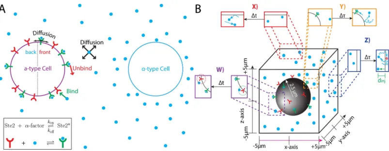
Fig 1. Computational platform for studying yeast gradient sensing. (A) MATαcells emit the mating pheromone ’α-factor’ (blue circle). Nearby MATa cells detect pheromone using the G-Protein Coupled Receptor Ste2 (red-shape = ’unbound’ state and green-shape with blue circle = ’bound’ state). Pheromone gradients must be detected in the presence of stochastic effects from pheromone binding (green arrow), unbinding (red arrow) and pheromone and receptor diffusion (black arrows). (B) Illustration of our Particle-Based Stochastic Reaction-Diffusion Model. During each time step (Δt), free receptors can capture pheromone molecules located within a specified capture radius (dashed green circle). Bound receptors randomly release a pheromone molecule a fixed distance (unbinding radius: dashed red circle) from the receptor. Pheromone molecules undergo 3D diffusion (each time stepΔt) and receptors diffuse on the cell surface (with a coarser time scaleΔτ). The ‘y’ and ‘z’ boundaries of the computational domain are reflective as well as the cell surface. Near the ‘x’ boundaries, pheromone molecules diffuse freely for a time (Δτ). AfterΔτtime, all pheromone molecules located outside the ‘x’ boundaries are removed. New pheromone molecules are injected everyΔτtime near the ‘x’ boundaries; each new molecule is placed a random distance (‘injection distance’) away from the ‘x’ boundary (green arrow, dinj).
concentration between its current and previous locations, are commonly utilized by small cells such asE.Coli(~1μm). Spatial sensing mechanisms, in which the organism compares the con-centration difference across the cell body, are commonly used by large cells including most eukaryotes, such asD.Discoideum(~15μm). The fact that yeast cells are not motile suggest they use a spatial sensing mechanism, despite being smaller (~4μm in diameter) than most eukaryotic cells.
Experimental studies have reported that yeast cells are capable of sensing linear gradients as shallow as 0.1 nM/μm [1,2]. All information on the extracellular pheromone gradient comes from receptors on the cell’s surface. Therefore, these receptors set the ultimate limits on gradi-ent sensing. To quantify the challenges faced by a cell in detecting shallow gradigradi-ents, we can estimate the average number of ligand-bound or active receptors (receptor occupancy) in the front half of the cell (pointing up the gradient) versus the back half of the cell (pointing down the gradient). We begin with estimating the size of the fluctuations about the mean receptor occupancy. The average receptor occupancy is roughly given byn¼N c
KDþc, where N is the
total number of receptors; KDis the dissociation constant, and c is the average concentration. The average occupancy in each half can be estimated using the average concentration in the front (or back) of the cell. This expression is an approximation because it does not correctly take into account the spatial dependence of the gradient across the cell. For a cell with 10000 receptors in a linear pheromone gradient of 0.1 nM/μm centered at the KD(about 7 nM) of the receptor, the difference in receptor occupancy isΔn = nfront−nback45. This calculation esti-mates a less than 1% difference in receptor occupancy between the front & back of the cell. Fol-lowing the work of Lauffenburger [3], the magnitude of the fluctuations in receptor occupancy issn¼
ffiffiffiffiffiffiffiffiffiffiffiffiffiffiffiffi
N KDc
ðKDþcÞ2
q
50. Hence for a gradient of 0.1 nM/μm, the signal is masked by the noise:
Δn45± 50, and a cell cannot predict the direction of the gradient based on an instantaneous measurement of receptor occupancy.
To explain how cells overcome these fluctuations, various noise-reduction mechanisms have been proposed: including time-averaging, gradient sharpening via extracellular degrada-tion of pheromone by the protease Bar1 [4,5] and removal of active receptors via endocytosis to avoid resampling [6,7]. The limits of these mechanisms have been estimated using mathe-matical models. Time-averaging requires sufficient time for the cell to sample multiple binding and unbinding events. In the yeast mating system, the KDof Ste2 binding toα-factor is known to be around 7nM [8–12]. Reported values for the unbinding rate are extremely slow: on the order of 10−4–10−3s-1[12,13]. These values imply a binding rate on the order of 104–105 (Ms)-1, which is many orders of magnitude slower than the diffusion limit of approximately 109(Ms)-1. With a dissociation rate of 0.0011 s-1[12], changes in receptor occupancy occur on the order of 10’s of minutes. Given that yeast cells begin chemotropic growth within 30 min-utes of exposure to pheromone, there seems to be insufficient time for the cell to accurately sense a shallow gradient using the time-averaging mechanism alone.MATa cells secrete Bar1:
The results discussed above are based on mathematical models in which simplifying assumptions are made to allow analytic tractability. To go beyond these models, we built a simulation platform based on fundamental biophysical processes that allows us to evaluate noise-reduction mechanisms and study gradient sensing with minimal assumptions. In partic-ular, we develop a Particle-Based Stochastic Reaction-Diffusion Model to study receptor dynamics in a gradient (Fig 1B). We choose this approach, because non-particle-based meth-ods using Reaction Diffusion Master Equations (RDME), although computationally fast, dis-cretize space. This discretization implicitly assumes each computational voxel is well-mixed, which reduces spatial accuracy [16]. Additionally, these methods are difficult to implement when the computational domain has complex boundary conditions such as the partially absorbing boundaries we use to create a gradient. Currently available particle-based simulation packages, such as Smoldyn or MCell, treat 2ndorder reactions by assuming that once two reac-tants are within a specified capture radius, the reactions occurs with certainty [4,17]. However, for our system, the slow association rate would make the capture radius unphysically small. Thus, we choose to create our own Particle-Based Stochastic Reaction-Diffusion Model and use the methods developed by Erban and co-workers [18] to treat 2ndorder reactions. Their method allows for customization of the binding radius. We also develop novel methods for simulating the development of chemical gradients that do not exist in current publically avail-able software packages.
Our simulations reveal: 1) time-averaging and receptor cycling, wherein Ste2 exocytosis is isotropic (unpolarized), are insufficient for yeast cells to confidently detect the direction of shallow gradients before initiating polarized growth, and 2) isotropic exocytosis of Bar1 may improve gradient sensing for cells with fast reaction rates. Additionally, our simulations reveal that 1) the physical barrier of the cell membrane sharpens the gradient, and 2) diffusion of the receptor reduces the cell’s ability to detect the direction of the gradient. Our approach bridges the theoretical mathematical models andin vivoexperimental approaches.
Results
We are motivated by the ability of yeast cells to sense shallow pheromone gradients even in the presence of significant amounts of molecular noise. Accordingly, we set the biophysical parameter values in our simulations to match the yeast mating response system (Table 1). Although the KDof the Ste2 receptor is known to be around 7nM [8–12], there is no consensus for the binding and unbinding rates. The diffusion limit for binding is on the order of 109 (Ms)-1. However, one experimental study reported rates as slow as kon= 1.6×10⁵(Ms)-1and koff= 0.0011 s-1[12], and similar values were measured in [8]. Elsewhere, a computational model used rates ten times faster than these values; although, the experimental sources for these rates are unclear [11]. To compare how these rates affect gradient sensing, we consider both sets of reaction rates.
Section I: Equilibrium fluctuations in uniform pheromone concentration
Equilibrium fluctuations in receptor occupancy. Since the seminal work of Berg &
Pur-cell [19], there have been many theoretical studies on the limits with which Pur-cells can measure external ligand concentrations [6,20–23] and strategies for overcoming these limitations [6]. The two main sources of fluctuations considered by these studies are fluctuations in the ligand concentration and stochastic binding and unbinding of the ligand from the receptor. Our sim-ulations accurately capture these sources of noise as well as fluctuations from receptor diffu-sion. Our model also allows us to investigate non-equilibrium conditions and the effect of the cell in perturbing the ligand concentration profile. We show our simulation results agree most closely with the theory of Berezhkovskii and Szabo [20].
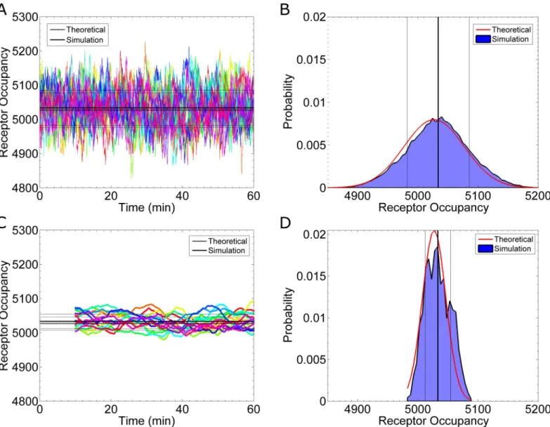
Most models assume the cell’s receptors are at equilibrium with an external, uniform ligand concentration. Therefore, we begin by performing simulations under equilibrium conditions. First, we initialize the system to have the expected number of active receptors and ligand mole-cules in the computational domain. Second, we allow the system to equilibrate for 30-minutes to generate a random state. Lastly, this random state is used as the initial condition for a 60-minute simulation, which we then analyze.Fig 2shows the results of sixteen simulations using the pa-rameters listed inTable 1, with the exceptions that: 1) there is no ligand gradient (g= 0 nM/μm) and 2) the reaction rates are taken to be kon= 1.6×10⁶(Ms)-1and koff= 0.011 s-1.Fig 2Ashows the receptor occupancy time series, n(t), andFig 2Bshows a histogram of the data.
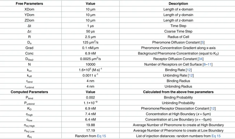
Table 1. Standard Parameter Set.
Free Parameters Value Description
XDom 10μm Length of x-domain
YDom 10μm Length of y-domain
ZDom 10μm Length of z-domain
Δt 1μs Time Step
Δτ 50μs Coarse Time Step
R 2.5μm Radius of Cell
Dα 125μm2/s Pheromone Diffusion Constant [5]
Grad 0.1 nM/μm Pheromone Concentration Gradient along x-axis
Conc 6.9 nM Background Pheromone Concentration (equal to KD)
DSte2 0.0025μm2/s Receptor Diffusion Constant [34]
N 10000 Number of Receptors on Cell Surface [8–11]
kon 1.6×10⁵(Ms)-1 Binding Rate [12]
koff 0.0011 s-1 Unbinding Rate [12]
rbind 4 nm Binding Radius
runbind 4 nm Unbinding Radius
Computed Parameters Value Calculated from the above free parameters
Pbind 0.002 Binding Probability
Punbind 1.1×10⁻⁹ Unbinding Probability
KD 6.9 nM Pheromone/Receptor Dissociation Constant [12]
chigh 7.4 nM Concentration at High Boundary (x = 5μm)
clow 6.4 nM Concentration at Low Boundary (x = –5μm)
ninj High 19.88 Average Number of Pheromone to create at High Boundary
ninj Low 17.19 Average Number of Pheromone to create at Low Boundary
dinj Random fromEq 15 List of injection distances: random numbers fromEq 15 The first set of values contains all the parameters necessary to uniquely define a stochastic simulation. The second set contains additional values that are calculated from the first set of parameters.
For uniform pheromone concentration, the mean and standard deviation can be calculated from the following equations:
n¼N c KDþc
ð1aÞ
sn¼
ffiffiffiffiffiffiffiffiffiffiffiffiffiffiffiffiffiffiffiffiffiffiffi
N KDc
ðKDþcÞ
2
s
ð1bÞ
Fig 2. Receptor Occupancy at Equilibrium. (A) Simulation results for the number of active receptors as a function of time. Each color represents a
different realization of the process. The thick, solid, black line is the mean from the data (5035 Ste2*). The thin, solid, black lines represent one standard deviation away from the mean, as calculated from the data (±52 Ste2*). The thick, dashed, black line is the theoretical mean calculated fromEq 1a(5027 Ste2*). The thin, dashed, black lines are one theoretical standard deviation from the mean as calculated fromEq 1b(±50 Ste2*). (B) A histogram of the data in (A). The vertical lines are equivalent to those in (A). The red curve shows the theoretical distribution. (C) A plot of time-averaged receptor occupancy. Each time point displays the average occupancy of the preceding 10 minutes. No average is available for t<10min. The black lines are similar to those in
(A). The simulation mean is 5034±23 Ste2*, and the theoretical mean is 5027±19 Ste2*. The theoretical mean is again calculated withEq 1a, but the time-averaged standard deviation is calculated fromEq 5and the relation described in the text. (D) A histogram of the data in (C). The time-averaged distribution is much narrower (σ= 23 Ste2*) than the instantaneous distribution (σ= 52 Ste2*). The parameters used for these simulations are reported inTable 1, with binding and unbinding rates of 1.6×10⁶(Ms)-1and 0.011 s-1, respectively, and no ligand gradient.
(derived in [3]). In both equations,Nis the total number of receptors; KDis the dissociation constant, andcis the concentration. InEq 1a,nis the average receptor occupancy, and inEq 1b,σn2is the variance of the receptor occupancy. Our simulations match the mean and stan-dard deviation of the receptor occupancy with the theoretical values (Fig 2A and 2B).
Time averaging. A common noise reduction technique from signal-processing is
time-averaging. Assume the receptor occupancy is averaged for a length of time,T, then starting with the instantaneous occupancy n(t) (Fig 2A), we calculate the time average asnTð Þ ¼t
1
T
PT=Dt
i¼1 nðt TþDtiÞ, whereΔt is sampling interval.Fig 2Cshows the time-averaged
occupancy for T = 10min. The resulting time-averaged standard deviation, which we label as sn
T, is 23 Ste2
molecules (Fig 2C and 2D). This time-averaged uncertainty is much smaller
than the instantaneous uncertainty, which is 52 Ste2molecules (Fig 2A and 2B).Fig 2D
shows the corresponding time-averaged histogram. The theoretical time-averaged values (dashed lines inFig 2Cand red curve inFig 2D) are calculated from the theoretical work of Berezhkovskii and Szabo [20]. Below, we discuss how these results compare with the other the-oretical models that have appeared in the literature.
In 1977, Berg & Purcell derive an expression for the lower bound on the accuracy a cell can achieve when time-averaging [19]:
CV2
¼sc
2
c2 ¼
1
pDRcT 1þ konc
koff
ð2Þ
wheresc2
c2 is the time-averaged variance in the concentration estimation divided by the average
concentration squared. Because this ratio is the Coefficient of Variation squared, we label it CV2. InEq 2,Dis the diffusion constant for the ligand;Ris the radius of the cell;cis the concentration of ligand, andTis the length of time-averaging. The Berg & Purcell model assumes the binding rate is diffusion-limited and the cell has an excessive number of receptors (NDR
kon) [19]. Hence, their conclusion shows the cell’s accuracy is limited by the stochastic arrival of ligand molecules to the cell [19]. In 2005, Bialek & Setayeshgar derived the CV2for a binding rate slower than the diffusion-limit [21]:
CV2
¼sc
2
c2 ¼
2 koncT
1þkonc
koff
þ 1
pDRcT ð3Þ
Eqs2&3were reconciled in 2014 by Kaizu et. al. [22]:
CV2
¼sc
2
c2 ¼
2 koncT
1þkonc
koff
þ 1
2pDRcT 1þ konc
koff
ð4Þ
The second term in Eqs3&4is the contribution from fluctuations in the arrival of ligand mol-ecules, similar toEq 2. The first term in Eqs3&4is the contribution from stochastic binding and unbinding reactions. Eqs3&4were derived for a single receptor in solution [24]. In 2013, Berezhkovskii & Szabo derived an expression for the CV2that includes both major sources of noise and considers an arbitrary number of receptors [20]:
CV2
¼sc
2
c2 ¼
2 NkoncT
1þkonc
koff
þ 1
2pDRcT 1þ konc
Nkoff
ð5Þ
varying lengths (T = {10, 20. . .3600} sec). For each value ofT, we compute the time average for each simulation (e.g. the case of T = 10min is shown inFig 2C) and then use these results to calculate the time-averaged variance:sn
T
2. We also can calculate the instantaneous variance
in receptor occupancy,σn2from the data presented inFig 2A. Therefore, as described in [20],
we calculate an empirical CV2using the relationship:CV2
¼snT2
sn4.
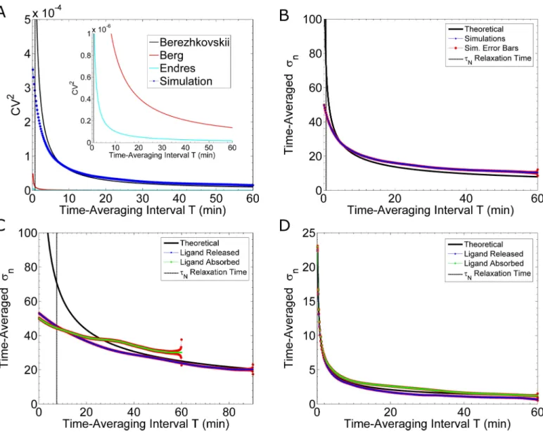
InFig 3Awe compare the theoretical results of the Berg & Purcell model [19] (red curve, Eq 2), the Berezhkovskii & Szabo model [20] (black curve,Eq 5) and our simulation results
Fig 3. Noise Reduction by Time-Averaging. (A) Comparison of theoretical and simulation results. The black curve is a plot ofEq 5, taken from Berezhkovskii & Szabo [20]; the black, dashed, vertical line is the relaxation time,τN. The theory is valid for T>>τN[20]. The red curve is a plot ofEq 2, taken from Berg & Purcell [19]. The teal curve is a plot ofEq 6, taken from Endres & Wingreen [6]. The blue curve is calculated from the simulations shown inFig 2A. Inset: Zoom in along the y-axis. (B) As in (A), the blue curve, with red standard error bars, is the result of simulations with fast reaction rates: 1.6×10⁶(Ms)-1and 0.011 s-1. The theoretical curve is fromEq 5. (C) Comparison of Ligand Releasing and Ligand Absorbing models. These simulations use the measured (see [12]) binding rate of kon= 1.6×10⁵(Ms)-1and either an unbinding rate of koff= 0.0011 s-1(blue curve) or an endocytosis rate of kEndo= 0.0011 s-1(green curve). The blue curve is calculated from twenty-six simulations, and the green curve is calculated from eight simulations. The standard error for each calculation is shown in red. (D) Comparing the Ligand Releasing and Ligand Absorbing models. These simulations use rates 500 times faster than those in (C). That is, the binding rate is kon= 8×10⁷(Ms)-1; the unbinding rate is koff= 0.55 s-1(blue curve); while, the endocytosis rate is kEndo= 0.55 s-1(green curve). We calculate the blue and green curves from ten simulations each. The standard error for each calculation is shown in red.
(dotted, blue curve). As discussed above,Eq 2is derived from a model which predicts the cell’s accuracy is solely limited by the stochastic arrival of pheromone molecules [19].Eq 5is derived from a model which predicts the cell’s accuracy is additionally limited by the stochasticity of binding and unbinding reactions [20]. Our simulated data agree well with the results of Berezhkovskii & Szabo (Fig 3A), demonstrating that the stochastic binding and unbinding events contribute significantly to fluctuations in receptor occupancy.
A more intuitive representation of uncertainty is to plot the time-averaged standard devia-tion,sn
T, as a function of the length of time-averaging,T. We show that our simulations (blue
curves,Fig 3B–3D) agree with the theoretical predictions from Berezhkovskii and Szabo [20] (black curves,Fig 3B–3D). In addition, results from our simulations are complementary to the theoretical model, in that, our simulations can estimate the uncertainty of short time-averaging lengths, for which the theory fails. Specifically, the theoretical model is valid only for T>>τN, where,τNis the equilibration time scale of the system or ‘relaxation time’ [20]. In the case of slow reaction rates (kon= 1.6×10⁵(Ms)-1and koff= 0.0011 s-1),τN7.5min, which is roughly the inverse of the sum of the rates. The theoretical predictions diverge from our simulation results for T<40min (blue curve,Fig 3C). This time scale is comparable to the time at which yeast cells exposed to pheromone initiate polarized growth (~ 30 minutes after pheromone exposure). Hence our simulated results estimate the time-averaged uncertainty for biologically relevant time-scales, which current theories do not capture. InFig 3B–3D, we compare the ef-fectiveness of time-averaging between the two different sets of reaction rates discussed above. For fast rates, as used in [11], there is significant noise-reduction when time-averaging for short lengths of time: 10min or less (Fig 3B). Whereas, for slow rates, as measured in [12], time-averaging for as long as 20min only nominally reduces the noise (blue curve,Fig 3C). Thus, accurate measurements of the reaction rates are critical for determining how effectively time averaging can reduce noise.
The “perfectly absorbing” cell and receptor cycling. In addition to time-averaging,
End-res & Wingreen propose that a cell which “perfectly absorbs” ligand molecules, can more accu-rately measures an external ligand concentration [6]. A “perfect absorber” is a cell which, after binding a ligand molecule, does not release that ligand molecule back into the environment. Therefore, Endres & Wingreen argue, the cell does not count the same ligand molecule more than once. Similar to Berg & Purcell’s work [19], this model assumes that the binding rate is diffusion-limited and that there are an infinite number of receptors. Endres & Wingreen derive the following expression for the cell’s accuracy under this mechanism [6]:
CV2
¼sc
2
c2 ¼
1
4pDRcT ð6Þ
We find this model does not match our simulation results (Fig 3A). We can analytically compare this model to the Berezhkovskii & Szabo model [20], which best matches our si-mulation data.Eq 5is a more general expression for the CV2and reduces to a form similar toEq 6under certain limiting conditions. IfN c
KD, then the second term inEq 5simplifies:
1 2pDRcT 1þ
konc N kof f
1
2pDRcT. IfkoncNð1 nÞ ¼koncN= 1þ
konc kof f
4pDRc, wherenis the expected fractional occupancy, then the first term inEq 5is much smaller than the second term, and the expression reduces to the following expression:
CV2
¼sc
2
c2
1
2pDRcT ð7Þ
The two conditions used to derive the above expression, are closely related to the assumptions made for Eqs2&6. The first condition,N c
typical parameter sets, this condition is easily met. The second condition indicates that every ligand molecule which encounters the cell must be captured by an unbound receptor. This condition can be met by having a high reaction rate (kon), a large number of receptors (N), or both. Hence, if there are enough receptors and the binding rate is fast enough to guarantee the capture of every ligand molecule, then the cell’s accuracy is given byEq 7[20] (see also “The Perfect Instrument” in [19]).
The parameters in our simulations of the yeast system fail to meet these conditions and can-not be considered a “perfect absorber”. The binding rate is 3–4 orders of magnitude too slow. Nonetheless, we can simulate a partial absorber to determine if removing ligand from the envi-ronment, rather than releasing the ligand back into the envienvi-ronment, can improve the cell’s accuracy. A partial absorber does not absorb every ligand molecule that arrives at the surface. Endres & Wingreen suggest receptor cycling is a potential biological mechanism which enables the cell to absorb ligand [6]. Thus, we modify our simulation algorithm to include a simplified receptor cycling mechanism. In particular, we make the following changes to our algorithm (seeMethods: “Receptor Cycling Model”). An active receptor, Ste2, has some rate of endocy-tosis. Immediately upon endocytosis, an unbound receptor is created in a random position on the cell surface. Thus, in our simplified model, endocytosis is coupled with immediate replace-ment, which allows us to keep the total number of receptors constant. We also assume, Ste2 cannot unbind a ligand (koff= 0 s-1). We find that absorbing ligand molecules does not reduce the fluctuations in time-averaged receptor occupancy as compared to unbinding and releasing ligand molecules (Fig 3C and 3D).
Section II: At equilibrium in pheromone gradient
Gradient sharpening due to steric effects. To establish a linear pheromone gradient in
our simulations, we fix the pheromone concentration at the boundaries located at x = 5μm and x = –5μm (seeMethods: “Gradient Method 1”). For example, to create a 0.5 nM/μm gradi-ent with a concgradi-entration of 6.9nM at the midpoint, the concgradi-entration at x = –5μm is set to 4.4nM, and the concentration at x = 5μm is set to 9.4nM. In addition to these two boundaries, we set the boundary of the cell to be reflective, because the cell membrane is impermeable to pheromone. This impermeable boundary produces non-linear effects on the pheromone gra-dient, which we verify by calculating the concentration distribution within the computational space. For the calculation, we discretize the simulation space and count the average number of molecules in each bin. The molecules are tallied based on their x-position and distance from the x-axis (r¼pffiffiffiffiffiffiffiffiffiffiffiffiffiffiy2þz2). Additional details on this calculation are provided in the
Supple-mental Methods (S1 Text, Section E).Fig 4Ashows the average pheromone concentration profile for simulations (including reactions) with an impermeable cell membrane. This effect is not due to boundary conditions, because a similar profile is observed in simulations using larger volumes: (15μm)3(S2 Text, Section A). To confirm that the non-linear effects are solely
due to the physical boundary (and not due to the biochemical reactions), we repeat the simula-tions but allow pheromone molecules to freely diffuse through the membrane.Fig 4Bshows a profile for simulations (including reactions) with a permeable cell membrane. Without the dif-fusive barrier of the cell membrane, the concentration profile is linear (Fig 4B). Thus, we find the impermeability of the cell membrane produces nonlinear steric effects on the pheromone gradient, such that, the resulting gradient is steeper than expected (Fig 4A and 4B).
This sharpening effect is solely due to the impermeability of the cell membrane to phero-mone. Simulations in which pheromone are free to diffuse through the cell membrane, pro-duce a linear gradient:g¼@c
@x(Fig 4B). However, for an impermeable membrane, there is no flux across the cell boundary. Therefore, according to Fick’s Law,J¼ D@c
@n^¼0or @c
where^nis the vector normal to the cell surface. As predicted by this argument, the measured gradient@c
@xnear the boundary is close to 0 (Fig 4A). This constraint produces a higher than expected concentration at the front of the cell and a lower than expected concentration at the back of the cell. We next investigate whether this sharper gradient produces an appreciable dif-ference in the distribution of active receptors.
We first consider the fast set of reaction rates: kon= 1.6×10⁶(Ms)-1and koff= 0.011 s-1. As an initial approach to measuring the distribution of Ste2, we evaluate the receptor occupancy in the “front half” (x>0μm) and the “back half” (x<0μm). Assuming a true linear gradient, c
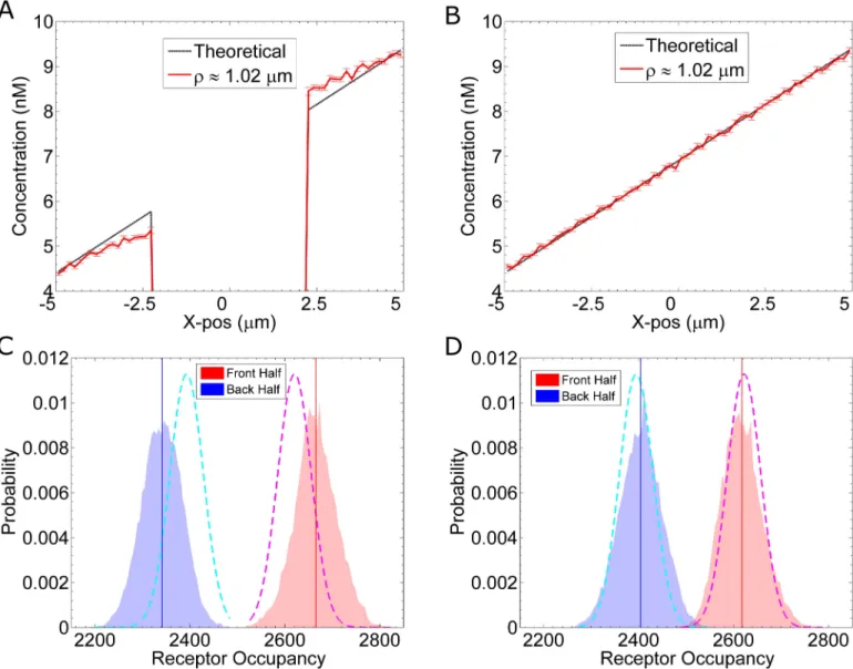
Fig 4. Gradient Sharpening Due to Steric Effects. We plot the pheromone concentration as a function of x, withr¼pffiffiffiffiffiffiffiffiffiffiffiffiffiffiy2þz21:02mm. The red
curve is calculated from our simulations, which include binding and unbinding reactions. The dashed, black line is the ideal, linear concentration profile.
(A) Results from eight simulations in which pheromone molecules reflect off the cell surface. There is no pheromone in the cell interior (x = –2.28μm to x = 2.28μm). (B) Same as (A), except that the reflecting cell boundary has been removed. That is, pheromone molecules can diffuse through the cell membrane, but are still able to bind receptors. (C) Histograms from the simulation results shown in (A). The blue and red histograms show the distributions for the number of active receptors, Ste2*, located in the back and front half of the cell, respectively. The solid vertical lines indicate the mean for their respective distributions. The dashed curves indicate the theoretical distribution for a cell in a linear gradient. (D) Same as (C) using data from simulations in (B), that is, with a permeable cell membrane.
(x) = gx + c0, we can calculate the mean and standard deviation of receptor occupancy using:
n¼N 1 b a
Z b
a
cðxÞ
KDþcðxÞ
dx ð8aÞ
sn2
¼N 1
b a
Z b
a
KDcðxÞ
ðKDþcðxÞÞ
2 dx ð8bÞ
which are more generalized forms ofEq 1. For example, in the front half, a = 0 and b = R,
which gives the following expression for the mean occupancy:nf ront¼NþNKD
gRln KDþc0
KDþc0þgR
. UsingEq 8, we estimate that in a true linear gradient, the number of active receptors in the back half is nback= 2395± 35 Ste2, and the number of active receptors in the front half is nfront= 2622± 35 Ste2(dashed lines,Fig 4C and 4D). From the simulation data, we count the number of occupied receptors located in each half at a given time. From simulations with an impermeable membrane, we calculate nback= 2341± 42 Ste2and nfront= 2665± 44 Ste2(Fig
4C). From simulations, in which pheromone are allowed to pass through the cell membrane unimpeded, we calculate nback= 2404± 45 Ste2and nfront= 2617± 43 Ste2(Fig 4D). Thus, we find steric effects from the cell membrane can locally sharpen the pheromone gradient. In turn, this sharpening can significantly improve the asymmetry in the distribution of active re-ceptors (Fig 4C and 4D). For a 0.5 nM/μm gradient, the difference in active receptors between the front and back (Δn = nfront−nback) changes fromΔn = 212 Ste2without sharpening to
Δn = 324 Ste2with sharpening, a more than 40% improvement.
Slow reaction rates and receptor diffusion add spatial noise. As shown inFig 4, the sharpened gradient increases the difference in receptor occupancy between the front and back for a system with fast reaction rates. To evaluate the sensitivity of the system with respect to the reaction rates, we repeat the simulations using the slow set of reaction rates: kon= 1.6×10⁵ (Ms)-1and koff= 0.0011 s-1. We find that, although the pheromone gradient is equivalently sharpened (S2 Text, Section B), the simulations with slow reaction rates do not show a larger
than expected difference in receptor occupancy between the front and back (Fig 5). Simula-tions with slow kinetics have a smaller difference in receptor occupancy,Δn = 238 Ste2(Fig
5A), than simulations with fast kinetics:Δn = 324 Ste2(Fig 4C). The cause for this discrep-ancy is receptor diffusion. A system with slow kinetics can increase the difference in receptor occupancy by reducing the receptor diffusion constant. For example, simulations with slow kinetics and no Ste2 diffusion (DSte2= 0μm
2
/s) (Fig 5B) show a larger difference in receptor occupancy,Δn = 315 Ste2, than simulations with receptor diffusion (Fig 5A).
One interpretation is that, a system with a slow unbinding rate allows activated receptors to diffuse long distances before reverting to the inactive state. For example, with a slow
un-binding rate of koff= 0.0011 s-1, a Ste2molecule typically diffuses
ffiffiffiffiffiffiffiffiffiffiffiffiffiffiffiffiffiffiffiffiffiffi
2DSte2 1
kof f
r
¼2:2mm, or
2:2mm
2:5mm
180
p 51
, away from the position at which it bound a pheromone molecule. Hence, many Ste2molecules will diffuse from the front half to the back half of the cell or vice-versa.
Because there are more Ste2in the front half than back half, there is a net flux of Ste2from
constant otherwise [25]. This two-state model is sufficient for creating a pom1p gradient on the cell membrane [25]
Time-averaging the estimated gradient direction. Up to this point, we have limited our
discussion to cells in a gradient of 0.5 nM/μm. Figs4Cand5Ashow that for this case, there is a clear difference in receptor occupancy in the front and back halves of the cell. However, for a shallow gradient, 0.1 nM/μm, there is significant overlap in the occupancy distributions for the two halves (S2 Text, Section C). Additionally, we have limited our analysis of the Ste2 distri-bution by dividing the cell into two halves. This division artificially introduces spatial informa-tion, because there are only two options for the direction of the gradient. In reality, the cell has no such spatial information; the full 2-dimensional distribution of active receptors must be considered to determine the direction of the gradient. As a measure of the cell’s estimate for the direction of the gradient, we use the direction of the vector that points from the origin (center of the cell) to the center of mass of the distribution of active receptors. We denote this vector asgest. InFig 6A and 6D, we present a phase plane of the azimuthal angle and elevation
(polar angle) ofgest. The elevation measures the angle ofgestrelative to the x-y plane. The
azi-muthal angle is the counterclockwise angle ofgestin the y plane away from the positive
x-axis.gestcoincides with the true direction of the gradient (^x) at the point (0, 0). InFig 6A, we
plot a trajectory ofgestfor a single cell.Fig 6Dshows the time-averaged trajectories of all sixteen
cells for an averaging window of 10 min. The remaining panels inFig 6report the angle between gestand the true direction of the gradient (^x), which we call “angular deviation”. An angular
deviation of 0 indicatesgestis aligned with the gradient and a value of 180 indicatesgestis pointed
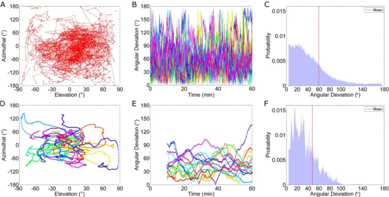
in the ^xdirection. InFig 6B, we plot the angular deviation for all 16 cells at each time point. We also plot the distribution of the angular deviation (Fig 6C).Fig 6Eshows trajectories for the time-averaged angular deviations and the corresponding distribution is shown inFig 6F. By comparing the distributions (Fig 6C and 6F), we find time-averaging improves the likelihood that the average position, or center of mass, of Ste2correctly points towards the gradient.
From the distributions, we can calculate the probability that the cell’s estimate of the gradi-ent is accurate within a given threshold. For example, from the instantaneous distribution (Fig
Fig 5. Receptor Diffusion adds Spatial Noise. These curves are similar to those inFig 4except with slow reaction rates: kon= 1.6×10⁵(Ms)-1and koff= 0.0011 s-1. (A) Results from eight simulations. The difference in receptor occupancy isΔn = 238 Ste2*. (B) Results from eight simulations with slow reaction rates and no receptor diffusion; that is, DSte2= 0μm2/s. The difference in receptor occupancy isΔn = 315 Ste2*.
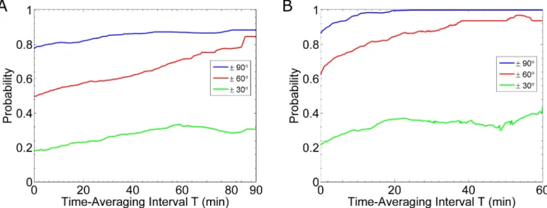
6C), we find there is an 86% probability the cell’s estimate is within 90˚ of the gradient’s true direction. After time-averaging for 10 minutes (Fig 6F), this probability increases to 97%.Fig 7shows how this probability for selected thresholds improves with time-averaging. In the case of fast reaction rates: kon= 1.6×10⁶(Ms)-1and koff= 0.011 s-1, we find that after about 20 min-utes of time-averaging, cells know the direction of the gradient within 90˚ (Fig 7B). In con-trast, for the case of slow reaction rates: kon= 1.6×10⁵(Ms)-1and koff= 0.0011 s-1, if a cell time-averages for 90 minutes, then the probability of being correct within 90˚ is only 88% (Fig 7A). Similarly, we find short lengths of time-averaging (e.g. less than 20 min) are more benefi-cial in the case of fast reaction rates than slow rates. That is, for 20min of time-averaging, a sys-tem with fast rates improves the probability of being accurate within 60˚ by 22%; whereas, a system with slow rates improves the probability of being accurate within 60˚ by only 8%.
Section III: Sensing during gradient formation
Formation of the gradient. We have thus far only considered steady state pheromone
gradients. We now study the Ste2distribution as the gradient forms across the cell. To simu-late a developing gradient (0.1 nM/μm), we fix the pheromone concentration at the x = 5μm boundary and enforce a partially absorbing boundary at x = –5μm. That is, we do not inject new molecules from the x = –5μm boundary, but reflect molecules that reach this boundary back into the computational domain with the appropriate probability to establish the desired
Fig 6. Estimated Angular Deviation from Gradient. Results from sixteen simulations of cells in a 0.1 nM/μm gradient, using the fast binding and unbinding rates: kon= 1.6×10⁶(Ms)-1and koff= 0.011 s-1. In this figure we plot the cell’s estimate of the gradient, gest, which is equal to the center of mass
of the Ste2*distribution. “Elevation” measures the angle of gestrelative to the x-y plane, and “Azimuthal” measures the counterclockwise angle in the x-y
plane away from the positive x-axis. The “Angular Deviation” is the angle between the true gradient and gest. (A) Trajectory in the azimuthal-elevation
phase plane of a single simulation. (B) Plots of the instantaneous angular deviation from sixteen cells. Each color represents a single simulation result. (C) Histogram of the data in (B). The average angle angular deviation is indicated by the vertical red line; the mean is 59.7˚. (D) Time-averaged (10 min) trajectories in the azimuthal-elevation phase plane of sixteen simulations. (E) Plots of the time-averaged angular deviation (10 min). (F) Histogram of the data in (E). The average angular deviation is indicated by the vertical red line; the mean is 47.8˚.
concentration at this boundary (seeMethods: “Gradient Method 2” for details).Fig 8Bshows the resulting steady state pheromone concentration profile in the absence of a cell. The inclu-sion of the cell boundary produces the pheromone concentration profile shown inFig 8A. Again, we find the presence of the cell sharpens the gradient similar to previous cases (Fig 4A and 4B). However, unlike previous cases, the concentration is not held constant at x = –5μm, and the final concentration at this boundary depends on the presence or absence of the cell.
Transient differences in receptor occupancy. Recent work suggests that the largest
difference in receptor occupancy (Δn = nfront−nback) occurs transiently, before the receptor-Fig 7. Time-averaging Gradient Prediction. Results for the probability that the cell’s prediction of the gradient is accurate within three thresholds: 90˚
(blue curves), 60˚ (red curves) and 30˚ (green curves). In all cases, we simulate cells in a 0.1 nM/μm gradient. (A) Results for slow binding kinetics. The curves are calculated from twenty-six simulations. (B) Results for fast binding kinetics. The curves are calculated from the same sixteen simulations used to generateFig 6.
doi:10.1371/journal.pcbi.1005386.g007
Fig 8. Steady-state Gradient Profiles when Molecules are only Injected from One Side. Pheromone molecules are added at the x = 5μm boundary and a partially absorbing boundary is placed at x = –5μm boundary (seeMethods: “Gradient Method 2”). (A) The steady state concentration profiles in the presence of a cell. We do not simulate any reactions. (B) The steady state concentration profile in the absence of a cell. Note that the presence of the cell sharpens the gradient and reduces the overall concentration behind the cell.
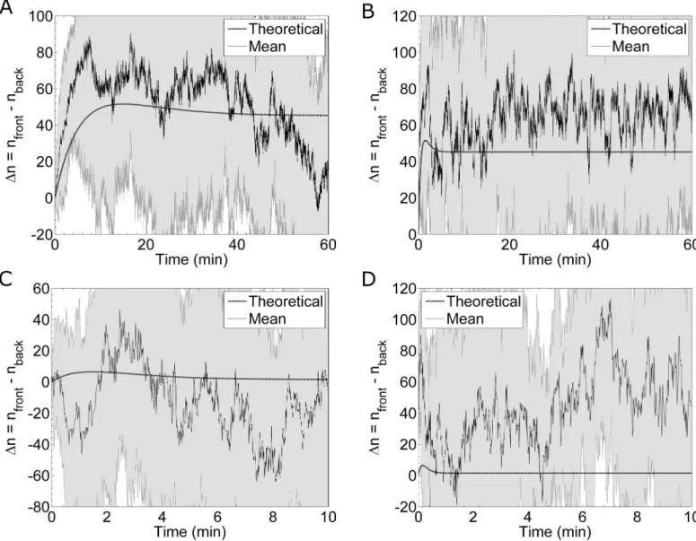
pheromone system comes to equilibrium [13]. The receptor-pheromone binding and unbind-ing rates determine when this peak difference occurs (Fig 9) [13]. The authors conclude this transient effect is significant enough to improve the gradient sensing ability of yeast cells dur-ing matdur-ing. Furthermore, they argue this effect is particularly relevant for gradient sensdur-ing in high background levels of pheromone [13]. To investigate this transient effect, we simulate a cell whose receptors are all initially unoccupied and, using the method discussed above, flow pheromone from one side. We simulate cells in a shallow gradient of 0.1 nM/μm under two different background concentrations: 6.9nM (which is the KDof the receptor) and 69nM (which is ten times the KDof the receptor). Additionally, we study fast and slow binding Fig 9. Transient Difference in Receptor Occupancy. Simulation results for the difference in receptor occupancy,Δn, between the front and back halves of a cell in a developing pheromone gradient of 0.1 nM/μm. The solid black lines are the meanΔn computed from simulations, and the shaded gray areas are the standard deviations from the means. The dashed black lines show the theoretical differences based on binding kinetics. (A) Results from twenty simulations of a system with slow binding kinetics in an average concentration of 6.9 nM. The theoretical curve is calculated using an average pheromone concentration of 6.775nM in the back half and 7.025nM in the front half. (B) Results from twenty simulations of a system with fast binding kinetics in an average concentration of 6.9nM. (C) Results from eight simulations of a system with slow binding kinetics in an average pheromone concentration of 69 nM. The theoretical curve is calculated using an average pheromone concentration of 68.875nM in the back half and 69.125nM in the front half. (D) Results from eight simulations of a system with fast binding kinetics in an average pheromone concentration of 69nM.
kinetics. For each of these cases,Fig 9shows the theoretical and simulatedΔn over time. Aver-aging over many simulations, we find the difference in occupancy is typically larger than theo-retically expected (Fig 9A, 9B and 9D). Thein silicoΔn is higher than theoretically expected, because the simulations, which account for the physical boundary of the cell, produces a sharper gradient than the ideal gradient assumed in the theoretical model. Because ourin silico model includes biophysical sources of noise, we can determine the fluctuations inΔn. These fluctuations appear much larger than the transient peak height in the theoretical model (Fig 9). Therefore, this transient effect is masked by the fluctuations in receptor occupancy.
As discussed above, by analyzing the Ste2distribution as two halves, we artificially intro-duce spatial information about the direction of the gradient in our analysis. A more appropri-ate measure of the Ste2distribution that can be computed for a forming gradient is the center of mass of all Ste2molecules. We interpret the direction of the resulting vector to be the cell’s estimate of the gradient’s direction. To construct a measure of the cell’s confidence in this esti-mate, we normalize the magnitude of this vector with respect to the fraction of active recep-tors:
Confidence¼1
R n NjhSte2
!
ij ð9Þ
where,Ris the radius of the cell,Nis the total number of receptors, andnis the number of active receptors. This confidence measure ranges between 0 and 1. A value near 0 indicates that either there are few active receptors or the active receptors are nearly uniformly distrib-uted. A confidence value of 1 indicates all the receptors are active and located in the same posi-tion. For comparison, a cell at equilibrium in a uniform pheromone concentration of 6.9nM, the confidence is6.4×10−3(S2 Text, Section D). In the case of slow reaction rates, we find
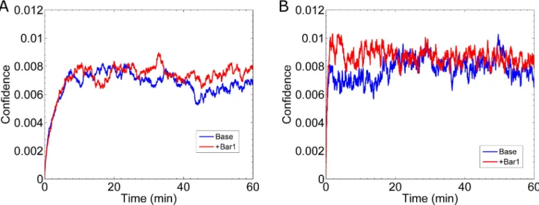
that the cell’s confidence reaches a maximum of 8×10⁻³around 20min (Fig 10A). In the case of fast reaction rates, the maximum confidence is again around 8×10⁻³and is reached slightly
Fig 10. Gradient Estimation During Formation of the Gradient. (A) Result for the cell’s confidence (Eq 9) in the direction of the gradient for slow binding kinetics. In these simulations the emerging gradient is 0.1 nM/μm with a mean of 6.9 nM. The blue curve, labeled “Base”, is for the case without Bar1, and the red curve, labeled “+Bar1”, includes the effect of Bar1. The “Base” data is the mean of the same twenty simulations fromFig 9A, and the “+Bar1” data is the mean of sixteen simulations. (B) Same as (A) except for fast kinetics. The “Base” data is the mean of the same twenty simulations fromFig 9B, and the “+Bar1” data is the mean from sixteen simulations.
later around 30 min (Fig 10B). These results further demonstrate that transient effects do not significantly improve gradient sensing.
Bar1 improves gradient sensing for fast reaction rates. It has been shown that the
pher-omone protease Bar1 can improve the gradient sensing ability of the cell by locally sharpening the gradient [4,5]. We model the Bar1 concentration as a static field. That is, the Bar1 con-centration is a function of the distance from center of the cell (seeMethods: “Bar1 Model”). Based on previous models, we set this concentration of Bar1 at the cell surface to be 0.85nM [5]. Away from the cell surface, this concentration decreases as1
r. At each time step, phero-mone molecules have a probability of being catalyzed based on the local concentration of Bar1. We use a catalytic rate of kcat= 2.5×10⁸(Ms)-1, which is based on a previous model [5].
In the case of slow reaction rates, the cell’s confidence (Fig 10A) is not significantly improved by the presence of Bar1. However, in the case of fast reaction rates, the cell’s confi-dence improves in the first 20 min to8.9×10−3with Bar1, as compared to 6.4×10⁻³without Bar1 (Fig 10B). Thus, if the true binding and unbinding rates are slow, as measured [8,12], then Bar1 does not effectively help an isolated cell determine the direction of a shallow gradient.
Discussion
Fluctuations in receptor occupancy
One potential mechanism for detecting chemical gradients is for cells to use the spatial distri-bution of active receptors. However, fluctuations in binding and release of ligand and receptor diffusion introduce significant uncertainty in receptor occupancy, making this task more diffi-cult. For a cell attempting to sense a shallow gradient, this uncertainty can mask the signal. For example, a cell with 10000 receptors in a shallow gradient of 0.1 nM/μm centered at the KDof the receptor, has a difference in occupancy between the front and back of the cell ofΔn
45± 50 [3]. This estimate does not include the effect of receptor diffusion, which further reduces the difference in receptor occupancy. Our results, which best match the theory of Berezhkovskii and Szabo [20], indicate that the effects from stochastic binding and unbinding are the largest source of variability in receptor occupancy.
Mechanisms for noise-reduction
Because the cell receives all information on the extracellular pheromone concentration from the Ste2 receptor, fluctuations in receptor occupancy represent the first major source of noise during gradient sensing. Downstream signaling events could generate additional sources of noise and/or act to amplify gradients in receptor occupancy. However, these effects are beyond the scope of our current investigation. Instead, we evaluated potential cellular mechanisms cells might employ to reduce noise from fluctuations in receptor occupancy.
Receptor endocytosis has also been suggested as a noise-reduction mechanism, because it removes ligand from the environment thereby eliminating noise from re-binding the same ligand molecule [6]. It may also serve to reduce noise due to receptor diffusion. To investigate the effects of endocytosis on gradient sensing, we adapted our model to absorb rather than release pheromone molecules. Contrary to expectations, we do not find any advantage to removing the ligand. That is, ligand absorption does not reduce the noise as compared to releasing ligand (Fig 3C and 3D).
The pheromone protease, Bar1, has also been suggested as a possible mechanism to im-prove gradient sensing. We implicitly modeled Bar1 as a concentration field, which radially decays away from the cell’s surface. Our results indicate that Bar1 does improve the cell’s abil-ity to sense an emerging gradient (Fig 10B). Specifically, during the first 20 min that a shallow gradient (0.1 nM/μm) forms around the cell, the presence of Bar1 increases the cell’s confi-dence in estimating the direction of the gradient. Curiously, our results predict this advantage only occurs if the reaction rates for Ste2 and pheromone are fast (kon= 1.6×10⁶(Ms)-1and koff= 0.011 s-1). This advantage may also be dependent upon other parameters, e.g. the con-centration of Bar1 near the cell and the catalytic rate of Bar1 on pheromone. Future work will be dedicated to studying how these parameters affect gradient sensing.
Gradient sharpening due to steric effects
Because we directly simulate diffusion, our method captures subtle effects in the distribution of pheromone, e.g. boundary effects from the cell membrane. Similar effects have been shown to play a significant role in other systems, for example in the arrangement of actin bundles in filopodia [28]. Here, we found that because the cell is impermeable to pheromone, it acts to sharpen the gradient (Figs4A and 4Band8). Importantly, we find this sharpening is reflected in the active receptor distribution (Figs4C and 4Dand9). Our simulation methods are analo-gous to some yeast gradient sensing experiments, in which a pheromone gradient is established by flowing two different concentrations of pheromone into a microfluidics chamber [5,26,29– 31]. In those experiments, it is not uncommon for multiple cells to be adjacent, e.g. as mother-daughter pairs or as multi-cell clusters. Our results suggest these adjacent cells experience a sharper than expected gradient. Additionally, we performed simulations using small (1.75μm radius) cells and found less gradient sharpening than with 2.5μm radius cells. Consequently, these cells had less of a difference in receptor occupancy (S2 Text, Section E). Our results
complement other work which corroborates this relationship between cell size and the cell’s ability to gradient sense [32].
Gradient sharpening is strongest if pheromone is injected into the computational domain from only one side. This arrangement is common in microfluidic gradient chambers [30,33]. Additional steric effects may also be present due to the microfluidic chambers themselves. For example, many microfluidic chambers have a height similar to a yeast cell (~5μm). Therefore, the presence of a cell severely impedes the flow of pheromone in the chamber and further sharpens the gradient. Hence experiments that aim to test the limit of gradient sensing (i.e. the shallowest gradient a cell can detect) must carefully consider steric effects from the cell itself, any adjacent neighbors and the experimental tools. These effects alter the gradient, such that the true gradient experienced by the cells is sharper than expected.
Tools for simulating gradients
stochastic diffusion simulations. These methods explain how many and how far to inject parti-cles into the simulation space per time step. We also capitalize on hardware acceleration via the use of GPGPUs to achieve massive parallelization. As a result we were able to simulate tens of thousands of molecules over billions of time steps.
Methods
Our goal is to develop a simulation platform that resolves individual signaling molecules in a continuous 3-dimensional space (Fig 1). It also should faithfully capture the stochastic proper-ties of diffusion of both the extracellular signaling molecules and receptors in the cell mem-brane, and of the biochemical reactions involved in ligand binding and release and receptor internalization (Fig 1A). For these reasons, we choose a Particle-Based Stochastic Reaction-Diffusion model in which molecules are modeled as point particles that can stochastically react and diffuse continuously in space.
Our simulation domain is a cubic volume with 10μm sides. We model the cell as a sphere at the center of the volume with a radius of 2.5μm (Fig 1B). The state of the system is defined by the position of all the molecules and chemical state of each receptor (bound or unbound). Pheromone molecules cannot be located inside the cell, and receptor molecules are restricted to the surface of the cell. Given the current state at time t0, we determine the subsequent state at time t0+Δt, whereΔt is a time step of fixed length, by calculating all binding reactions, unbinding reactions and diffusion of each molecule. A binding event occurs with probability Pbind(Table 1), if a pheromone molecule is within a distance of rbind= 4nm (binding radius) of an unbound receptor (Fig 1B.W). An unbinding event occurs during the time step,Δt, with probability Punbind(Table 1). A bound receptor releases a pheromone molecule a dis-tance of runbind= 4nm (unbinding radius) away at a randomly chosen angle (Fig 1B.W). During diffusion, each particle stochastically moves to a new position with appropriate con-ditions enforced at the boundaries of the computational domain and the cell (Fig 1B.X–1B. Z). The time step is chosen such that the length scale of pheromone diffusion ( ffiffiffiffiffiffiffiffiffiffiffiffiffi2DaDt
p
) is similar to the binding radius (4nm). We have performed extensive tests to validate all our simulation methods, including tests to demonstrate that: 1) diffusion produces the correct mean squared displacement; 2) first order reactions match theoretical decay curves, and 3) second order reactions match theoretical binding curves. We do not include these tests here, because each process has been extensively validated both theoretically and computationally by others [18], and we did not find our validations particularly insightful. On the microscopic scale, our model captures the stochasticity due to reactions and diffusion and monitors the exact position of all molecules in a 3D space. Below, we explain the microscopic rules that each molecule follows.
Binding reactions
In most particle-based reaction-diffusion simulations, a binding event is executed as follows. When a ligand molecule is nearby (within the binding radius of) an unbound receptor mole-cule, the ligand molecule is removed from the system, and the receptor molecule is switched to the ‘bound’ state. To match the macroscopic binding kinetics, the binding radius is calculated from the binding rate and the diffusion constants of the two molecular species:
rbind¼ kon
4pðDaþDSte2Þ
ð10Þ
rates reported in the literature using this method requires a binding radius on the order of Angstroms, which is much smaller than the size of Ste2 (GPCRs protrude about 4nm outside the cell membrane [35]). As discussed by Erban and Chapman the unrealistic binding radius results from the assumption that the binding probability is 100% [18]. That is, a ligand mole-cule within the binding radius of an unbound receptor binds with certainty. The model put forward by Erban and Chapman, removes this assumption and establishes a mathematical framework, in which the binding probability is a function of the binding radius [18,36]. That is, a ligand molecule within a specified binding radius binds with a probability that produces an average binding rate consistent with the macroscopic rate constant kon. We choose the binding radius to be 4nm and calculate the binding probability by numerically solving the fol-lowing system of equations derived by Erban and Chapman [36]:
konDt
rbind3
¼Pbind
Z 1
0
4pz2gðzÞdz ð11Þ
where,
gð Þ ¼^r ð1 PbindÞ
Z 1
0
Kð^r;^r0;g Þgð^r0
Þd^r0þ
Z 1
1
Kð^r;^r0;g Þgð^r0
Þd^r0þPbindKð^r;a;gÞ
a2
Z 1
0
gðzÞz2
dz
K z;z0 ;g
ð Þ ¼ z
0
zgpffiffiffiffiffiffi2p exp
ðz z0Þ2
2g2
exp ðzþz
0Þ2
2g2
a¼runbind
rbind
g¼
ffiffiffiffiffiffiffiffiffiffiffiffiffiffiffiffiffiffiffiffiffiffiffiffiffiffiffiffiffiffiffi
2ðDaþDSte2ÞDt
p
rbind
Using the values forΔt, kon, Dα, DSte2, rbindand runbindgiven inTable 1, a pheromone mole-cule has a 0.2% chance of binding. We provide a detailed description of how we calculate the probability in the Supplemental Methods (S1 Text, Section A).
Importantly, we note that to apply the method of Erban and Chapman to our system, we must double the binding probability. The probability calculated from their method is appro-priate when the ligand molecule can approach the receptor from any direction. However, in our system, the pheromone molecules can only approach the receptor from the outside of the cell. Therefore to achieve macroscopic rate constants consistent with experimental measure-ments, we double the binding probability. This adjustment was also used in recent work [37]. See the Supplemental Methods (S1 Text, Section A).
Unbinding reactions
Given a dissociation rate koff, we can calculate the probability, Punbind, that a ligand molecule dissociates from a ‘bound’ receptor in the time intervalΔt as follows:
Punbind¼1 exp½ koffDt ð12Þ
Diffusion of pheromone
Let (x(t), y(t), z(t)) be the current position at time t, then to diffuse a pheromone molecule in 3D, the new position (x(t +Δt), y(t +Δt), z(t +Δt)) is found from the following equations:
xðtþDtÞ ¼xðtÞ þZ1
ffiffiffiffiffiffiffiffiffiffiffi
2DDt
p
ð13aÞ
yðtþDtÞ ¼yðtÞ þZ2
ffiffiffiffiffiffiffiffiffiffiffi
2DDt
p
ð13bÞ
zðtþDtÞ ¼zðtÞ þZ3
ffiffiffiffiffiffiffiffiffiffiffi
2DDt
p
ð13cÞ
The Zis are independent random numbers drawn from a Gaussian distribution with a mean of 0 and a variance of 1. The new position is modified if it is located outside the simulation vol-ume or inside the cell. Reflecting boundary conditions are imposed at the four boundaries:y= ±5μm andz=±5μm (Fig 1B.X). Additionally, pheromone molecules reflect off the surface of the cell, because the cell membrane is impermeable to pheromone (Fig 1B.Y). Details for cal-culating the reflection off the cell surface are provided in the Supplemental Methods (S1 Text, Section B).
The last two boundaries,x=±5μm, are constructed to establish a linear pheromone gradi-ent along the x-axis. We describe two differgradi-ent methods for treating thex=±5μm boundaries. In method 1, each boundary has a fixed concentration. In method 2, one boundary has a fixed concentration while the other is partially absorbing. The next two sections describe the physi-cal interpretation and algorithmic implementation for each method.
Pheromone gradient method 1
−
fixed concentrations
In this method, we model a fixed concentration at each boundary. A gradient is formed when we set the concentration at one end of the computational domain higher than at the other. This method is consistent with the design of many microfluidic chambers used to study gradi-ent sensing [5,26,29–31]. To maintain a fixed concgradi-entration at each boundary, pheromone molecules are added to and removed from the simulation volume in processes called ‘injection’ and ‘ejection’, respectfully (Fig 1B.Z).
For ejection, we remove all pheromone molecules located outside the boundaries (x<– 5μm, orx>5μm) (Fig 1B.Z). For injection, we create a number of new pheromone molecules and position them near either thex= 5μm orx= –5μm boundary. On average, for a concen-trationcat the boundary, the number to inject at each time step is calculated using the equa-tion:
ninj ¼
0:6022 nMmm3ca
ffiffiffiffiffiffiffiffiffiffiffi
DaDt
p
r
ð14Þ
whereais the area of the boundary (100μm2for most of our simulations); Dαis the diffusion
constant for pheromone molecules, andΔτ is the elapsed time between two injection pro-cesses. The derivation ofEq 14is found in the Supplemental Methods (S1 Text, Section C).
1B.Z). The probability distribution function for the injection distance, dinj, is given by:
PðdinjÞ ¼
1
2 1 erf dinj
ffiffiffiffiffiffiffiffiffiffiffiffiffi
4DaDt
p
!
" #
ð15Þ
The derivation ofEq 15is provided in the Supplemental Material (S1 Text, Section C).
Be-cause it is computationally expensive to generate a random number from the distribution given byEq 15, we select a random value from a pre-calculated list. This list has more than 12 million random values whose distribution matchesEq 15. Further discussion for implement-ingEq 15is provided in the Supplemental Methods (S1 Text, Section C).
For computational efficiency, these two processes (injection and ejection) are implemented on a slightly coarser time scale,Δτ, than the time scale for diffusionΔt. It is important to note that ejection and injection must be calculated on the same time scale. Details and justification for the two time scales are discussed below in “Algorithm Overview”.
Pheromone gradient method 2 –partially absorbing boundary
In this method, we model a fixed concentration at one boundary (x= 5μm), while the other boundary (x= –5μm) is partially absorbing. We use this method to simulate the formation of a gradient from a source located at the positive x boundary (seeResultsSection III).
At thex= 5μm boundary, the average number of molecules to inject at each time step, ninj, is given by:
ninj¼
0:6022
nMmm3 cx¼5a
ffiffiffiffiffiffiffiffiffiffiffi
DaDt
p
r
þ1
2agDaDt
!
ð16Þ
The derivation ofEq 16is found in the Supplemental Methods (S1 Text, Section C). Note that
in addition to defining the desired concentration at the boundary,cx = 5, we also define the
desired gradient at the boundary:g.Eq 14is a special case ofEq 16, in which there is no gradi-ent (g= 0 nM/μm) outside our volume (x>5μm).
At thex= –5μm boundary, no new molecules are injected, and during ejection, not all mol-ecules located outside the boundary (x<–5μm) are removed. Instead, each pheromone mole-cule has a probability of being reflected back inside the volume; otherwise, the molemole-cule is removed. To achieve a steady state gradient ofg, the probability of reflection is given by:
PRef ¼1
g
cx¼ 5
ffiffiffiffiffiffiffiffiffi
1
pDaDt q
þ1
2g
ð17Þ
if and only if,
cx¼ 5
g
ffiffiffiffiffiffiffiffiffiffiffiffiffi
4DaDt
p
The derivation ofEq 17is found in the Supplemental Methods (S1 Text, Section C). The
con-centration,cx= –5, and gradient,g, are the steady state concentration and gradient at thex= –5μm boundary when no cell is present in the computational domain. In the presence of a cell the pheromone molecules coming from the opposite boundary must diffuse around the cell. Therefore in this situation the resulting concentration will be less thancx= –5, and the gradient will be steeper thang.