Deep Reinforcement Learning using Capsules in Advanced Game Environments

(1)

Deep Reinforcement Learning

using Capsules in Advanced

Game Environments

PER-ARNE ANDERSEN

SUPERVISORS

Morten Goodwin Ole-Christoffer Granmo Master’s Thesis University of Agder, 2018 Faculty of Engineering and Science

(2)

UiA

University of Agder Master’s thesis

Faculty of Engineering and Science Department of ICT

c

(3)

Abstract

Reinforcement Learning (RL) is a research area that has blossomed tremen-dously in recent years and has shown remarkable potential for artificial intelligence based opponents in computer games. This success is primar-ily due to vast capabilities of Convolutional Neural Networks (ConvNet), enabling algorithms to extract useful information from noisy environments. Capsule Network (CapsNet) is a recent introduction to the Deep Learning algorithm group and has only barely begun to be explored. The network is an architecture for image classification, with superior performance for clas-sification of the MNIST dataset. CapsNets have not been explored beyond image classification.

This thesis introduces the use of CapsNet for Q-Learning based game algo-rithms. To successfully apply CapsNet in advanced game play, three main contributions follow. First, the introduction of four new game environments as frameworks for RL research with increasing complexity, namely Flash RL, Deep Line Wars, Deep RTS, and Deep Maze. These environments fill the gap between relatively simple and more complex game environments available for RL research and are in the thesis used to test and explore the CapsNet behavior.

Second, the thesis introduces a generative modeling approach to produce artificial training data for use in Deep Learning models including CapsNets. We empirically show that conditional generative modeling can successfully generate game data of sufficient quality to train a Deep Q-Network well. Third, we show that CapsNet is a reliable architecture for Deep Q-Learning based algorithms for game AI. A capsule is a group of neurons that de-termine the presence of objects in the data and is in the literature shown to increase the robustness of training and predictions while lowering the amount training data needed. It should, therefore, be ideally suited for game plays. We conclusively show that capsules can be applied to Deep Q-Learning, and present experimental results of this method in the envi-ronments introduced. We further show that capsules do not scale as well as convolutions, indicating that CapsNet-based algorithms alone will not be able to play even more advanced games without improved scalability.

(4)

(5)

Glossary

AGI Artificial General Intelligence. 28 AI Artificial Intelligence. 3, 7, 28, 31, 43

ANN Artificial Neural Network. 9–14, 19, 20, 22, 30, 41, 53, 74

CapsNet Capsule Network. iii, xii, xiii, 5–7, 27, 35, 49, 53, 55, 75, 77–85, 88–90

CCDN Conditional Convolution Deconvolution Network. xi–xiii, 58–60, 63–65, 68, 70, 72, 74, 75, 87, 89–91

CGAN Conditional Generative Adversarial Network. 25

ConvNet Convolutional Neural Network. iii, xii, xiii, 4, 5, 14–16, 22, 25, 27, 53, 66, 75, 77–85, 87, 88

DDQN Double Deep Q-Learning. 23 DL Deep Learning. 9, 42

DNN Deep Neural Network. 10, 11

DQN Deep Q-Network. xii, xiii, 19, 20, 23, 48, 49, 56, 58, 64, 75, 77–85, 89, 90

DRL Deep Reinforcement Learning. 9, 12, 22, 28, 37, 38, 49, 87 FCN Fully-Connected Network. 15

GAN Generative Adversarial Networks. 8, 24–26 MDP Markov Decision Process. 9, 18

(10)

Glossary Glossary

MLP Multilayer Perceptron. 10

MSE Mean Squared Error. 12, 13, 58, 64, 68, 70, 74 ReLU Rectified Linear Unit. 11

RL Reinforcement Learning. iii, 3–9, 18, 19, 21, 26, 28–31, 35, 37, 38, 41, 42, 44–49, 51–53, 55, 58, 72, 74, 75, 87–91

RTS Real Time Strategy Games. 3, 5–7, 29, 43, 44, 87–90 SDG Stochastic Gradient Decent. 12, 13, 58, 65, 75

(11)

List of Figures

2.1 Deep Neural network with two hidden layers . . . 10

2.2 Single Perceptron . . . 10

2.3 Loss functions . . . 13

2.4 Convolutional Neural Network for classification . . . 14

2.5 Fully-Connected Neural Network for classification . . . 15

2.6 MAX and AVG Pooling operation . . . 16

2.7 Overview: Generative Model . . . 17

3.1 Illustration of Generative Adversarial Network Model . . . . 24

3.2 Illustration of Conditional Generative Adversarial Network Model . . . 25

4.1 Environment field of focus . . . 36

4.2 FlashRL: Architecture . . . 37

4.3 FlashRL: Frame-buffer Access Methods . . . 38

4.4 FlashRL: Available environments . . . 39

4.5 Deep Line Wars: Graphical User Interface . . . 40

4.6 Deep Line Wars: Game-state representation . . . 41

4.7 Deep Line Wars: Game-state representation using heatmaps . 41 4.8 Deep RTS: Graphical User Interface . . . 43

4.9 Deep RTS: Architecture . . . 44

4.10 Deep Maze: Graphical User Interface . . . 46

4.11 Deep Maze: State-space complexity . . . 47

4.12 Flappy Bird: Graphical User Interface . . . 48

5.1 Proposed Deep Reinforcement Learning ecosystem . . . 50

5.2 Architecture: gym-cair . . . 51

5.3 Capsule Networks: Parameter count for different input sizes . 54 5.4 Capsule Networks: Architecture . . . 55

5.5 Architecture: CCDN . . . 59

(12)

List of Figures List of Figures

6.2 CCDN: Deep Maze: Training Performance . . . 68

6.3 CCDN: FlashRL: Training Performance . . . 70

6.4 CCDN: Flappy Bird: Training Performance . . . 72

7.1 DQN-CapsNet: Deep Line Wars . . . 77

7.2 DQN-ConvNet: Deep Line Wars . . . 77

7.3 DQN-CapsNet: Deep RTS . . . 78

7.4 DQN-ConvNet: Deep RTS . . . 78

7.5 DQN-CapsNet: Deep Maze . . . 79

7.6 DQN-ConvNet: Deep Maze . . . 79

7.7 DQN-CapsNet: Flappy Bird . . . 80

7.8 DQN-ConvNet: Flappy Bird . . . 80

7.9 DQN-CapsNet: Agent building defensive due to low health in Deep Line Wars . . . 81

7.10 DQN-CapsNet: Agent attempting to find the shortest path in a 25_×25 Deep Maze . . . 82

(13)

List of Tables

2.1 Equations of activation function . . . 11

3.1 Summary of researched platforms . . . 29

4.1 Deep Line Wars: Representation modes . . . 42

4.2 Deep RTS: Player Resources . . . 44

5.1 Capsule Networks: Dimension Comparison . . . 53

5.2 Deep Q-Learning architectures in testbed . . . 56

5.3 Deep Q-Learning architectures . . . 57

5.4 Deep Q-Learning hyper-parameters . . . 57

5.5 Proposed prediction cycle for CCDN . . . 60

6.1 CCDN: Deep Line Wars . . . 67

6.2 CCDN: Deep Maze . . . 69

6.3 CCDN: FlashRL: Multitask . . . 71

6.4 CCDN: Flappy Bird . . . 73

7.1 DQN: Hyper-parameters . . . 76

7.2 Comparison of DQN-CapsNet, DQN-ConvNet, and Random accumulative reward (Higher is better) . . . 85

(14)

(15)

List of Publications

A. Towards a Deep Reinforcement Learning Approach for Tower Line Wars . . . 105 B. FlashRL: A Reinforcement Learning Platform for Flash Games . . 121

(16)

(17)

Part I

(18)

(19)

Chapter 1

Introduction

1.1 Motivation

Despite many advances in Artificial Intelligence (AI) for games, no universal Reinforcement Learning (RL) algorithm can be applied to advanced game environments without extensive data manipulation or customization. This includes traditional Real-Time Strategy (RTS) games such as Warcraft III, Starcraft II, and Age of Empires. RL has been applied to simpler games such as the Atari 2600 platform but is to the best of our knowledge not successfully applied to more advanced games. Further, existing game envi-ronments that target AI research are either overly simplistic such as Atari 2600 or complex such as Starcraft II.

RL has in recent years had tremendous progress in learning how to control agents from high-dimensional sensory inputs like images. In simple envi-ronments, this has been proven to work well [36], but are still an issue for advanced environments with large state and action spaces [34]. In envi-ronments where the objective is easily observable, there is a short distance between the action and the reward which fuels the learning [21]. This is because the consequence of any action is quickly observed, and then easily learned. When the objective is complicated, the game objectives still need to be mapped to a reward, but it becomes far less trivial [24]. For the Atari 2600 game Ms. Pac-Man this was solved through a hybrid reward architec-ture that transforms the objective to a low-dimensional representation [59].

(20)

1.1. Motivation Introduction

Similarly, the OpenAI’s bot is able to beat world’s top professionals at one versus one in DotA 2. It uses an RL algorithm and trains this with self-play methods, learning how to predict the opponents next move.

Applying RL to advanced environments is challenging because the algorithm must be able to learn features from a high-dimensional input, in order act correctly within the environment [15]. This is solved by doing trial and error to gather knowledge about the mechanics of the environment. This process is slow and unstable [37]. Tree-Search algorithms have been successfully applied to board games such as Tic-Tac-Toe and Chess, but fall short for environments with large state-spaces [8]. This is a problem because the grand objective is to use these algorithms in real-world environments, that are often complex by nature. Convolutional Neural Networks (ConvNet) [28] solves complexity problems but faces several challenges when it comes to interpreting the environment data correctly.

The primary motivation of this thesis is to create a foundation for RL re-search in advanced environments, Using generative modeling to train arti-ficial neural networks, and to use the Capsule Network architecture in RL algorithms.

(21)

1.2. Thesis definition Introduction

1.2 Thesis definition

The primary objective of this thesis is to perform Deep Reinforcement Learning using Capsules in Advanced Game Environments. The research is split into six goals following the thesis hypotheses.

1.2.1 Thesis Goals

Goal 1: Investigate the state-of-the-art research in the field of Deep Learn-ing, and learn how Capsule Networks function internally.

Goal 2: Design and develop game environments that can be used for research into RL agents for the RTS game genre.

Goal 3: Research generative modeling and implement an experimental architecture for generating artificial training data for games.

Goal 4: Research the novel CapsNet architecture for MNIST classification and combine this with RL problems.

Goal 5: Combine Deep-Q Learning and CapsNet and perform experiments on environments from Achievement 2.

Goal 6: Combine the elements of Goal 3 and Goal 5. The goal is to train an RL agent with artificial training data successfully.

1.2.2 Hypotheses

Hypothesis 1: Generative modeling using deep learning is capable of generating artificial training data for games with a sufficient quality.

Hypothesis 2: CapsNet can be used in Deep Q-Learning with comparable performance to ConvNet based models.

(22)

1.2. Thesis definition Introduction

1.2.3 Summary

The first goal of this thesis is to create a learning platform for RTS game research. Second, to use generative modeling to produce artificial training data for RL algorithms. The third goal is to apply CapsNets to Deep Reinforcement Learning algorithms. The hypothesis is that its possible to produce artificial training data, and that CapsNets can be applied to Deep Q-Learning algorithms.

(23)

1.3. Contributions Introduction

1.3 Contributions

This thesis introduces four new game environments, Flash RL1_,_{Deep Line}

Wars2_, _{Deep RTS}_{, and} _{Deep Maze}_{. These environments integrates well} with OpenAI GYM, creating a novel learning platform that targets Deep Reinforcement Learning for Advanced Games.

CapsNet is applied to RL algorithms and provides new insight on how Cap-sNet performs in problems beyond object recognition. This thesis presents a novel method that use generative modeling to train RL agents using arti-ficial training data.

There is to the best of our knowledge no documented research on using CapsNet in RL problems, nor are there environments specifically targeted RTS AI research.

1_{Proceedings of the 30}th_{Norwegian Informatics Conference, Oslo, Norway 2017}

2_{Proceedings of the 37}th_{SGAI International Conference on Artificial Intelligence,}

(24)

1.4. Thesis outline Introduction

1.4 Thesis outline

Chapter 2 provides preliminary background research for Artificial Neural Networks (2.1, 2.2), Generative Models (2.3), Markov Decision Process (2.4), and Reinforcement Learning (2.5).

Chapter 3 investigates the current state-of-the-art in Deep Neural Networks (3.1), RL (3.2), GAN (3.3) and Game environments (3.5).

Chapter 4 outlines the technical specifications for the new game environ-ments Flash RL (4.1), Deep Line Wars (4.2), Deep RTS (4.3), and Maze (4.4). In addition, a well established game environment (Section 4.5) is introduced to validate experiments conducted in this thesis.

Chapter 5 introduces the proposed solutions for the goals defined in Sec-tion 1.2. SecSec-tion 5.1 outlines how the environments are presented as a learning platform. Section 5.2 introduces the proposal to use Capsules in RL. Section 5.3 describes the Deep Q-Learning algorithm and the imple-mentations used for the experiments in this thesis. Finally, the artificial training data generator is outlined in Section 5.4.

Chapter 6 and 7 shows experimental results from the work presented in Chapter 5.

Chapter 8 concludes the thesis hypotheses and provides a summary of the work done in this thesis. Section 8.2 outlines the road-map for future re-search related to the thesis.

(25)

Chapter 2

Background

Deep Learning (DL) is a branch of machine learning algorithms that recently became popularized due to the exponential growth in available computing power. DL is unique in that it is designed to learn data representations, as opposed to task-specific algorithms. Methods from DL are frequently used in RL algorithms, creating a new branch called Deep Reinforcement Learning (DRL). Artificial Neural Networks (ANN) are used at its core, utilizing the most novel DL techniques to gain state-of-the-art capabilities. This chapter outlines background theory for topics related to the research performed later in this thesis. Section 2.1 shows how Artificial Neural works work, moving onto computer vision with Convolutional Neural Net-works in Section 2.2. Section 2.4 outlines the theory behind the Markov Decision Process (MDP) and how it is used in RL.

(26)

2.1. Artificial Neural Networks Background

2.1 Artificial Neural Networks

An Artificial Neural Network (ANN) is a computing system that is inspired by how the biological nervous systems, such as the brain, function [19]. ANNs are composed of an interconnected network of neurons that pass data to its next layer when stimulated by an activation signal. When a network consists of several hidden layers, it is considered a Deep Neural Network

(DNN). Figure 2.1 illustrates a Deep Multi-Layer Perceptron (MLP) with two hidden layers.

Figure 2.1: Deep Neural network with two hidden layers

Figure 2.2: Single Perceptron

f(x) =

1 if Pn_i₌₁(wi·xi) +b >0

0 otherwise (2.1)

MLPs are considered a network because they are composed of many different functions. Each of these functions is represented as a perceptron. The combination of these functions gives us the ability to represent complex and high-dimensional functions [19]. Figure 2.2 illustrates a single perceptron from an MLP wherex1, x2· · ·xnare inputs to the perceptron. Each of these

(27)

2.1. Artificial Neural Networks Background Name Equation TanH tanh(z) = 2 1+e−2z −1 Softmax σ(z)j = e zj PK k=1ezk for j= 1· · ·K Sigmoid f(z) = ₁₊1_e₋z

Rectified Linear Unit (ReLU) f(z) =

( 0 forz <0 z otherwise LeakyReLU f(z) = ( z ifz >0 0.01z otherwise Binary f(z) = ( 0 ifz <0 1 ifz_≥0 Table 2.1: Equations of activation function

intozn =xn·wn and z =Pni=1(zn) +b where b is the bias value and z is the perceptron value. In Figure 2.2, the perceptron has a binary activation function (Equation 2.1), the neuron produce the value 1 for allz above 1, and 0 otherwise. There are several different activation functions that can be used in a perceptron network, see Section 2.1.1.

2.1.1 Activation Functions

The purpose of an Activation function is often to introduce non-linearity into the network. It is proven that an DNN using only linear activations are equal to a single-layered network [42]. It is therefore natural to use non-linear activation functions in the hidden layers of an ANN if the goal is to predict non-linear functions. TanH and Rectified Linear Unit (ReLU) has proven to work well in ANNs [22, 39, 65], but there exist several other alternatives as illustrated in Table 2.1. Researchers do not understand to the full extent why an activation function works better for a particular problem and is why trial and error is used to find the best fit [33].

(28)

2.1. Artificial Neural Networks Background

2.1.2 Optimization

Optimization in ANNs is the process of updating the weights of neurons in a network. In the optimization process, a loss function is defined. This function calculates the error/cost value of the network at the output layer. The error value describes the distance between the ground truth and the predicted value. For the network to improve, this error is backpropagated

back through the network until each neuron has an error value that reflects its positive or negative contribution to the ground truth. Each neuron also calculates the gradient of its weights by multiplying output delta together with the input activation value. Weights are updated usingstochastic gra-dient descent (SDG), which is a method of gradually descending the weight loss until reaching the optimal value.

2.1.3 Loss Functions

To measure the inconsistency between the predicted value and the ground truth, a loss function is used in ANNs. The loss function calculates a positive number that is minimized throughout the optimization of the parameters1 (Section 2.1.2). A loss function can be any mathematical formula, but there exist several well established functions. The performance varies on the classification task.

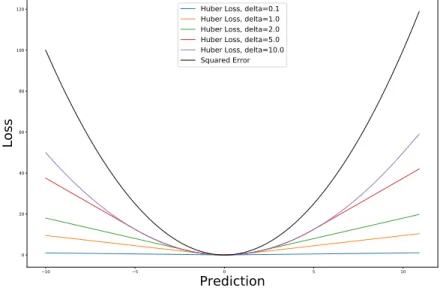
Mean Squared Error (MSE) is a quadratic loss function widely used in linear regression, and are also used in this thesis. Equation 2.2 is the standard form of MSE, where the goal is to minimize the residual squares (y(i)₋_y_ˆ(i)_). L= 1 n n X i=1 (y(i)₋_y_ˆ(i)₎2 _(2.2) Lδ(a) = ₁ 2a 2 _for_|_a_{| ≤}_δ, δ(_|a_{| −}1 2δ), otherwise (2.3)

Huber Loss is a loss function that is widely used in DRL. It is similar to MSE, but are less sensitive to data far apart from the ground truth. Equation 2.3 defines the function where a refers to the residuals and δ

(29)

2.1. Artificial Neural Networks Background 10 5 0 5 10

Prediction

0 20 40 60 80 100 120

Loss

Huber Loss, delta=0.1 Huber Loss, delta=1.0 Huber Loss, delta=2.0 Huber Loss, delta=5.0 Huber Loss, delta=10.0 Squared Error

Figure 2.3: Loss functions

refers to its sensitivity. Figure 2.3 illustrates the difference between MSE and Huber Loss using differentδ configurations.

2.1.4 Hyper-parameters

Hyper-parameters are tunable variables in ANNs. These parameters include learning rate, learning rate decay, loss function, and optimization algorithm like Adam, and SDG.

(30)

2.2. Convolutional Neural Networks Background

2.2 Convolutional Neural Networks

A Convolutional Neural Network is a novel ANN architecture that primarily reduces the compute power required to learn weights and biases for three-dimensional inputs. ConvNets are split into three layers:

1. Convolution layer 2. Activation layer 3. Pooling (Optional)

A Convolution layer has two primary components,kernel (parameters) and

stride. The kernel consists of a weight matrix that is multiplied by the input values in itsreceptive field. The receptive field is the area of the input that the kernel is focused on. The kernel then slides over the input with a fixed stride. The stride value determines how fast this sliding happens. With a stride of 1, the receptive field move in the direction x+ 1, and when at the end of the input x-axis,y+ 1.

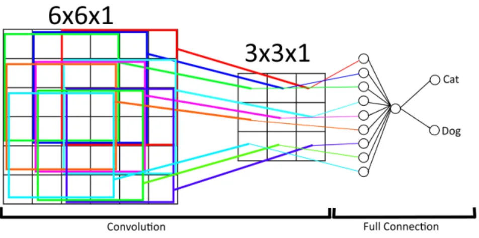
Figure 2.4: Convolutional Neural Network for classification

Consider a three-dimensional matrix representing an image of size 28×28×3. In this example, the goal is to classify the image to be either a cat or dog. By using hyperparameterskernel= 3×3 and stride= 1×1, there are 32

(31)

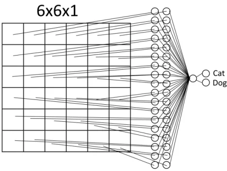
(FCN) with a single neuron layer, would have 2357 parameters to optimize. The reason why convolutions work is that it exploits what is calledfeature locality. ConvNets use filters that learn a specific feature of the input, for example, horizontal and vertical lines. For every convolutional layer added to the network, the information becomes more abstract, identifying objects and shapes. Figures 2.4 and 2.5 illustrate how a simple ConvNet is modeled compared to an FCN. The ConvNet use a stride of 1_×1 and a kernel size of 4_×4 yielding a 3_×3 output. This produces a total of 31 parameters to optimize, compared to 41 parameters in the FCN.

2.2.1 Pooling

Pooling is the operation of reducing the data resolution, often subsequent a convolution layer. This is beneficial because it reduces the number of parameters to optimize, hence decreasing the computational requirement. Pooling also controls overfitting by generalizing features. This makes the

(32)

network capable of better handling spatial invariance [48].

Figure 2.6: MAX and AVG Pooling operation

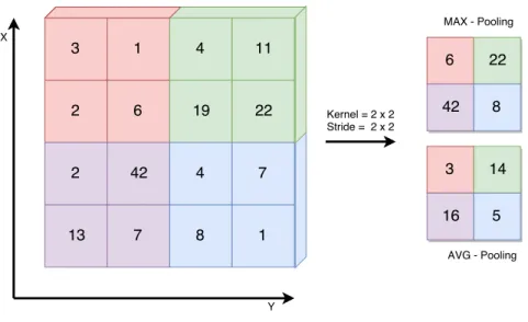
There are several ways to perform pooling. Max and Average pooling are considered the most stable methods in whereas Max pooling is most used in state-of-the-art research [29]. Figure 2.6 illustrates the pooling process using Max and Average pooling on a 4×4×X2 _{input volume. The} hyper-parameters for the pooling operation is kernel= 2_×2 and stride= 2_×2 applied to the input vector yields the resulting 2_×2_×X output volume. This operation performed independently for each depth slice of the input volume.

2.2.2 Summary

Historically, ConvNets drastically improved the performance of image recog-nition because it successfully reduced the number of parameters required, and at the same time preserving important features in the image. There are however several challenges, most notably that they are not rotation in-variant. ConvNets are much more complicated then covered in this section, but this beyond the scope of this thesis. For an in-depth survey of the ConvNet architecture, refer to Recent Advances in Convolutional Neural Networks [12].

2

(33)

2.3. Generative Models Background

Figure 2.7: Overview: Generative Model

2.3 Generative Models

Generative Models are a series of algorithms trying to generate an artificial output based on some input, often randomized. Generative Adversarial Networks and Variational Autoencoder is two methods that have shown excellent results in this task. These methods have primarily been used in generating realistic images from various datasets like MNIST and CIFAR-10. This section will outline the theory in understanding the underlying architecture of generative models.

The objective of most Generative Models is to generate a distribution of data, that is close to the ground-truth distribution (the dataset). The Gen-erative Model takes a Gaussian distributionz, as input, and outputs ˆp(x) as illustrated in Figure 2.7. The goal is to find parametersθthat best matches the ground truth distribution with the generated distribution. Convolu-tional Neural Networks are often used in Generative Modeling, typically for models using noise as input. The model has several hidden parameters θ

that is tuned via backpropagation methods like stochastic gradient descent. If the model reaches optimal parameters, ˆp(x) =p(x) is considered true.

(34)

2.4. Markov Decision Process Background

2.4 Markov Decision Process

MDP is a mathematical method of modeling decision-making within an

environment. An environment defines a real or virtual world, with a set of rules. This thesis focuses on virtual environments, specifically, games with the corresponding game mechanic limitations. The core problem of MDPs is to find an optimalpolicy function for the decision maker (hereby referred to as an agent). a |{z} Action = π(s) |{z}

Policy πfor states

(2.4)

Equation 2.4 illustrates how a decision/action is made using observed knowl-edge of the environmental state. The goal of the policy function is to find the decision that yields the best cumulative reward from the environment. MDP behaves like a Markov chain, hence gaining theMarkov Property. The Markov property describes a system where future states only depend on the present and not the past. This enables MDP based algorithms to do itera-tive learning [54]. MDP is the foundation of how RL algorithms operate to learn the optimal behavior in an environment.

(35)

2.5. Reinforcement Learning Background

2.5 Reinforcement Learning

Reinforcement learning is a process where an agent performs actions in an environment, trying to maximize some cumulative reward [53] (see Sec-tion 2.4). RL differs from supervised learning because the ground truth is never presented directly. In RL there are model-free and model-based

algorithms. In model-free RL, the algorithm must learn the environmen-tal properties (the model) without guidance. In contrast, model-based RL is defined manually describing the features of an environment [10]. For model-free algorithms, the learning only happens in present time and the future must be explored before knowledge about the environment can be learned [11, 26].

This thesis focuses on Q-Learning algorithms, a model-free RL technique that may potentially solve difficult game environments. This section inves-tigates the background theory of Q-Learning and extends this method to Deep Q-Learning (DQN), a novel algorithm that combines RL and ANN.

2.5.1 Q-Learning

Q-Learning is a model-free algorithm. This means that the MDP stays hid-den throughout the learning process. The objective is to learn the optimal policy by estimating the action-value functionQ∗(s, a), yielding maximum expected reward in state s performing action a in an environment. The optimal policy can then be found by

π(s) =argmaxaQ∗(s, a) (2.5)

Equation 2.5 is derived from finding the optimal utility of a state U(s) = maxaQ(s, a). Since the utility is the maximum value, the argmax of that

same value qualifies as the optimal policy. The update rule for Q-Learning is based on value iteration:

Q(s, a)_←Q(s, a)+_|{z}α LR R(s) |{z} Reward + γ |{z} Discount max_a0Q(s0, a0) | {z } New Q −Q(s, a) | {z } Old Q ! (2.6)

(36)

2.5. Reinforcement Learning Background

Equation 2.6 shows the iterative process of propagating back the estimated Q-value for each discrete time-step in the environment. α is the learning rate of the algorithm, usually low number between 0.001 and 0.00001. The reward function R(s) _∈ R, and is often between −1 < x < 1 to increase

learning stability. γ is the discount factor, discounting the importance of future states. The ”old Q” is the estimated Q-Value of the starting state while the ”new Q” estimates the future state. Equation 2.6 is guaranteed to converge towards the optimal action-value function, Qi →Q∗ as i→ ∞

[36, 53].

2.5.2 Deep Q-Learning

At the most basic level, Q-Learning utilizes a table for storing (s, a, r, s0) pairs. Instead, a non-linear function approximation can be used to approx-imate Q(s, a;θ). This is called Deep-Q Learning. θ describes tunable parameters (weights) for the approximation.ANNs are used as an approx-imation method for retrieving values from the Q-Table but at the cost of stability. Using ANN is much like compression found in JPEG images. The compression is lossy, and information is lost at compression time. This makes DQN unstable, since values may be wrongfully encoded under train-ing. In addition to value iteration, a loss function must be defined for the backpropagation process of updating the parameters.

L(θi) =E

h

(r+γmax_a0Q(s0, a0;θi)−Q(s, a;θi))2

i

(2.7) Equation 2.7 illustrates the loss function proposed by Minh et al [37]. It uses Bellmans equation to calculate the loss in gradient descent. To increase training stability,Experience Replay is used. This is a memory module that store memories from already explored parts of the state space. Experiences are often selected at random and then replayed to the neural network as training data. [36].

(37)

Chapter 3

State-of-the-art

This thesis focus on topics that are in active research, meaning that the state-of-the-art methods quickly advances. There have been many achieve-ments in Deep Learning, primarily related to Computer Vision topics. This chapter investigates recent advancements in Deep Learning (3.1), Deep Re-inforcement Learning (3.2), Generative Modeling (3.3), Capsule Networks (3.4) and Game Learning Platforms (3.5). In the success of Deep Learn-ing, there have been several breakthroughs in popular game environments. Section 3.6 outlines the state-of-the-art of applying RL algorithms to game environments.

(38)

3.1. Deep Learning State-of-the-art

3.1 Deep Learning

Deep Learning has a long history, dating back to late 1980’s. One of the first relevant papers on the area is Learning representations by backpropagating errors from Rumelhart et al. [44] In this paper, they illustrated that a deep neural network could be trained using backpropagation. The deep architecture proved that a neural network could successfully learn non-linear functions.

Yann LeCun started in the early 1990’s research into Convolutional Neu-ral Networks (ConvNet), with handwritten zip code classification as the primary goal [27]. He created the famous MNIST dataset, which is still widely used in the literature [28]. After ten years of research, LeCun et al. achieved state-of-the-art results on the MNIST dataset using ConvNets similar to those found in literature today [28]. But due to scaling issues with Deep ANNs, they were outperformed by classifiers like Support Vector Machines. It was not until 2006 with the paper A fast learning algorithm for deep belief nets by Hinton et al. that Deep Learning would appear again [17]. This paper showed how ectively train a deep neural network, by training one layer at a time. This was the beginning of Deep Neural Networks as they are known today.

For this thesis, Computer Vision is the most interesting architecture. There have been many advances in computer vision in the last couple of years. AlexNet [25], VGGNet [40] and ResNet [63] are models achieving state-of-the-art results in the ImageNet competition. These models are complex, but does a good job in image recognition. For DRL, there is to best of our knowledge no abstract model, that works for all environments. Therefore the model must be adapted to fit the environment at hand best.

(39)

3.2. Deep Reinforcement Learning State-of-the-art

3.2 Deep Reinforcement Learning

The earliest work found related to Deep Reinforcement Learning is Rein-forcement Learning for Robots Using Neural Networks. This PhD thesis illustrated how an ANN could be used in RL to perform actions in an envi-ronment with delayed reward signals successfully. [31]

With several breakthroughs in computer vision in early 2010’s, researchers started work on integrating ConvNets into RL algorithms. Q-Learning to-gether with Deep Learning was a game-changing moment, and has had tremendous success in many single agent environments on the Atari 2600 platform. Deep Q-Learning (DQN) as proposed by Mnih et al. used Con-vNets to predict the Q function. This architecture outperformed human expertise in over half of the games. [36]

Hasselt et al. proposedDouble DQN (DDQN), which reduced the overesti-mation of action values in the Deep Q-Network. This led to improvements in some of the games on the Atari platform. [7]

Wang et al. then proposed a dueling architecture of DQN which intro-duced estimation of the value function and advantage function. These two functions were then combined to obtain the Q-Value. Dueling DQN were implemented with the previous work of van Hasselt et al. [43].

Harm van Seijen et al. recently published an algorithm called Hybrid Reward Architecture (HRA) which is a divide and conquer method where several agents estimate a reward and a Q-value for each state. The algorithm per-formed above human expertise in Ms. Pac-Man, which is considered one of the hardest games in the Atari 2600 collection and is currently state-of-the-art in the reinforcement learning domain. The drawback of this algorithm is that generalization of Minh et al. approach is lost due to a huge number of separate agents that have domain-specific sensory input. [59]

There have been few attempts at using Deep Q-Learning on advanced sim-ulators made explicitly for machine-learning. It is probable that this is because there are very few environments created for this purpose.

(40)

3.3. Generative Modeling State-of-the-art

Figure 3.1: Illustration of Generative Adversarial Network Model

3.3 Generative Modeling

There are primarily three Generative models that are actively used in recent literature, GAN, Variational Autoencoders and Autoregressive Modeling. GAN show far better results than any other generative model and is the primary field of research for this thesis.

GAN show great potential when it comes to generating artificial images from real samples. The first occurrence of GAN was introduced in the paper

Generative Adversarial Networks from Ian J. Goodfellow et al. [23]. This paper proposed a framework using a generator and discriminator neural network. The general idea of the framework is a two-player game where the generator generates synthetic images from noise and tries to fool the discriminator by learning to create authentic images, see Figure 3.1. In future work, it was specified that the proposed framework could be ex-tended from p(x) → p(x | c). This was later proposed in the paper

(41)

Con-3.3. Generative Modeling State-of-the-art

Figure 3.2: Illustration of Conditional Generative Adversarial Network Model

ditional Generative Adversarial Nets (CGAN) by Mirza et al. [35]. GAN is extended to a conditional model by demanding additional informationy

as input for the generator and discriminator. This enabled to condition the generated images on information like labels illustrated in Figure 3.2. Radford et al. [33] proposed Deep Convolutional Generative Adversarial Networks (DCGAN) in Unsupervised Representation Learning with Deep Convolutional Generative Adversarial Networks. This paper improved on using ConvNets in unsupervised settings. Several architectural constraints were set to make training of DCGAN stable in most scenarios. This pa-per illustrated many great examples of images generated with DCGAN, for instance, state-of-the-art bedroom images.

In summer 2016, Salimans et al. (Goodfellow) presented Improved Tech-niques for Training GANs achieving state-of-the-art results in the classifi-cation of MNIST, CIFAR-10, and SVHN [46]. This paper introduced mini-batch discrimination, historical averaging, one-sided label smoothing and

(42)

3.3. Generative Modeling State-of-the-art

virtual batch normalization.

There have been many advances in GAN between and after these papers. Throughout the research process of GANs, the most prominent architecture for our problem is Conditional GANs which enables us to condition the input variable x on variable y. The most recent paper on this topic is Towards Diverse and Natural Image Descriptions via a Conditional GAN from Dai et al. [9]. This paper focuses on captioning images using Conditional GANs. It produced captions that were of similar quality to human-made captions. In RL terms it is successfully able to learn a good policy for the dataset.

(43)

3.4. Capsule Networks State-of-the-art

3.4 Capsule Networks

Capsule Neural Networks (CapsNet) is a novel deep learning architecture that attempts to improve the performance of image and object recognition. CapsNet is theorized to be far better at detecting rotated objects and re-quires less training data than traditional ConvNet. Instead of creating deep networks like for example ResNet-50, a Capsule layer is created, containing several sub-layers in depth. Each of these capsules has a group of neurons, where the objective is to learn a specific object or part of an object. When an image is inserted into the Capsule Layer, an iterative process of identi-fying objects begins. The higher dimension layers receive a signal from the lower dimensions. The higher dimension layer then determines which signal is the strongest and a connection is made between the winning signal (bet-ting). This method is called dynamic routing. This routing-by-agreement ensures that features are mapped to the output, and preserves all input information at the same time.

Pooling in ConvNet is also a primitive form of routing, but information about the input is lost in the process. This makes pooling much more vulnerable to attacks compared to dynamic routing. In current state-of-the-art, CapsNet is explained as inverse graphics, where a capsule tries to learn an activity vector describing the probability that an object exists. Capsule Networks are still only in infancy, and there is not well-documented research on this topic yet apart from state-of-the-art paper Dynamic Rout-ing Between Capsules by Sabour et al. [45].

(44)

3.5. Game Learning Platforms State-of-the-art

3.5 Game Learning Platforms

There exists several exciting game learning platform used to research state-of-the-art AI algorithms. The goal of these platforms is generally to provide the necessary platform for studying Artificial General Intelligence (AGI). AGI is a term used for AI algorithms that can perform well across several environments without training. DRL is currently the most promising branch of algorithms to solve AGI.

Bellemare et al. provided in 2012 a learning platform Arcade Learning Environment (ALE) that enabled scientists to conduct edge research in general deep learning [4]. The package provided hundreds of Atari 2600 environments that in 2013 allowed Minh et al. to do a breakthrough with Deep Q-Learning and A3C. The platform has been a critical component in several advances in RL research. [32, 36, 37]

The Malmo project is a platform built atop of the popular gameMinecraft. This game is set in a 3D environment where the object is to survive in a world of dangers. The paper The Malmo Platform for Artificial Intelli-gence Experimentation by Johnson et al. claims that the platform had all characteristics qualifying it to be a platform for AGI research. [20]

ViZDoom is a platform for research in Visual Reinforcement Learning. With the paper ViZDoom: A Doom-based AI Research Platform for Visual Re-inforcement Learning Kempka et al. illustrated that an RL agent could successfully learn to play the gameDoom, a first-person shooter game, with behavior similar to humans. [41]

With the paper DeepMind Lab, Beattie et al. released a platform for 3D navigation and puzzle solving tasks. The primary purpose of Deepmind Lab is to act as a platform for DRL research. [3]

In 2016, Brockman et al. from OpenAI released GYM which they referred to as ”a toolkit for developing and comparing reinforcement learning al-gorithms”. GYM provides various types of environments from following technologies: Algorithmic tasks, Atari 2600, Board games, Box2d physics engine, MuJoCo physics engine, and Text-based environments. OpenAI also hosts a website where researchers can submit their performance for compar-ison between algorithms. GYM is open-source and encourages researchers to add support for their environments. [5]

(45)

3.5. Game Learning Platforms State-of-the-art

Platform Diversity AGI Advanced Environment(s)

ALE Yes Yes No

Malmo Platform No No Yes

ViZDoom No Yes Yes

DeepMind Lab No No Yes

OpenAI Gym Yes Yes No

OpenAI Universe Yes Yes Partially

ELF No No Yes

(GYM-CAIR) Yes Yes Yes

Table 3.1: Summary of researched platforms

OpenAI recently released a new learning platform called Universe. This environment further adds support for environments running inside VNC. It also supports running Flash games and browser applications. However, despite OpenAI’s open-source policy, they do not allow researchers to add new environments to the repository. This limits the possibilities of running any environment. Universe is, however, a significant learning platform as it also has support for desktop games like Grand Theft Auto IV, which allow for research in autonomous driving [30].

Very recently Extensive Lightweight Flexible (ELF) research platform was released with the NIPS paperELF: An Extensive, Lightweight and Flexible Research Platform for Real-time Strategy Games. This paper focuses on RTS game research and is the first platform officially targeting these types of games. [58]

3.5.1 Summary

Multiple interesting observations about current state-of-the-art in learning platforms for RL algorithms were found during our research. Table 3.1 describes the capabilities of each of the learning platform in the interest of fulfilling the requirements of this thesis. GYM-CAIR is included in this comparison and is further described in Chapter 4 and 5.

(46)

3.6. Reinforcement Learning in Games State-of-the-art

3.6 Reinforcement Learning in Games

Reinforcement Learning for games is a well-established field of research and is frequently used to measure how well an algorithm can perform within an environment. This section presents some of the most important achieve-ments in Reinforcement Learning.

TD-Gammon is an algorithm capable of reaching an expert level of play in the board game Backgammon [56, 57]. The algorithm was developed by Gerald Tesauro in 1992 at IBM’s Thomas J. Watson Research Center. TD-Gammon consists of a three-layer ANN and is trained using an RL technique calledTD-Lambda. TD-Lambda is a temporal difference learning algorithm invented by Richard S. Sutton [52]. The ANN iterates over all possible moves the player can perform and estimates the reward for that particular move. The action that yields the highest reward is then selected. TD-Gammon is one of the first algorithms to utilize self-play methods to improve the ANN parameters.

In late 2015, AlphaGO became the first algorithm to win against a human professional Go player. AlphaGO is an RL framework that uses Monte Carlo Tree search and two Deep Neural Networks for value and policy esti-mation [49]. Value refers to the expected future reward from a state assum-ing that the agent plays perfectly. The policy network attempts to learn which action is best in any given board configuration. The earliest versions of AlphaGO used training data from games played by human professionals. In the most recent version, AlphaGO Zero, only self-play is used to train the AI [51] In a recent update, AlphaGO was generalized to work for Chess and Shogi (Japanese Chess) only using 24 hours to reach superhuman level of play [50]

DOTA 2 is an advanced player versus player game where the player is con-trolling a hero unit. The game objective is to defeat the enemy heroes and destroy their base. In August 2017, OpenAI invented an RL based AI that defeated professional players in one versus one game. Training was done only using self-play, and the algorithm learned how to exploit game mechanics to perform well.

DeepStack is an algorithm that can perform an expert level play in Texas Hold’em poker. This algorithm uses tree-search in conjunction with neu-ral networks to perform sensible actions in the game [38]. DeepStack is

(47)

3.6. Reinforcement Learning in Games State-of-the-art

a general-purpose algorithm that aims to solve problems with imperfect information.

There have been several other significant achievements in AI, but these are not directly related to the use of RL algorithms. These include Deep Blue1 and Watson from IBM.

(48)

(49)

Part II

(50)

(51)

Chapter 4

Environments

Simulated environments are a popular research method to conduct exper-iments on algorithms in computer science. These simulated environments are often tailored to the problem, and quickly proves, or disproves the capa-bility of an algorithm. This chapter proposes four new game environments for deep learning research: FlashRL,Deep Line Wars,Deep RTS, andDeep Maze. The game Flappy Bird is introduced as a validation environment for experiments conducted in Chapter 7. Figure 4.1 illustrates that each of these environments has different goals, and the agent placed in these envi-ronments are challenged in several topics, for instance, multitasking, deep and shallow state interpretation and planning. This chapter creates a foun-dation for research into CapsNet based RL-algorithms in advanced game environments.

(52)

Environments

(53)

4.1. FlashRL Environments

4.1 FlashRL

Adobe Flash is a multimedia software platform used for the production of applications and animations. The Flash run-time was recently declared deprecated by Adobe, and by 2020, no longer supported. Flash is still fre-quently used in web applications, and there are countless games created for this platform. Several web browsers have removed the support for the Flash runtime, making it difficult to access the mentioned game environments. Flash games are an excellent resource for machine learning benchmarking, due to size and diversity of its game repository. It is therefore essential to preserve the Flash run-time as a platform for RL.

Flash Reinforcement Learning(FlashRL) is a novel platform that acts as an input/output interface between Flash games and DRL algorithms. FlashRL enables researchers to interface against almost any Flash-based game envi-ronment efficiently.

Figure 4.2: FlashRL: Architecture

The learning platform is developed primarily for Linux based operating sys-tems but is likely to run on Cygwin with few modifications. There are several key components that FlashRL uses to operate adequate, see Figure 4.2. FlashRL uses XVFB to create a virtual frame-buffer. The frame-buffer acts like a regular desktop environment, found in Linux desktop distribu-tions [18]. Inside the frame-buffer, a Flash game chosen by the researcher is executed by a third-party flash player, for example, Gnash. A VNC server serves the frame-buffer and enable FlashRL to access display, mouse

(54)

and keyboard via the VNC protocol. The VNC Client pyVLC was spe-cially made for this FlashRL. The code base originates from python-vnc-viewer [55]. The last component of FlashRL is the Reinforcement Learning API that allows the developer to access the input/output of the pyVLC. This makes it easy to develop sequenced algorithms by using API callbacks or invoke commands manually with threading.

Figure 4.3: FlashRL: Frame-buffer Access Methods

Figure 4.3 illustrates two methods of accessing the frame-buffer from the Flash environment. Both approaches are sufficient to perform RL, but each has its strengths and weaknesses. Method 1 sends frames at a fixed rate, for example at 60 frames per second. The second method does not set any restrictions of how fast the frame-buffer can be captured. This is preferable for developers that do not require images from fixed time-steps because it demands less processing power per frame. The framework was developed with deep learning in mind and is proven to work well with Keras and Tensorflow [1].

There are close to a thousand game environments available for the first version of FlashRL. These game environments were gathered from different sources on the world wide web. FlashRL has a relatively small code-base and to preserve this size, the Flash repository is hosted at a remote site. Because of the large repository, not all games have been tested thoroughly. The game quality may therefore vary. Figure 4.4 illustrates tested games that yield a great value for DRL research.

(55)

(56)

4.2. Deep Line Wars Environments

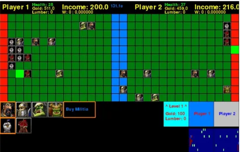
Figure 4.5: Deep Line Wars: Graphical User Interface

4.2 Deep Line Wars

The game objective of Deep Line Wars is to invade the opposing player (hereby enemy) with mercenary units until all health points are depleted (see Figure 4.5). For every friendly unit that enters the red area on the map, the enemy health pool is reduced by one. When a player purchases a mercenary unit, it spawns at a random location inside the red area of the owners base. Mercenary units automatically move towards the enemy base. To protect the base, players can construct towers that shoot projectiles at the opponents mercenaries. When a mercenary dies, a fair percentage of its gold value is awarded to the opponent. When a player sends a unit, the income is increased by a percentage of the units gold value. As a part of the income system, players gain gold at fixed intervals. [2]

To successfully master game mechanics of Deep Line Wars, the player (agent) must learn

• offensive strategies of spawning units,

(57)

Figure 4.6: Deep Line Wars: Game-state representation

Figure 4.7: Deep Line Wars: Game-state representation using heatmaps • maintain a healthy balance between offensive and defensive to

maxi-mize income

The game is designed so that if the player performs better than the opponent in these mechanics, he is guaranteed to win over the opponent.

Because the game is specifically targeted towards RL research, the game-state is defined as a multi-dimensional matrix. This way, it is trivial to input the game-state directly into ANN models. Figure 4.6 illustrates how the game state is constructed. This state is later translated into graphics, seen in Figure 4.5. It is beneficial to directly access this information because it requires less data preprocessing compared to using raw game images. Deep Line Wars also features abstract state representation using heat-maps,

(58)

Representation Matrix Size Data Size

Image 800_·600_·3 1440000

Matrix 10_·15_·5 750

Heatmap RGB 10_·15_·3 450

Heatmap Grayscale 10_·15_·1 150

Table 4.1: Deep Line Wars: Representation modes

seen in Figure 4.7. By using heatmaps, the state-space is reduced by a magnitude, compared to raw images. Heatmaps can better represent the true objective of the game, enabling faster learning for RL algorithms [47]. In Deep Line Wars, there are primarily four representation modes avail-able for RL.Tavail-able 4.1 shows that there is considerably lower data size for grayscale heatmaps. Effectively, the state-space can be reduced by 9600%, when no data preprocessing is done. Heatmaps seen in 4.7 define

• red pixels as friendly buildings, • green pixels as enemy units, and • teal pixels as the mouse cursor.

When using grayscale heatmaps, RGB values are squashed into a one-dimensional matrix with values ranging between 0 and 1. Economy drasti-cally increases the complexity of Deep Line Wars, and it is challenging to present only using images correctly. Therefore a secondary data structure is available featuring health, gold, lumber, and income. This data can then be feed into a hybrid DL model as an auxiliary input [61].

(59)

4.3. Deep RTS Environments

4.3 Deep RTS

RTS games are considered to be the most challenging games for AI algo-rithms to master [60]. With colossal state and action-spaces, in a continuous setting, it is nearly impossible to estimate the computational complexity of games such as Starcraft II.

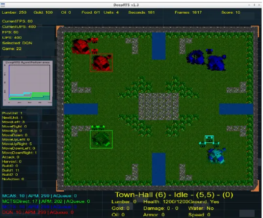
The game objective of Deep RTS is to build a base consisting of a Town-Hall and then expand the base to gain the military power to defeat the opponents. Each of the players starts with a worker. Workers can construct buildings and gather resources to gain an economic advantage.

Figure 4.8: Deep RTS: Graphical User Interface

The game mechanics consist of two main terminologies, Micro and Macro

management. The player with the best ability to manage their resources, military, and defensive is likely to win the game. There is a considerable

(60)

Player Resources

Property: Lumber Gold Oil Food Units

Value Range: 0 - 106 _{0 - 10}6 _{0 - 10}6 _{0 - 200} _{0 - 200} Table 4.2: Deep RTS: Player Resources

Figure 4.9: Deep RTS: Architecture

leap from mastering Deep Line Wars to Deep RTS, much because Deep RTS features more than two players.

The game interface displays relevant statistics meanwhile a game session is running. These statistics show the action distribution, player resources,

player scoreboard and a live performance graph. The action distribution keeps track of which actions a player has performed in the game session. These statistics are stored to the hard-drive after a game has reached the terminal state. Player Resources (Table 4.2), are shown at the top bar of the game. Player Scoreboard indicates the overall performance of each of the players, measured by kills, defensive points, offensive points and resource count. Deep RTS features several hotkeys for moderating the game-settings like game-speed and state representation. The hotkey menu is accessed by pressing the G-hotkey.

Deep RTS is an environment developed as an intermediate step between Atari 2600 and the famous game Starcraft II. It is designed to measure the performance in RL algorithms, while also preserving the game goal. Deep RTS is developed for high-performance simulation of RTS scenarios. The

(61)

game engine is developed in C++ for performance but has an API wrapper for Python, seen in Figure 4.9. It has a flexible configuration to enable different AI approaches, for instance online and offline RL. Deep RTS can represent the state as raw game images (C++) and as a matrix, which is compatible with both C++ and Python.

(62)

4.4. Deep Maze Environments

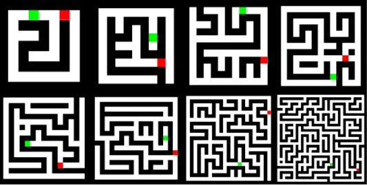
Figure 4.10: Deep Maze: Graphical User Interface

4.4 Deep Maze

Deep Maze is a game environment designed to challenge RL agents in the

shortest path problem. Deep Maze defines the problem as follows:

• How can the agent optimally navigate through any fully-observable maze?

The environment is simple, but becomes drastically more complicated when the objective is to find the optimal policyπ?(s) where s = state for all the maze configurations.

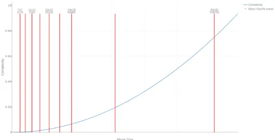
There are multiple difficulty levels for Deep Maze in two separate modes; deterministic and stochastic. In the deterministic mode, the maze structure is never changed from game to game. Stochastic mode randomizes the maze structure for every game played. There are multiple size configurations, ranging from 7_×7 to 55_×55 in width and height, seen in Figure 4.10. Figure 4.11 illustrates how the theoretical maximum state-space set S of Deep Maze increase with maze size. This is calculated by performing fol-lowing binomial: S = width×height_player₊_goal = w×h₂ . This is however reduced depending on the maze composition, where dense maze structures are

(63)

gen-4.4. Deep Maze Environments

Figure 4.11: Deep Maze: State-space complexity erally less complex to solve theoretically.

The simulation is designed for performance so that each discrete time step is calculated with fewest possible CPU cycles. The simulation is estimated to run at 3 000 000 ticks per second with modern hardware. This allows for fast training of RL algorithms.

From an RL point of view, Deep Maze challenges an agent in state-interpretation and navigation, where the goal is to reach the terminal state in fewest pos-sible time steps. It’s a flexible environment that enables research in a single environment setting, as well as multiple scenarios played in sequence.

(64)

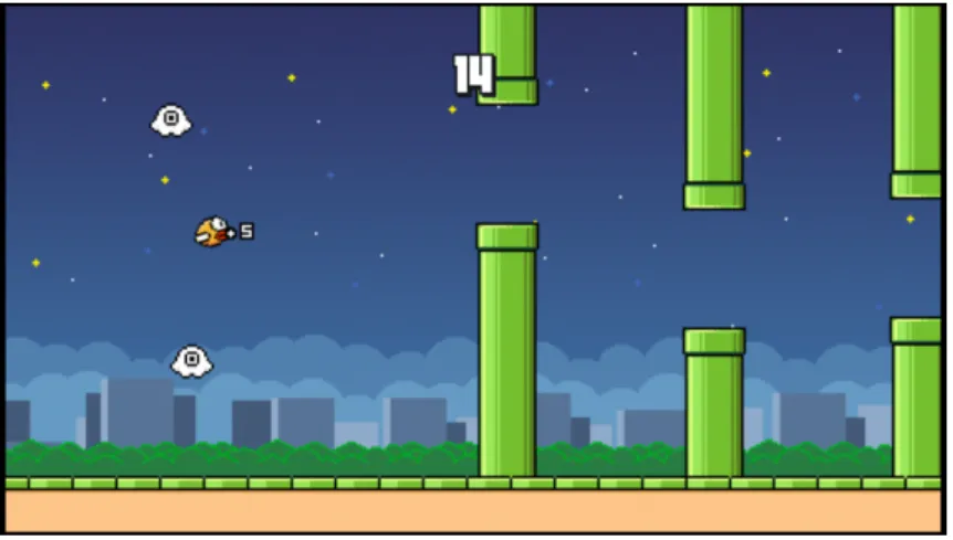
4.5. Flappy Bird Environments

Figure 4.12: Flappy Bird: Graphical User Interface

4.5 Flappy Bird

Flappy Bird is a popular mobile phone game developed by Dong Nguyen in May 2013. The game objective is to control a bird by ”flapping” its wings to pass pipes, see Figure 4.12. The player is awarded one point for each pipe passed.

Flappy Bird is widely used in RL research and was first introduced inDeep Reinforcement Learning for Flappy Bird [6]. This report shows superhuman agent performance in the game using regular DQN methods1_.

OpenAI’s gym platform implements Flappy Bird through PyGame Learning Environment2_{(PLE). It supports both visual and non-visual state} represen-tation. The visual representation is an RGB image while the non-visual in-formation includes vectorized data of the birds position, velocity, upcoming pipe distance, and position.

Figure 4.12 illustrates the visual state representation of Flappy Bird. It is represented by an RGB Image with the dimension of 512_×288. It is rec-ommended that raw images are preprocessed to gray-scale and downscaled to 80×80. Flappy Bird is an excellent environment for RL and provides adequate validation of new game environments introduced in this thesis.

1_{Source code:} _{https://github.com/yenchenlin/DeepLearningFlappyBird} 2_{Available at:}

(65)

Chapter 5

Proposed Solutions

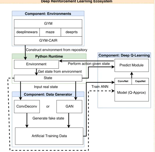
Three key solutions are presented in this thesis. First is an architecture that provides a generic communication interface between the environments and the DRL agents. Second is to apply Capsule Layers to DQN, enabling the research into CapsNet based RL algorithms. The third is a novel technique for generating artificial training data for DQN models. These components propose a DRL ecosystem that is suited for research purposes, see Figure 5.1.

(66)

Proposed Solutions

(67)

5.1. Environments Proposed Solutions

Figure 5.2: Architecture: gym-cair

5.1 Environments

OpenAI GYM is an open-source learning platform, exposing several game environments to the AI research community. There are many existing games available, but these are too simple because they have too easy game objec-tives. A game environment isregistered to the GYM platform by defining a

scenario. This scenario predefines the environment settings that determines the complexity. This type of registration is beneficial because it enables to construct multiple scenarios per game environment. An example of this would be the Maze environment, which contains scenarios fordeterministic

andstochastic gameplay for the different maze sizes.

Figure 5.2 illustrates how the environment ecosystem is designed using Ope-nAI GYM. Environments are registered to the GYM(1) platform.

Deep Line Wars(2), Deep RTS(3) and Maze(4) are then added to a common repository, called gym-cair₍₅₎. This repository links together all environ-ments, which can be imported via Python(6).

The benefit of using GYM is that all environments are constrained to a generic RL interface, seen in Algorithm 1. The environment is initially reset by runninggym.reset function (Line 1). It is assumed that the environment does not start in a terminal state (Line 2). While the environment is not in a terminal state, the agent can perform actions (Line 5 and 6). This procedure is repeated until the environment reaches the terminal state. By using this setup, it is far more trivial to perform experiments in the proposed environments. It also enables better comparison, because GYM

(68)

5.1. Environments Proposed Solutions

Algorithm 1 Generic GYM RL routine

1: statex=gym.reset

2: terminal=F alse

3: whilenot terminaldo

4: env.render

5: a=env.action space.sample

6: statex+1, rx+1, terminal, inf o=env.step(a)

7: statex =statex+1

8: end while

ensures that the environment configuration is not altered while conducting the experiments.

(69)

5.2. Capsule Networks Proposed Solutions

Layer Name Output Params Output Params

Input 28_×28_×1 0 84_×84_×1 0 Conv Layer 20×20×256 20 992 76×76×256 20 992 Primary Caps 6_×6_×256 5 308 672 34_×34_×256 5 308 672 Capsule Layer 16_×16 2 359 296 16_×16 75 759 616 Output 16 0 16 0 Parameters 7 688 960 81 089 280

Table 5.1: Capsule Networks: Dimension Comparison

5.2 Capsule Networks

Capsule Networks recently illustrated that a shallow ANN could successfully classify the MNIST dataset of digits, with state-of-the-art results, using considerably fewer parameters then in regular ConvNets. The idea behind CapsNet is to interpret the input by identifyingparts of the whole, namely the objects of the input. [45] The objects are identified using Capsules that have the responsibility of finding specific objects in the whole. A capsule becomes active when the object it searches for exist.

It becomes significantly harder to use CapsNet in RL. The objective of RL is to identify actions that are sensible to do in any given state. This means that actions become parts, and the whole becomes the state. Instead of classifying objects, the capsules now estimate a vector of the likelihood that an action is sensible to do in the current state.

Several issues need to be solved for CapsNet to work properly in the envi-ronments outlined in Chapter 4. The first problem is the input size. The MNIST dataset of digits contains images of 28×28×1 pixels, in contrast, game environments usually range between 64×64×1 and 128×128×3 pixels.

Table 5.1 illustrates the consequence of increasing the input size beyond the specified 28_×28_×1. By increasing the input size by a magnitude of 3 (84×84), the model gains over 10×parameters. Figure 5.3 illustrates how parameters increase exponentially with the input size. In attempts to solve the scalability issue, several Convolutional Layers can be put in front of the CapsNet. This enables the algorithm to extract feature maps from the original input, but it is crucial to not utilize any form of pooling prior the

(70)

P

arameter

s

(71)

Figure 5.4: Capsule Networks: Architecture

Capsule Layer. The whole reason to use Capsules is that it solves several problems with invariance that max-pooling possess.

Figure 5.4 illustrates how a standard CapsNet is structured, using a single Convolutional Layer. When a neural network is used, a question is defined to instruct the neural network to predict an answer. For a simple image classification task, the question is: what do you see in the image. The neural network then tries to answer, by using its current knowledge: I see a bird. The answer is then revealed to the neural network, which allows it to tune its response if it answered incorrectly. The same analogy can be used in an RL problem.

The hope is that despite having several scalability issues, it is possible to accurately encode states into the correct capsules for each possible action in the environment. There are several methods to improve the training, but for this thesis, only primitive Q-Learning strategies will be used.

(72)

5.3. Deep Q-Learning Proposed Solutions

Model Paper Year

1 Vanilla DQN Mnih et al. [36, 37] 2013/2015

2 Deep Recurrent Q-Network Hausknecht et al. [16] 2015

3 Double DQN Hasselt et al. [7] 2015

4 Dueling DQN Wang et al. [43] 2015

5 Continuous DQN Gu et al. [14] 2016

6 Deep Capsule Q-Network 7 Recurrent Capsule Q-Network

Table 5.2: Deep Q-Learning architectures in testbed

5.3 Deep Q-Learning

1

There are many different Deep Q-Learning algorithms available consisting of different hyper-parameters, network depth, experience replay strategies and learning rates. The primary problem of DQN is learning stability, and this is shown with the countless configurations found in the literature [7,14, 16,36,37,43]. Refer to Section 2.5.2 for how the algorithm performs learning of the Q function.

Models 1-4 (Figure 5.2) are the most commonly used DQN architectures found in literature. Model 5 shows great potential in continuous environ-ments, comparable to environments from Chapter 4. Models 6 and 7 are two novel approaches using Capsule Layers in conjunction with Convolution layers [45, 64].

Models 1-7 are implemented in the Keras/Tensorflow framework according to the definitions found in the illustrated papers. Table 5.3 shows the ar-chitecture of the DQN models found in Table 5.2. Filter and stride count is intentionally left out because these are considered as hyper-parameters. Hyperparameters are manually tuned by trial and error. Table 5.4 outlines the parameters that are tuned individually for each of the architectures.

1_{General knowledge of ANN, DQN, and CapsNet from Chapter 2 is required.} 2_{Time Distributed / Recurrent}

(73)

5.3. Deep Q-Learning Proposed Solutions

Deep Q-Learning Models

(It is assumed that all models have a preceding input layer)

Model Layer 1 Layer 2 Layer 3 Layer 4 Layer 5

1 DQN Conv Relu Conv Relu Conv Relu Dense Relu Output Linear 2 DRQN Conv Relu Conv Relu Conv Relu LSTM 3 DDQN Conv Relu Conv Relu Conv Relu Dense Relu Dense Relu Output Linear Output Linear 4 DuDQN Uses 2x DQN, Gradual updates from Target to Main

5 CDQN Identical to DDQN but with different update strategy

6 DCQN Conv

Relu

Conv Relu

Conv

Relu Capsule OutCaps

7 RCQN 2 Conv

Relu

Conv Relu

Conv

Relu Capsule OutCaps

Table 5.3: Deep Q-Learning architectures

Deep Q-Learning Hyperparameters

Parameter Value Range Default

Learning Rate 0.0-1.0 1e₋04

Discount Factor 0.0-1.0 0.99

Loss Function [Huber, MSE] Huber

Optimizer [SGD, Adam, RMSProp] Adam

Batch Size 1→ ∞ 32

Memory Size 1→ ∞ 1 000 000

min 0.0→1.0 0.10

max 0.0→1.0and> min 1.0

start start∈ {min, max} 1.0

Deep Reinforcement Learning using Capsules in Advanced Game Environments