Scuola di Dottorato in Scienze Economiche e Statistiche Dottorato di ricerca in
Metodologia Statistica per la Ricerca Scientifica XXIII ciclo
Alma
Mater
Studiorum
-Univ
ersit`
a
di
Bologna
Inference on copula–based correlation structures
Enrico Foscolo
Dipartimento di Scienze Statistiche “Paolo Fortunati” Marzo 2011
Scuola di Dottorato in Scienze Economiche e Statistiche Dottorato di ricerca in
Metodologia Statistica per la Ricerca Scientifica XXIII ciclo
Alma
Mater
Studiorum
-Univ
ersit`
a
di
Bologna
Inference on copula–based correlation structures
Enrico Foscolo
Coordinatore: Prof.ssa Daniela Cocchi
Tutor: Dott.ssa Alessandra Luati
Co-Tutor: Dott.ssa Daniela Giovanna Cal`
o
Settore Disciplinare: SECS-S/01
Dipartimento di Scienze Statistiche “Paolo Fortunati” Marzo 2011
Ringraziamenti
Ringrazio Alessandra e Daniela per avermi introdotto alla problemati-ca oggetto di questa tesi di dottorato e per aver sostenuto il progetto con discussioni costruttive.
Infine, sebbene sia impossibile farne un elenco, voglio qui rimarcare la mia gratitudine verso coloro che, a vario titolo ed in momenti diversi, hanno contribuito a rendere il manoscritto un’opera migliore.
Abstract
We propose an extension of the approach provided by Kl¨uppelberg and Kuhn (2009) for inference on second–order structure moments. As in Kl¨ uppel-berg and Kuhn (2009) we adopt a copula–based approach instead of assuming normal distribution for the variables, thus relaxing the equality in distribu-tion assumpdistribu-tion. A new copula–based estimator for structure moments is investigated. The methodology provided by Kl¨uppelberg and Kuhn (2009) is also extended considering the copulas associated with the family of Eyraud– Farlie–Gumbel–Morgenstern distribution functions (Kotz, Balakrishnan, and Johnson, 2000, Equation 44.73). Finally, a comprehensive simulation study and an application to real financial data are performed in order to compare the different approaches.
“. . .fatti non foste a viver come bruti, ma per seguir virtute e canoscenza.” (Dante, Commedia,Inferno, XXVI, 119 – 120)
Contents
1 Dependence concepts, copulas, and latent variable models: a
new challenge 1
2 Inference on moment structure models 9
2.1 Weighted least squares estimates in the analysis of covariance
structures . . . 12
2.2 Factor analysis models . . . 17
2.2.1 Uniqueness of the parameters . . . 18
2.2.2 Factor Analysis by generalized least squares . . . 20
3 Analysis of correlation structures: the Copula Structure Anal-ysis 23 3.1 Copula theory: an introduction . . . 25
3.1.1 The elliptical and meta–elliptical copulas . . . 30
3.2 Copula Structure Analysis assuming elliptical copulas . . . 32
3.3 The copula factor model . . . 38
4 Extending Copula Structure Analysis: EFGM copulas and maximum pseudo–likelihood estimates 45 4.1 Copula Structure Analysis assuming EFGM copulas . . . 46
4.2 Copula Structure Analysis by maximizing the pseudo–likelihood 54 4.3 A comprehensive empirical study . . . 63
5 Concluding remarks and discussions 83
A Kronecker products and the Vec, Vech, and patterned Vec
operators 87
B L–moments 93
Chapter 1
Dependence concepts, copulas,
and latent variable models: a
new challenge
Modern data analysis calls for an understanding of stochastic dependence going beyond simple linear correlation and gaussianity. Literature has been shown a growing interest in modeling multivariate observations using flexible functional forms for distribution functions and in estimating parameters that capture the dependence among different random variables. One of the main reasons for such interest is that the traditional approach based on linear correlation and multivariate normal distribution is not flexible enough for representing a wide range of distribution shapes.
The need of overwhelming linear correlation–based measures and normal distribution assumptions goes well with a typical problems for researchers that are interested in studying the dependence structure between observed variables aiming at a reduction in dimension. Dimension reduction means the possibility of isolating a lower set of underlying, explanatory, not immedi-ately observable, information sources that describe the dependence structure between the observed variables.
Typically, a linear combination of these so–called latent variables is con-sidered for a multivariate dataset. In other words, we say that the manifest
variables are equally distributed to a linear combination of a few number of latent variables. Thus, this relationship generates what we call a structure
and it explains the strength of dependence of the data. In what follows, we shall refer to the latent variable model as a linear structure model for the observations.
The linear structural model immediately implies a parametric structure for the moments and product–moments of the observed variables. The mo-ments thus present a specific pattern and they can be estimated in reference to the parameters that characterized the latent variable model.
Estimating and testing the model usually involve the moment structure
representations and normality. In practice, the literature on structural mod-els has concentrated on the moment structure of only the first two product moments, specifically means and covariances or correlations. Nevertheless, it is entirely possible to generate structural models for higher–order moments (see Bentler,1983). This neglect of higher–order moments almost surely has been aided by the historical dominance of the multivariate normal distribu-tion assumpdistribu-tion. Under such a assumpdistribu-tion, the two lower–order moments are sufficient statistics and higher–order central moments are indeed zero or sim-ple functions of the second–order moment. The specification of the covariance or correlation matrix of the observed variables as a function of the structure model parameters is known as covariance or correlation structure, respec-tively. Covariance or correlation structures, sometimes with associated mean structures, occur in psychology (Bentler, 1980), econometrics (Newey and McFadden, 1994), education (Bell et al., 1990), sociology (Huba, Wingard, and Bentler,1981) among others.
Linear correlation is a natural dependence measure for multivariate nor-mally and, more generally, elliptically distributed variables. Nevertheless, other dependence concepts like comonotonicity and rank correlation should also be understood by the practitioners. The fallacies of linear correlation arise from thenaive assumption that dependence properties of the elliptical world also hold in the non–elliptical world. However, empirical researches in finance, psychology, education show that the distributions of the real world are seldom in this class.
3
Embrechts, McNeil, and Straumann (1999) highlight a number of impor-tant fallacies concerning correlation which arise when we work with non– normal models. Firstly, the linear correlation is a measure of linear depen-dence and it requires that the variances are finite. Secondly, linear correlation has the serious deficiency that it is not invariant by increasing transforma-tions of the observed variables. As a simple illustration, we suppose to have a probability model for dependent insurance losses. If we decide that our inter-est now lies in modeling the logarithm of these losses, the value of correlation coefficients will change. Similarly, if we change from a model of percentage returns on several financial assets to a model of logarithmic returns, we will obtain a similar result.
Moreover, only in the case of the multivariate normal is it permissible to interpret uncorrelatedness as implying independence. This implication is no longer valid when the joint distribution function is non–normal. Spherical distributions model uncorrelated random variables but are not, except in the case of the multivariate normal, the distributions of independent random variables.
In socio–economic theory the notion of correlation anyway remains cen-tral, even though there is a general reject of normal assumption and, as a consequence, there are doubts about the usefulness of the linear–dependence measure. In this doctoral dissertation, we are interested in developing in-ferential methods for latent variable models (i.e., covariance or correlation structures) that combine second–order structure moments with less restric-tive distribution assumptions than equality of marginal distributions, nor-mality, and linearity. We want to assume flexible probability models for the latent variables that guarantee the presence of correlation–like dependence parameters. We show how to reach a no–moment–based correlation matrix, without a supposed linear or normal dependence, and to estimate and test the correlation structure with this unusual dependence measure. Our approach is based on copula functions, which can be useful in defining inferential meth-ods on second–order structure models, as recently shown by Kl¨uppelberg and Kuhn (2009). .
understand-ing of the general concept of dependence. From a practical point of view, copulas are attractive because of their flexibility in model specification. By Sklar’s theorem (Sklar,1959), the distribution function of each multivariate random variable can be indeed described through its margins and a suitable dependence structure represented by a copula, separately. Many multivariate models for dependence can be generated by parametric families of copulas, typically indexed by a real– or vector–valued parameter, named copula pa-rameter. Examples of such systems are given in Joe (1997) and Nelsen (2006), among others. Hoeffding (1940,1994) also had the basic idea of summarizing the dependence properties of a multivariate distribution by its corresponding copula, but he chose to define the corresponding function on
−1 2, 1 2 p rather than on [0,1]p (Sklar, 1959), where pstands for the number of the observed variables. Copulas are a less well known approach to describing dependence than correlation, but the dependence structure as summarized by a copula is invariant by increasing transformations of the variables.
Motivated by Kl¨uppelberg and Kuhn (2009), which base their proposal on copulas of elliptical distributions, we extend their methodology to other families that can be profitably assumed in moment structure models. Firstly, we are aware that this research involves copulas, whose parameters must be interpreted as a correlation–like measure. Secondly, we note that a neces-sary condition here consists in handling multivariate distribution functions where each bivariate margin may be governed by an exclusive parameter. One difficulty with most families of multivariate copulas is the paucity of parameters (generally, only 1 or 2). Moreover, in the multivariate one (or two)–parameter case,exchangeability is a key assumption. As a consequence, all the bivariate margins are the same and the correlation structure is iden-tical for all pairs of variables. On the contrary, for each bivariate margin an one–to–one analytic relation between its parameters and the corresponding bivariate Pearson’s linear correlation coefficient has to exist for the moment structure analysis purpose. If it is, we are able to estimate in a consistent way the correlation structure model through copula parameters estimates, as an alternative to the moment–based estimation procedure used in the linear correlation approach.
5
In order to overwhelm useless sophistications, we suggest to adopt the Eyraud–Farlie–Gumbel–Morgenstern (shortly, EFGM) family of multivari-ate copulas, consisting of the copulas associmultivari-ated with the family of Eyraud– Farlie–Gumbel–Morgenstern distribution functions (Kotz, Balakrishnan, and Johnson, 2000, Equation 44.73). It is attractive due to its simplicity, and Prieger (2002) advocates its use as a proper model in health insurance plan analysis. EFGM copula is ideally suited for various models with small or moderate dependence and it represents an alternative to the copula proposed by Kl¨uppelberg and Kuhn (2009). There are several examples in which it is essential to consider weak dependent structures instead of simple indepen-dence. It is in particular related to some of the most popular conditions used by econometricians to transcribe the notion of fading memory. Various gen-eralizations of independence have been introduced to tackle to this problem. Themartingale setting was the first extension of the independence framework (Hall and Heyde, 1980). Another point of view is given by themixing prop-erties of stationary sequences in the sense of ergodic theory (Doukhan,1994). Nevertheless, in some situations classical tools of weak dependence such as mixing are useless. For instance, when bootstrap techniques are used, no mixing conditions can be expected. Weakening martingale conditions yields
mixingales (Andrews, 1988; McLeish, 1975). A more general concept is the
near epoch dependence (shortly, NED) on a mixing process. Its definition can be found in the work by Billingsley (1968), who considered functions of uniform mixing processes (Ibragimov, 1962).
Since our attention is focused on inferential methods for covariance or correlation structure models, we use different estimators for copula param-eters and we test the consequent benefits to the asymptotic distribution of test statistic in correlation structure model selection.
By summarizing, in this doctoral dissertation we propose an extension of the approach provided by Kl¨uppelberg and Kuhn (2009) for inference on second–order structure moments. As in Kl¨uppelberg and Kuhn (2009) we adopt a copula–based approach instead of assuming normal distribution for the variables, thus relaxing the equality in distribution assumption. Then, we assume that the manifest variables have the same copula of the linear
combination of latent variables.
We estimate and test the latent variable models through moment struc-ture representations by assuming copula functions. Unlike the classical meth-ods, we do not use a moment–based estimator of covariance or correlation ma-trix. We rather exploit the copula assumption and we obtain a second–order moment estimator based on the estimates of copula parameters. This proce-dure underlines the importance of copulas as a tool to capture general and not necessarily linear dependence structures between variables. Our contribution is here twofold. Firstly, we assume a non–elliptical copula for moderate de-pendence systems; i.e., the EFGM copula. We also provide a discussion about conditions for extending linear structure model to other families of copulas. Secondly, we propose an alternative estimator of copula parameters in cor-relation structure analysis; i.e., the maximum pseudo–likelihood estimator. We supply detailed computational explanation for inference on second–order moments, also valid for the methodology in Kl¨uppelberg and Kuhn (2009). Finally, a comprehensive simulation study and an application to real finan-cial data are performed. We will not deal with higher–order moments since our interest is here focused only on second–order moment structure models. Moreover, we only deal with the static (non–time–dependent) case. There are various other problems concerning the modeling and interpretation of serial correlation in stochastic processes and cross–correlation between processes; e.g., see Boyer, Gibson, and Loretan (1999).
The doctoral dissertation is organized as follows. We start with defini-tions and preliminary results on moment structure analysis in Chapter2. In Chapter3we introduce the new copula structure model proposed by Kl¨ uppel-berg and Kuhn (2009) and show which classical inferential methods can be used for structure analysis and model selection. In Section 3.3 we provide a detailed computational procedure for estimating and testing purposes.
In Chapter4 we present our main contributions. In Section4.1 we revise the properties of EFGM class and we show that the dependence properties of this family are closely related with linear correlation concept. By anal-ogy with Kl¨uppelberg and Kuhn (2009) we assume EFGM copulas for the observed variables and we investigate in a simulation study the performance
7
of the estimator of the correlation structure in case of a well known latent variable model, the exploratory factor analysis.
Supported by the simulation studies carried out by Genest, Ghoudi, and Rivest (1995), Fermanian and Scaillet (2004), Tsukahara (2005), and recently by Kojadinovic and Yan (2010b), in Section4.2we propose to adopt the max-imum pseudo–likelihood estimator for copula parameters (Genest, Ghoudi, and Rivest, 1995), instead of the estimator provided by Kl¨uppelberg and Kuhn (2009).
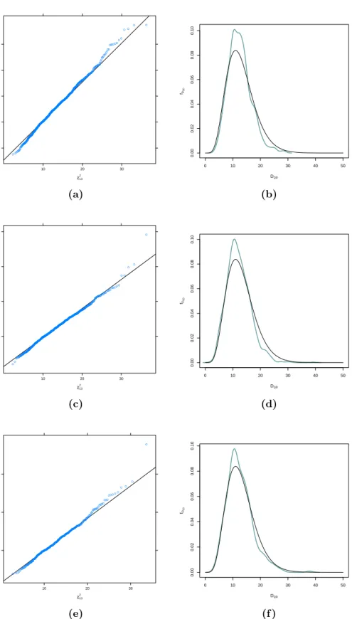
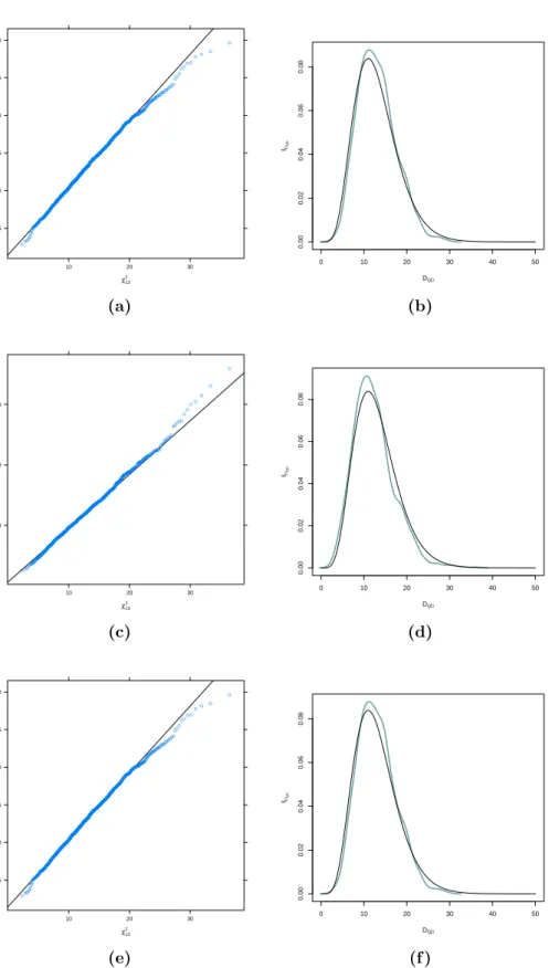
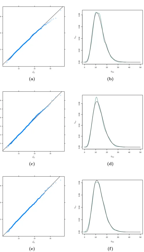
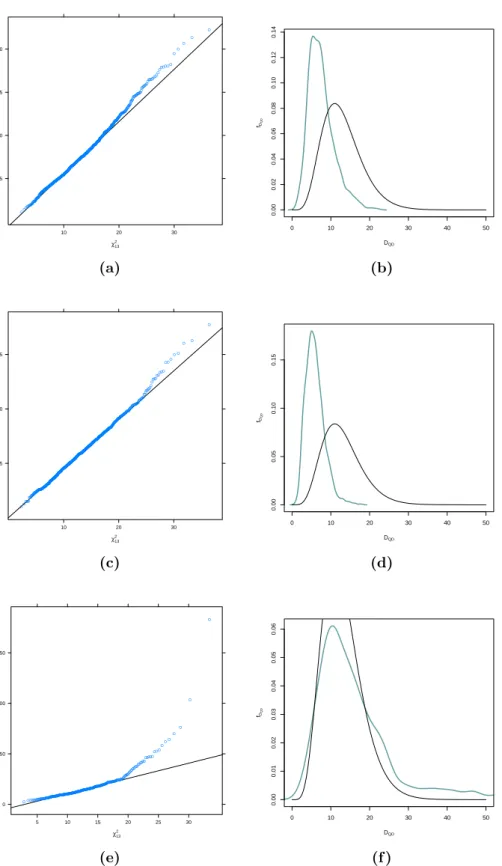
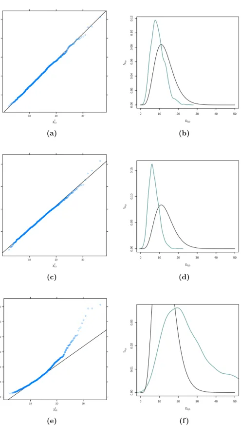
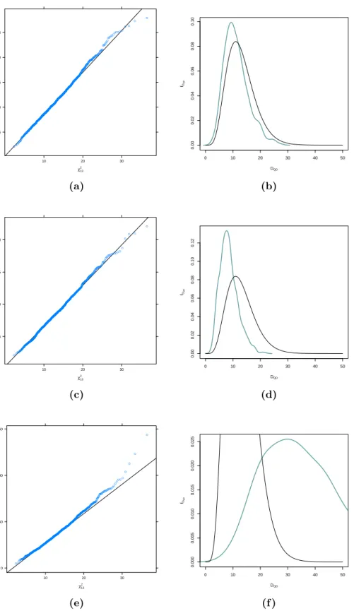
In Section4.3 we compare the sample distribution of test statistic via the maximum pseudo–likelihood estimator of copula parameters and the estima-tor provided by Kl¨uppelberg and Kuhn (2009), respectively, with the corre-sponding asymptotic distribution by QQ–plots and kernel densities. More-over, we investigate the influence of sample size and correct specification of copula on the performance of the above mentioned test statistics. Finally, we show our method at work on a financial dataset and explain differences between our copula–based and the classical normal–based approach.
Final remarks about the use of copulas in moment structure analysis and conditions in order to extend the methodology to a wider class of non–normal distributions are provided in last chapter.
Additional tools for moment structure analysis are provided in Appen-dices A and B.
Chapter 2
Inference on moment structure
models
Structural models can be defined at various levels or orders of parametric complexity. In linear structural models, common practice involves speci-fication of a structural representation for the random vector of observable variables x∈Rp; i.e.,
x=d A(ϑ0)ζ, (2.1)
whereA(ϑ0) is a matrix–valued function with respect to a vector of
popu-lation parametersϑ0. We standardly use
d
= to denote equality in distribution. The underlying generating random variables ζ ∈ Rz, for z ≥ p, may
repre-sent latent (or unobservable) variables and errors of measurement. General introduction to the field as well as more advanced treatments can be found in J¨oreskog (1978) and Browne (1982). Discussions on key developments of these topics are provided by Steiger (1994) and Bentler and Dudgeon (1996). Examples of such models include path analysis (Wright,1918,1934), prin-cipal component analysis (Hotelling, 1933; Pearson, 1901), exploratory and confirmatory factor analysis (Spearman,1904,1926), simultaneous equations (Anderson, 1976; Haavelmo, 1944), errors–in–variables models (Dolby and Freeman, 1975; Gleser, 1981), and especially the generalized linear struc-tural equations models (J¨oreskog, 1973, 1977) made popular in the social
and behavioral sciences by such computer programs as LISREL (J¨oreskog and S¨orbom, 1983) and EQS(Bentler and Wu, 1995a,b).
Statistical methods for structural models are concerned with estimating the parameters of model (2.1) in asymptotically efficient ways, as well as with testing the goodness–of–fit of (2.1). That is, the parameters of the model can be estimated, and the model null hypothesis tested, without using the
ζ variables by relying on sample estimators as ˆµ and ˆΣ of the population mean vector µ0 and covariance matrix Σ0 of the variables x, respectively.
In fact, any linear structural model implies a more basic set of parameters
θ0 = (θ0,1, . . . , θ0,q), so that µ0 =µ(θ0) and Σ0 =Σ(θ0). Theq parameters
in θ0 represent elements of ϑ0, like mean vectors, loadings, variances and
covariances or correlations of the variables ζ. Here the representation as well as the estimation and testing in model (2.1) will be restricted to a small subset of structural models, namely, those that involve continuous observable and unobservable variables whose essential characteristics can be investigated via covariance or correlation matrices.
In general, inference on covariance or correlation structure models is a straightforward matter when the model is linear and the latent variables, and hence the observed variables, are presumed to be multivariate normally tributed. Since the only unknown parameters for a multivariate normal dis-tribution are elements of mean vectors and covariance matrices, linear struc-tural model generates structures for population mean vectors and covariance matrices alone. Normal–theory–based methods such as maximum likelihood (J¨oreskog, 1967; Lawley and Maxwell, 1971) and generalized least squares (Browne,1974; J¨oreskog and Goldberger, 1972) are frequently applied. The sample mean vector and covariance matrix are jointly sufficient statistics, and maximum likelihood estimation reduces to fitting structural models to sample mean vectors and covariance matrices. Nevertheless, most social, be-havioral, and economic data are seldom normal, so normal–based methods can yield very distorted results. For example, in one distribution condition of a simulation with a confirmatory factor analysis model, Hu, Bentler, and Kano (1992) find that the likelihood ratio test based on normal–theory maxi-mum likelihood estimator rejected the true model in 1194 out of 1200 samples
11
at sample sizes that ranged from n = 150 to n = 5000. Possible deviations of the distribution function from normality have led researchers to develop asymptotically distribution free (shortly, ADF) estimation methods for co-variance structures in whichµ0 is unstructured using the minimum modified chi–squared principle by Ferguson (1958) (Browne, 1982, 1984; Chamber-lain, 1982). Although the ADF method attains reasonable asymptotically good performance on sets of few variables, in large systems with small– to medium–sized samples it can be extremely misleading; i.e., it leads to inac-curate decisions regarding the adequacy of models (Hu, Bentler, and Kano,
1992). A computationally intensive improvement on ADF statistics has been made (Yung and Bentler,1994), but the ADF theory remains inadequate to evaluate covariance structure models in such situations (Bentler and Dud-geon, 1996; Steiger, 1994).
Increasingly relaxing the normal assumption of classical moment structure analysis, one assumption still remains, namelyx∈Rp can be described as a
linear combination of some (latent) random variables ζ with existing second moments (and existing fourth moments to ensure asymptotic distributional limits of sample covariance estimators). A wider class of distributions includ-ing the multivariate normal distribution but also containinclud-ing platykurtic and leptokurtic distributions is the elliptical one. Consequently the assumption of a distribution from the elliptical class is substantially less restrictive than the usual assumption of multivariate normality. Browne (1982, 1984) intro-duces elliptical distribution theory for covariance structure analysis. Under the assumption of a distribution belonging to the elliptical class, a correction for kurtosis of normal–theory–based methods for the estimators of covariance matrix and test statistics is provided. Nevertheless, as Kano, Berkane, and Bentler (1990) point out, most empirical data have heterogeneous values of marginal kurtosis, whereas elliptical distributions require homogeneous ones. Therefore, the results based on elliptical theory may not be robust to vio-lation of ellipticity. Starting from the elliptical class, Kano, Berkane, and Bentler (1990) discuss the analysis of covariance structures in a wider class of distributions whose marginal distributions may have heterogeneous kurto-sis parameters. An attractive feature of the heterogeneous kurtokurto-sis (shortly,
HK) method is that the fourth–order moments of xdo not need to be com-puted as Browne (1984) does, because these moments are just a function of the variances and covariances between variables x and of the kurtosis pa-rameters. As a result, HK method can be used on models that are based on a substantially large number of observed variables. Unfortunately, Kano, Berkane, and Bentler (1990, Section 4) do not give necessary and sufficient conditions in order to verify the existence of elliptical distributions with dis-tinct marginal kurtosis coefficients and provide just a simple example in two dimensions.
Finally, in order to completely relax the equality in distribution assump-tion and manage flexible probability models one possible choice may be rep-resented by copulas. Nevertheless, before reviewing their use in moment structure analysis, in Section 2.1 we start with classical theoretical back-grounds concerning the estimation of θ0 in model (2.1) by weighted least
squares. The asymptotic distribution of the estimator is discussed in the ADF context and it is also considered under a more general elliptical distri-bution assumption. In Section2.2we present an example of structural model; i.e., the factor analysis model. We also talk about problems of identification and estimation whenxare assumed to be multivariate normally distributed.
2.1
Weighted least squares estimates in the
analysis of covariance structures
Let X represent a (n+ 1) ×p data matrix whose rows are drawn by a random vector of independent and identically distributed variables with population mean µ0 and population covariance matrix Σ0. A covariance
structure is a model where the elements of Σ0 are regarded as functions of a
q–dimensional parameterθ0 ∈Θ⊆Rq. ThusΣ0 is a matrix–valued function
with respect to θ0. The model is said to hold if there exists a θ0 ∈ Θ such
that Σ0 =Σ(θ0).
Let ˆΣ, the sample covariance matrix based on a sample of sizen+1, be an unbiased estimator of Σ0 and consider a discrepancy functionD
n ˆ
Σ,Σ(θ) o
WEIGHTED LEAST SQUARES ESTIMATES IN THE ANALYSIS OF COVARIANCE
STRUCTURES 13
which gives an indication of discrepancy between ˆΣ and Σ(θ) (Browne,
1982). This scalar valued function has the following properties: (P.1) D n ˆ Σ,Σ(θ) o ≥0; (P.2) D n ˆ Σ,Σ(θ) o = 0 if and only if ˆΣ=Σ(θ) (P.3) D n ˆ Σ,Σ(θ) o
is a twice continuously differentiable function of ˆΣand Σ(θ). A discrepancy functionD n ˆ Σ,Σ(θ) o
does not need to be symmetric in ˆΣ andΣ(θ), that isDnΣ,ˆ Σ(θ)odoes not need to be equal toDnΣ(θ),Σˆo. If the estimate ofθ0is obtained by minimizing some discrepancy function
DnΣ,ˆ Σ(θ)o, then DnΣ,ˆ Σˆθo= min θ∈ΘD n ˆ Σ,Σ(θ)o .
The reproduced covariance matrix will be denoted by Σˆθ = Σ
ˆ
θ
. Therefore, an estimator ˆθ, taken to minimize DnΣ,ˆ Σ(θ)o, is called a min-imum discrepancy function estimator. We call n DΣ,ˆ Σθˆ
the associated minimum discrepancy function test statistic. Since Σ0 is supposed to be
equal toΣ(θ0) according to (2.1), we shall regardθ0 as the value of θwhich
minimizes D{Σ0,Σ(θ)}; i.e.,
min
θ∈ΘD{Σ0,Σ(θ)}=D{Σ0,Σ(θ0)} .
The asymptotic distribution of the estimator ˆθ will depend on the par-ticular discrepancy function minimized. Examples of discrepancy functions are the likelihood function under the normality assumption for x,
DL n ˆ Σ,Σ(θ)o= log|Σ(θ)| −log ˆ Σ +tr h ˆ Σ{Σ(θ)}−1i−p , (2.2) which leads to the maximum likelihood estimator (J¨oreskog,1967; Lawley
and Maxwell, 1971), and the quadratic (or weighted least squares) discrep-ancy function DQD n ˆ Σ,Σ(θ) o ={σˆ −σ(θ)}>W−1{σˆ −σ(θ)} , (2.3) where σ(θ) = vech{Σ(θ)}, ˆσ =vechΣˆ, and W is a p?×p? weight
matrix converging in probability to some positive definite matrix W0 as
n → ∞, with p? = p(p+ 1)/2 (Browne, 1982, 1984). See Appendix A for
a definition of vec and vech operators. Typically W is considered to be a fixed, possible estimated, positive definite matrix, although the theory can be extended to random weight matrices (Bentler and Dijkstra, 1983). If W
is represented by 2G>p (V ⊗V)Gp, where V is a p× p positive definite
stochastic matrix which converges in probability to a positive definite matrix
V0 as n → ∞ and Gp represents the transition or duplication matrix (see
AppendixA for a formal definition), then the function in (2.3) is reduced to DGLS n ˆ Σ,Σ(θ)o= 1 2tr hn ˆ Σ−Σ(θ)oV−1i 2 , (2.4)
which is the normal–theory–based generalized least squares discrepancy function (Browne,1974; J¨oreskog and Goldberger,1972). One possible choice for V is V = ˆΣ, so that V0 = Σ0. An other possible choice for V
is V = ΣθˆM L
, where ΣθˆM L
is the estimator which maximizes the Wishart likelihood function for ˆΣ when x has a multivariate normal distri-bution (Browne, 1974).
The following usual regularity assumptions are imposed to guarantee suit-able asymptotic properties of the estimators ˆθ via quadratic discrepancy function and the associated test statistics (Browne, 1984).
(A.0) As n → ∞, n1/2 {σˆ −σ(θ
0)} converges in law to a multivariate
normal with zero mean and covariance matrix Σσ, a p? ×p? positive definite matrix.
Remark. When x is normally distributed with covariance matrix Σ0,
Σσ is represented in the form Σσ= 2G>p (Σ0⊗Σ0)Gp.
WEIGHTED LEAST SQUARES ESTIMATES IN THE ANALYSIS OF COVARIANCE
STRUCTURES 15
Remark. If x is normally distributed, (A.1) is equivalent to the con-dition that Σ0 be positive definite.
(A.2) D{Σ0,Σ(θ)}has an unique minimum on Θ atθ =θ0; i.e.,Σ(θ?) =
Σ(θ0), θ? ∈Θ, implies that θ? =θ0.
(A.3) θ0 is an interior point of the parameter space Θ.
(A.4) The p? ×q Jacobian matrix J
θ0 = J(θ0) := ∂σ(θ)/∂θ> θ=θ0 is of full rank q. (A.5) kΣ0−Σ(θ0)k isO n−1/2 .
Remark. This condition assumes that systematic errors due to lack of fit of the model to the population covariance matrix are not large relative to random sampling errors in ˆΣ. Clearly (A.5) is always satisfied if the structural model hold; i.e.,Σ0 =Σ(θ0).
(A.6) The parameter set Θ is closed and bounded.
(A.7) Jθ and, consequently,Σ(θ) are continuous function of θ.
Under the assumptions (A.0)–(A.7), Browne (1984, Corollary 2.1) and Chamberlain (1982) showed that the estimator ˆθ associated with the dis-crepancy function (2.3) is consistent and asymptotically normal and that the Cram`er–Rao lower bound of the asymptotic covariance matrix is
J>θ0Σ−σ1Jθ0
−1
, (2.5)
attained when W = Σσ. An estimator is said to be asymptotically efficient within the class of all minimum discrepancy function estimators if its asymptotic covariance matrix is equal to (2.5). In this case, the associated minimum discrepancy function test statistic, n DQD
ˆ Σ,Σˆθ
, was shown to be asymptotically chi–squared withp?−qdegrees of freedom (Browne, 1984, Corollary 4.1).
Inference based on the discrepancy function (2.3) by excluding assump-tion (A.0) is called the asymptotically distribution–free method. However,
weighted least squares estimation can easily become distribution specific. This is accomplished by specializing the optimal weight matrix W into the form that it must have if the variables have a specified distribution. In other words, the ADF method is a weighted least squares procedure in which the weight matrix has to be properly specified in order to guarantee that the asymptotic properties of standard normal theory estimators and test statis-tics are obtained. Asymptotically this method has good properties, however one needs a very large sample for the asymptotics to be appropriate (Hu, Bentler, and Kano, 1992), and sometimes it could be computationally diffi-cult to invert the p?×p? weight matrix W for moderate values of p.
When a p–variate random vectorx is elliptical distributed, the weighted least squares method can easily specialized to ellipticity. In this case, Σσ can be represented as
Σσ = 2ηG>p (Σ0⊗Σ0)Gp+G>pσ0(η−1)σ>0Gp,
whereσ0 =vec(Σ0) andη=E
n
(x−µ0)> Σ0−1 (x−µ0)o
2
/{p(p+ 2)} is the relative Mardia (1970)’s multivariate kurtosis parameter of x.
Browne (1984, Section 4) proposed a rescaled test statistic ˆ η−1n DQD ˆ Σ,Σθˆ , (2.6) where ˆ η = n+ 2 n(n+ 1) n+1 X a=1 n (xa−µˆ) > ˆ Σ−1 (xa−µˆ) o2 /{p(p+ 2)} , xa∈Rp.
Test statistic (2.6) is asymptotically chi–squared with p? −q degrees of
freedom if the structural model for covariance matrix is invariant under a constant scaling factor. This condition is satisfied if, given any θ ∈ Θ and any positive scalar c2, there exists another parameter θ? ∈
Θ such that Σ(θ?) = c2Σ(θ) (Browne, 1982, 1984). An important consequence of this adaptation is that the normal–theory–based weighted least squares method is
FACTOR ANALYSIS MODELS 17
robust against non–normality among elliptical distributions after a correction for kurtosis.
2.2
Factor analysis models
Originally developed by Spearman (1904) for the case of one common factor, and later generalized by Thurstone (1947) and others to the case of multiple factors, factor analysis is probably the most frequently used psy-chometric procedure. The analysis of moment structures originated with the factor analysis model and with some simple pattern hypothesis concerning equality of elements of mean vectors and covariance matrices. Most models involving covariance structures that are in current use are related with fac-tor analysis in some way, either by being special cases with restrictions on parameters or, more commonly, extensions incorporating additional assump-tions; see, e.g., the generalized linear structural equations models (J¨oreskog,
1973, 1977).
The aim of factor analysis is to account for the covariances of the observed variates in terms of a much smaller number of hypothetical variates or factors. The question is: if there is correlation, is there a random variateφ1 such that
all partial correlations coefficients between variables in x after eliminating the effect of φ1 are zero? If not, are there two random variates φ1 and
φ2 such that all partial correlation coefficients between variables in x after
eliminating the effects of φ1 and φ2 are zero? The process continues until
all partial correlation coefficients between variables in xare zero. Therefore, the factor analysis model partitions the covariance or correlation matrix into that which is due to common factors, and that which is unique.
To introduce the factor analysis model, let A(ϑ0) = {diag(µ),Λ,Ip}
and ζ = 1>p,φ>,υ>> in (2.1), where Ip stands for the identity matrix of
orderpand1p denotes thep–dimensional vector whose elements are all equal
to 1. The linear latent variable structure becomes
where µ ∈ Rp is a location parameter, φ ∈ Φ ⊆
Rm for m p is a vector of non–observable and uncorrelated factors and υ ∈ Υ ⊆ Rp is a
vector of noise variables υj representing sources of variation affecting only
the variate xj. Without loss of generality, we suppose that the means of all
variates are zero; i.e., E(x) = 0, E(φ) = 0, and E(υ) = 0. In the case of uncorrelated factors and of rescaled variances to unit, E φφ>
= Im.
The coefficient λj,k for k = 1, . . . , m is known as the loading of xj on φm
or, alternatively, as the loading of φm in xj. The p random variates υj are
assumed to be uncorrelated between each others and the m factors; i.e., E υυ> =Ψ = diag(ψ1, . . . , ψp) and E φυ>
= 0. The variance of υj is
termedresidual variance orunique variance of xj and denoted byψj. Then,
describing the dependence structure ofxthrough its covariance matrix yields the covariance structure,
var(x) = Σ0 =ΛΛ>+Ψ, (2.8)
namely, the dependence of xis described through the entries of Λ. Thus (2.7) corresponds to (2.1) and the parameter vector θ0 consists of
q=pm+pelements of Λ and Ψ.
2.2.1
Uniqueness of the parameters
Given a sample covariance matrix ˆΣ, we want to obtain an estimator of the parameter vector θ0. First of all, we ask whether for a specified value
of m, less than p, it is possible to define a unique Ψ with positive diagonal elements and a unique Λ satisfying (2.8). Since only arbitrary constraints will be imposed upon the parameters to define them uniquely, the model will be termedunrestricted.
Let us first suppose that there is a unique Ψ. The matrix Σ0−Ψ must
be of rankm: this quantity is equal to the covariance matrix ΛΛ> in which each diagonal element represents not the total variance of the corresponding variate inx but only the part due to the m common factors. This is known ascommunality of the variate.
UNIQUENESS OF THE PARAMETERS 19
apart from a possible change of sign of all its elements, which corresponds merely to changing the sign of the factor.
For m > 1 there is an infinity of choices for Λ. (2.7) and (2.8) are still satisfied if we replaceφbyM φandΛbyΛM>, whereM is any orthogonal matrix of order m. In the terminology of factor analysis this corresponds to a factor rotation.
Suppose that each variate is rescaled in such a way that its residual vari-ance is unity. Then
Σ?0 =Ψ−1/2Σ0Ψ−1/2 =Ψ−1/2ΛΛ>Ψ−1/2+Ip
and
Σ?0−Ip =Ψ−1/2ΛΛ>Ψ−1/2 =Ψ−1/2 (Σ0−Ψ) Ψ−1/2.
The matrixΣ?0−Ip is symmetric and of rankmand it may be expressed
in the form Ω Ξ Ω>, where Ξ is a diagonal matrix of order m, where the elements are them non zero eigenvalues ofΣ?0−Ip, andΩis ap×m matrix
satisfyingΩΩ>=Ip, where the columns are the corresponding eigenvectors.
Note thatΣ?0 has the same eigenvectors asΣ?0−Ip, and that itspeigenvalues
are those of Σ?0−Ip increased by unit.
We may define Λ uniquely as
Λ=Ψ1/2Ω Ξ1/2. (2.9) Since Ψ−1/2Λ =Ψ−1/2Ψ1/2Ω Ξ1/2 =Ω Ξ1/2, Ψ−1/2Λ > Ψ−1/2Λ=Λ>Ψ−1Λ=Ξ1/2Ω>Ω Ξ1/2 =Ξ.
Thus, from (2.9), we have chosen Λ such that Λ>Ψ−1Λ is a diagonal matrix whose positive and distinct elements are arranged in descending order of magnitude. ThenΛ and Ψare uniquely determined.
For m > 1, the fact that Λ>Ψ−1Λ should be diagonal has the effect of imposing m(m−1)/2 constraints upon the parameters. Hence the number of free (unknown) parameters in θ0 becomes
pm+p−1
2m(m−1) = q− 1
2m(m−1).
If we equate corresponding elements of the matrices on both sides of (2.8), we obtainp? distinct equations. The degrees of freedom of the model are
p?−q+1 2m(m−1) = 1 2 (p−m)2−(p+m) .
If the result of subtracting fromp? the number of free parameters is equal
to zero, we have as many equations as free parameters, so thatΛ and Ψare uniquely determined. If it is less than zero, there are fewer equations than free parameters, so that we have an infinity of choices forΛ and Ψ. Finally, if it is grater than zero, we have more equations than free parameters and the solutions are not trivial.
2.2.2
Factor Analysis by generalized least squares
We suppose that there is a uniqueΨ, with positive diagonal elements, and a uniqueΛsuch thatΛ>Ψ−1Λis a diagonal matrix whose diagonal elements are positive, distinct and arranged in decreasing order of magnitude.
Following J¨oreskog and Goldberger (1972), we assume thatxis multivari-ate normal distributed, that is ˆΣhas the Wishart distribution with expecta-tionΣ0and covariance matrix 2n−1 (Σ0⊗Σ0). Therefore, a straightforward
application of generalized least squares principle would choose parameter es-timates to minimize the quantity (2.4). Using the estimate ˆΣin place of V
in (2.4) gives DGLS n ˆ Σ,Σ(θ)o= 1 2tr n Ip −Σ(θ) ˆΣ −1o2 = 1 2tr n Ip−Σˆ −1 Σ(θ)o2 , (2.10) which is the criterion to be minimized in the generalized least squares procedure. It is also possible to show that the maximum likelihood crite-rion (2.2) can be viewed as an approximation of (2.10) under the normal distribution assumption forx.
FACTOR ANALYSIS BY GENERALIZED LEAST SQUARES 21
Equation (2.10) is now regarded as a function of Λ and Ψ and it has to be minimized with respect to these matrices. The minimization is done in two steps. We first find the conditional minimum of (2.10) for a givenΨand then we find the overall minimum.
To begin we shall assume that Ψ is nonsingular. We set equal to zero the partial derivative of (2.10) with respect to Λ and premultiplying by ˆΣ we obtain Ψ1/2Σˆ−1Ψ1/2 Ψ−1/2Λ =Ψ−1/2Λ Im+Λ>Ψ−1Λ −1 , (2.11) where we use the (ordinary) inverse of matrices of the form Ψ+ΛImΛ>
for Σ(θ). The matrix Λ>Ψ−1Λ may be assumed to be diagonal. The columns of the matrix on the right side of (2.11) then become proportional to the columns of Ψ−1/2Λ. Thus the columns of Ψ−1/2Λ are characteristic vectors of Ψ1/2Σˆ−1Ψ1/2 and the diagonal elements of Im+Λ>Ψ−1Λ
−1
are the corresponding roots. Let ξ1 ≤. . .≤ ξp be the characteristic roots of
Ψ1/2Σˆ−1Ψ1/2 and let ω1 ≤ . . . ≤ ωp be an orthonormal set of
correspond-ing characteristic vectors. Let Ξ = diag(ξ1, . . . , ξp) be partitioned as Ξ =
diag(Ξ1,Ξ2), where Ξ1 = diag(ξ1, . . . , ξm) and Ξ2 = diag(ξm+1, . . . , ξp).
LetΩ= [ω1 . . . ωp] be partitioned as Ω= [Ω1Ω2], whereΩ1 consists of the
first m vectors and Ω2 of the last p−m vectors. Then Ψ1/2Σˆ
−1
Ψ1/2 = Ω1Ξ1Ω>1 +Ω2Ξ2Ω>2 and the conditional solution ˆΛ is given by
ˆ
Λ=Ψ1/2Ω1 (Ξ1−Im)
1/2
. (2.12)
Defining ˜Σ= ˆΛΛˆ>+Ψ, it can be verified thatΨ−1/2Σ Ψ˜ −1/2 =Ω1Ξ1Ω>1+
Ω2Ω>2 and Ip−Σˆ −1 ˜ Σ=Ψ−1/2Ω2(Ip−m−Ξ2)Ω>2 Ψ 1/2 so that trIp −Σˆ −1 ˜ Σ2 =tr(Ip−m−Ξ2)2 = p X j=m+1 (ξj −1)2 .
Therefore the conditional minimum of (2.10), with respect Λfor a given Ψis the function defined by
DGLS n ˆ Σ,Σ(θ)o= 1 2 p X j=m+1 (ξj −1)2 . (2.13)
Any other set of roots will give a larger DGLS
n ˆ
Σ,Σ(θ) o
.
To start the two–steps procedure we require an initial estimate for Ψ. We could take Ψ(0)=Ip. A better choice for Ψ(0) is however given by
ˆ ψ(0)i,i = 1− 1 2m/p 1/ˆσi,i , i= 1, . . . , p , (2.14) where ˆσi,j denotes the elements in the i–th row andj–th column of ˆΣ−1. This choice has been justified by J¨oreskog (1963) and appears to work rea-sonably well in practice.
Chapter 3
Analysis of correlation
structures: the Copula
Structure Analysis
The theory for structural model analysis has been mostly developed for covariance matrices. This contrasts with common practice in which corre-lations are most often emphasized in data analysis. Correlation structures are of primary interest in situations when the different variables under con-sideration have arbitrary scales. Applying a covariance structure model to a correlation matrix will produce different test statistics, unbiased standard errors or parameter estimates and may alter the model being studied, unless the model under examination is appropriate for scale changes. The reason for this problem is not difficult to understand. If a correlation matrix is input, the elements on the main diagonal are no longer random variables: they are always equal to 1. Clearly, then, when a covariance matrix is replaced by a correlation matrix, a random vector containing p? = p(p+ 1)/2 random variables is replaced by a random vector with onlyp??=p(p−1)/2 elements
free to vary.
Scale invariance is an essential property in order to apply covariance struc-ture models to correlation matrices, but it is only minimally restrictive. The covariance structure Σ(θ) is said to be invariant under a constant scaling
factor if for any positive scalar c2 and θ ∈Θ, there exists θ? ∈
Θ such that c2Σ(θ) = Σ(θ?). The covariance structure Σ(θ) is said to be fully scale invariant if for any positive definite diagonal matrixC and anyθ ∈Θ, there exists θ? ∈ Θ such that CΣ(θ)C = Σ(θ?) (Browne, 1982). For instance, exploratory factor analysis and most of confirmatory factor analysis,LISREL, and EQS models satisfy this latter assumption. CΣ(θ)C means a change of units of measurement, therefore, if some model in multivariate analysis does not satisfy the scale invariance assumption, the model will depend on the units of measurement, which is usually unreasonable. An example of a model which is not fully scale invariant is the confirmatory factor analysis model with some factor loadings fixed at non–zero values or the confirma-tory factor analysis model with some factor loadings fixed at zero and with restrictions on factor inter–correlations (Cudeck, 1989). However, in gen-eral, by transforming a model on covariances to a model on correlations, the model will be fully scale invariant. A careful discussion of the difficulties associated with the analysis of correlation matrices as covariance matrices and related problems are provided by Cudeck (1989). Moreover, Shapiro and Browne (1990) investigate conditions under which methods intended for the analysis of covariance structures result in correct statistical conclusions when employed for the analysis of correlation structures.
Linear correlation structure analysis is concerned with the representation of the linear dependence structure aiming at a reduction in dimension. Let us consider a random vectorx∈Rpsuch that (2.1) holds. Correlation structure
analysis is now based on the assumption that the population correlation matrix of the variables,R0, satisfies the equationR0 =R(θ0), whereR(θ0)
is the correlation matrix according to the model (2.1).
Let θ0 ∈ Θ⊆ R be a q–dimensional parameter. A correlation structure model is then a matrix–valued function with respect to θ0,
R: Θ→Rp×p, θ
0 7→R(θ0) , (3.1)
such that R(θ0) is a correlation matrix.
de-COPULA THEORY: AN INTRODUCTION 25
composing the correlation structure analogously to (2.8) is justified, since dependence in normal data is uniquely determined by correlation. However, many data sets exhibit properties contradicting the normality assumption.
Copula structure analysis is a statistical method for correlation structures in-troduced by Kl¨uppelberg and Kuhn (2009) to tackle non–normality, problems of non-existing moments (second and fourth moments that ensure asymptotic distributional limits of sample covariance or correlation estimator) or differ-ent marginal distributions by using copula models. Kl¨uppelberg and Kuhn (2009) focus on elliptical copulas: as the correlation matrix is the parame-ter of an elliptical copulas, correlation structure analysis can be extended to such copulas. They only need independent and identically distributed data to ensure consistency and asymptotic normality of the estimated parameter ˆ
θ as well as the asymptotic χ2–distribution of the test statistic for model selection, that is for the estimation of the number of latent variables.
Next sections are completely devoted to briefly review the theory of cop-ulas and its use in correlation structure analysis.
3.1
Copula theory: an introduction
The history of copulas may be said to begin with Fr´echet (1951). He stud-ied the following problem, which is stated here in a bi–dimensional context: given the distribution functionsF1 andF2 of two random variablesx1 and x2
defined on the same probability space (R,B, pr), what can be said about the setC of the bivariate distribution functions whose marginals are F1 and F2?
It is immediate to note that the setC, now called the Fr´echet class of F1 and
F2, is not empty since, if x1 and x2 are independent, then the distribution
function (x1, x2)7→ F (x1, x2) =F1(x1)F2(x2) always belongs to C. But, it
was not clear which the other elements of C were. In 1959, Sklar obtained the deepest result in this respect, by introducing the notion, and the name, of copula.
Definition 3.1 For every p ≥ 2, a p–dimensional copula C is a p–variate distribution function on [0,1]p whose univariate marginals are uniformly
dis-tributed on [0,1].
Thus, each p–dimensional copula may be associated with a random vari-able u= (u1, . . . , up)
>
such that uj ∼U nif(0,1) for every j = 1, . . . , p and
u ∼ C. Conversely, any random vector whose components are uniformly distributed on [0,1] is distributed according to some copula. The notation uj ∼U nif(0,1) means that the random variable uj has uniform distribution
function on [0,1]. The notation := will be also used for representing the equality by definition later.
Sklar’s theorem is the building block of the theory of copulas; without it, the concept of copula would be one in a rich set of joint distribution functions.
Theorem 3.1 (Sklar, 1959) Let F be a p–dimensional distribution func-tion with univariate margins F1, . . . , Fp. Let Ranj denote the range of Fj,
Ranj :=Fj(R) (j = 1, . . . , p). Then, there exists a copulaC such that for all
(x1, . . . , xp)
>
∈Rp,
F (x1, . . . , xp) = C{F1(x1), . . . , Fp(xp)} . (3.2)
Such a C is uniquely determined on Ran1×. . .×Ranp and, hence, it is
unique when F1, . . . , Fp are all continuous.
Theorem 3.1 also admits the following converse implication, usually very important when one wants to construct statistical models by considering, separately, the univariate behavior of the components of a random vector and their dependence properties as captured by some copula.
Theorem 3.2 If F1, . . . , Fp are univariate distribution functions, and if C
is any p–dimensional copula, then the function F : Rp → [0,1] defined by
(3.2) is a p–dimensional distribution function with margins F1, . . . , Fp.
The joint distribution functionC of{F1(x1), . . . , Fp(xp)}
>
is then called the copula of the random vector (x1, . . . , xp)
>
or the multivariate distribution F. If F1, . . . , Fn are not all continuous it can still be shown (see Schweizer
COPULA THEORY: AN INTRODUCTION 27
and Sklar, 1983, Chapter 6) that the joint distribution function can always be expressed as in (3.2), although in this case C is no longer unique and we refer to it as a possible copula of F.
The proof of Sklar’s theorem was not given in Sklar (1959). A sketch of it was provided in Sklar (1973) (see also Schweizer and Sklar, 1974), so that for a few years practitioners in the field had to reconstruct it relying on the hand–written notes by Sklar himself. It should be also mentioned that some “indirect” proofs of Sklar’s theorem (without mentioning copula) were later discovered by Moore and Spruill (1975). More recent proofs are also provided by Sklar (1996), Burchard and Hajaiej (2006), and R¨uschendorf (2009).
Since copulas are multivariate distribution functions, they can be char-acterized in the following equivalent way.
Theorem 3.3 A function C : [0,1]p →[0,1] is a copula if, and only if, the following properties hold:
(P.1) for every j = 1, . . . , p, C(u) = uj when all the components of u are
equal to1 with the exception of the j–th one that is equal to uj ∈[0,1];
(P.2) C is isotonic; i.e., C(u)≤C(v) for all u,v ∈[0,1]p, u ≤v;
(P.3) C is p–increasing.
As a consequence, we can prove also that C(u) = 0 for every u∈[0,1]p having at least one of its components equal to 0.
Basic class of copulas are:
• the independence copula Πp(u) = u1. . . up associated with a random
vector u = (u1, . . . , up)
>
whose components are independent and uni-formly distributed on [0,1]p;
• the comonotonicity copula Mp(u) = min (u1, . . . , up) associated with a
vector u= (u1, . . . , up)
>
of random variables uniformly distributed on [0,1]p and such that u1 =. . .=up almost surely;
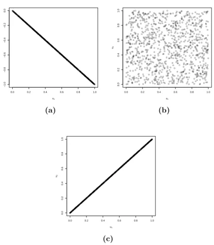
● ● ● ● ● ● ● ● ● ● ● ● ● ● ● ● ● ● ● ● ● ● ● ● ● ● ● ● ● ● ● ● ● ● ● ● ● ● ● ● ● ● ● ● ● ● ● ● ● ● ● ● ● ● ● ● ● ● ● ● ● ● ● ● ● ● ● ● ● ● ● ● ● ● ● ● ● ● ● ● ● ● ● ● ● ● ● ● ● ● ● ● ● ● ● ● ● ● ● ● ● ● ● ● ● ● ● ● ● ● ● ● ● ● ● ● ● ● ● ● ● ● ● ● ● ● ● ● ● ● ● ● ● ● ● ● ● ● ● ● ● ● ● ● ● ● ● ● ● ● ● ● ● ● ● ● ● ● ● ● ● ● ● ● ● ● ● ● ● ● ● ● ● ● ● ● ● ● ● ● ● ● ● ● ● ● ● ● ● ● ● ● ● ● ● ● ● ● ● ● ● ● ● ● ● ● ● ● ● ● ● ● ● ● ● ● ● ● ● ● ● ● ● ● ● ● ● ●● ● ● ● ● ● ● ● ● ● ● ● ● ● ● ●● ● ● ● ● ● ● ● ● ● ● ● ● ● ● ● ● ● ● ● ● ● ● ● ● ● ● ● ● ● ● ● ●● ● ● ● ● ● ● ● ● ● ● ● ● ● ● ● ● ● ● ● ● ● ● ● ● ● ● ● ● ● ● ● ● ● ● ● ● ● ● ● ● ● ● ● ● ● ● ● ● ● ● ● ● ● ● ● ● ● ● ● ● ● ● ● ●● ● ● ● ● ● ● ● ● ● ● ● ● ● ● ● ● ● ● ● ● ● ● ● ● ● ● ● ● ● ● ● ● ● ● ● ● ● ● ● ● ● ● ● ● ● ● ● ● ● ● ● ● ● ● ● ● ● ● ● ● ● ● ● ● ● ● ● ● ● ● ● ● ● ● ● ● ● ● ● ● ● ● ● ● ● ● ● ● ● ● ● ● ● ● ● ● ● ● ● ● ●● ● ● ● ● ● ● ● ● ● ● ● ● ● ● ● ● ● ● ● ● ● ● ● ● ● ● ● ● ● ● ● ● ● ● ● ● ● ● ●● ● ● ● ● ● ● ● ● ● ● ● ● ● ● ● ● ● ● ● ● ● ● ● ● ● ● ● ● ● ● ● ● ● ● ● ● ● ● ● ● ● ● ● ● ● ● ● ● ● ● ● ● ● ● ● ●● ● ● ● ● ● ● ● ● ● ● ● ● ● ● ● ● ● ● ● ● ● ● ● ● ● ● ● ● ● ● ● ● ● ● ● ● ● ● ● ● ● ● ● ● ● ● ● ● ● ● ● ●● ● ● ● ● ● ● ● ● ● ● ● ● ● ● ● ● ●● ● ● ● ● ● ● ● ● ● ● ● ● ● ● ● ● ● ● ● ● ● ● ● ● ● ● ● ● ● ● ● ● ● ● ● ● ● ● ● ● ● ● ● ● ● ● ● ● ● ● ● ● ● ● ● ● ● ● ● ● ● ● ● ● ● ● ● ● ● ● ● ● ● ● ● ● ● ● ● ● ● ● ● ● ● ● ● ● ● ● ● ● ● ● ● ● ● ● ● ● ● ● ● ●● ● ● ● ● ● ● ● ● ● ● ● ● ● ● ● ● ● ● ● ● ● ● ● ● ● ● ● ● ● ● ● ● ● ● ● ● ● ● ● ● ● ● ● ● ●● ● ● ● ● ● ● ● ● ● ● ● ● ● ● ● ● ● ● ● ● ● ● ● ● ● ● ● ● ● ● ● ● ● ● ● ● ● ● ● ● ● ● ● ● ● ● ● ● ● ● ● ● ● ● ● ● ● ● ● ● ● ● ● ● ● ● ● ● ● ● ● ● ● ● ● ● ● ● ● ● ● ● ● ● ● ● ● ● ● ● ● ● ● ● ● ● ● ● ● ● ● ● ● ● ● ● ● ● ● ● ● ● ● ● ● ● ● ● ● ● ● ● ● ● ● ● ● ● ● ● ● ● ● ● ● ● ● ● ● ● ● ● ● ● ● ● ● ● ● ● ● ● ● ● ● ● ● ● ● ● ● ● ● ● ● ● ● ● ● ● ● ● ● ● ● ● ● ● ● ● ● ● ● ● ● ● ● ● ● ● ● ● ● ● ● ● ● ● ● ● ● ● ● ● ● ● ● ● ● ● ● ● ● ● ● ● ● ● ● ● ● ● ● ● ● ● ● ● ● ● ● ● ● ● ● ● 0.0 0.2 0.4 0.6 0.8 1.0 −1.0 −0.8 −0.6 −0.4 −0.2 0.0 u1 u2 (a) ● ● ● ● ● ● ● ● ● ● ● ● ● ● ● ● ● ● ● ● ● ● ● ● ● ● ● ● ● ● ● ● ● ● ● ● ● ● ● ● ● ● ● ● ● ● ● ● ● ● ● ● ● ● ● ● ● ● ● ● ● ● ● ● ● ● ● ● ● ● ● ● ● ● ● ● ● ● ● ● ● ● ● ● ● ● ● ● ● ● ● ● ● ● ● ● ● ● ● ● ● ● ● ● ● ● ● ● ● ● ● ● ● ● ● ● ● ● ● ● ● ● ● ● ● ● ● ● ● ● ● ● ● ● ● ● ● ● ● ● ● ● ● ● ● ● ● ● ● ● ● ● ● ● ● ● ● ● ● ● ● ● ● ● ● ● ● ● ● ● ● ● ● ● ● ● ● ● ● ● ● ● ● ● ● ● ● ● ● ● ● ● ● ● ● ● ● ● ● ● ● ● ● ● ● ● ● ● ● ● ● ● ● ● ● ● ● ● ● ● ● ● ● ● ● ● ● ● ● ● ● ● ● ● ● ● ● ● ● ● ● ● ● ● ● ● ● ● ● ● ● ● ● ● ● ● ● ● ● ● ● ● ● ● ● ● ● ● ● ● ● ● ● ● ● ● ● ● ● ● ● ● ● ● ● ● ● ● ● ● ● ● ● ● ● ● ● ● ● ● ● ● ● ● ● ● ● ● ● ● ● ● ● ● ● ● ● ● ● ● ● ● ● ● ● ● ● ● ● ● ● ● ● ● ● ● ● ● ● ● ● ● ● ● ● ● ● ● ● ● ● ● ● ● ● ● ● ● ● ● ● ● ● ● ● ● ● ● ● ● ● ● ● ● ● ● ● ● ● ● ● ● ● ● ● ● ● ● ● ● ● ● ● ● ● ● ● ● ● ● ● ● ● ● ● ● ● ● ● ● ● ● ● ● ● ● ● ● ● ● ● ● ● ● ● ● ● ● ● ● ● ● ● ● ● ● ● ● ● ● ● ● ● ● ● ● ● ● ● ● ● ● ● ● ● ● ● ● ● ● ● ● ● ● ● ● ● ● ● ● ● ● ● ● ● ● ● ● ● ● ● ● ● ● ● ● ● ● ● ● ● ● ● ● ● ● ● ● ● ● ● ● ● ● ● ● ● ● ● ● ● ● ● ● ● ● ● ● ● ● ● ● ● ● ● ● ● ● ● ● ● ● ● ● ● ● ● ● ● ● ● ● ● ● ● ● ● ● ● ● ● ● ● ● ● ● ● ● ● ● ● ● ● ● ● ● ● ● ● ● ● ● ● ● ● ● ● ● ● ● ● ● ● ● ● ● ● ● ● ● ● ● ● ● ● ● ● ● ● ● ● ● ● ● ● ● ● ● ● ● ● ● ● ● ● ● ● ● ● ● ● ● ● ● ● ● ● ● ● ● ● ● ● ● ● ● ● ● ● ● ● ● ● ● ● ● ● ● ● ● ● ● ● ● ● ● ● ● ● ● ● ● ● ● ● ● ● ● ● ● ● ● ● ● ● ● ● ● ● ● ● ● ● ● ● ● ● ● ● ● ● ● ● ● ● ● ● ● ● ● ● ● ● ● ● ● ● ● ● ● ● ● ● ● ● ● ● ● ● ● ● ● ● ● ● ● ● ● ● ● ● ● ● ● ● ● ● ● ● ● ● ● ● ● ● ● ● ● ● ● ● ● ● ● ● ● ● ● ● ● ● ● ● ● ● ● ● ● ● ● ● ● ● ● ● ● ● ● ● ● ● ● ● ● ● ● ● ● ● ● ● ● ● ● ● ● ● ● ● ● ● ● ● ● ● ● ● ● ● ● ● ● ● ● ● ● ● ● ● ● ● ● ● ● ● ● ● ● ● ● ● ● ● ● ● ● ● ● ● ● ● ● ● ● ● ● ● ● ● ● ● ● ● ● ● ● ● ● ● ● ● ● ● ● ● ● ● ● ● ● ● ● ● ● ● ● ● ● ● ● ● ● ● ● ● ● ● ● ● ● ● ● ● ● ● ● ● ● ● ● ● ● ● ● ● ● ● ● ● ● ● ● ● ● ● ● ● ● ● ● ● ● ● ● ● ● ● ● ● ● ● ● ● ● ● ● ● ● ● ● ● ● ● ● ● ● ● ● ● ● ● ● ● ● ● ● ● ● ● ● ● ● ● ● ● ● ● ● ● ● ● ● ● ● ● ● ● ● ● ● ● ● ● ● ● ● ● ● ● ● ● ● ● ● ● ● ● ● ● ● 0.0 0.2 0.4 0.6 0.8 1.0 0.0 0.2 0.4 0.6 0.8 1.0 u1 u2 (b) ● ● ● ● ● ● ● ● ● ● ● ● ● ● ● ● ● ● ● ● ● ● ● ● ● ● ● ● ● ● ● ● ● ● ● ● ● ● ● ● ● ● ●● ● ● ●● ● ● ● ● ● ● ● ● ● ● ● ● ● ● ● ● ● ● ● ● ● ● ● ● ● ● ● ● ●● ● ●● ● ● ● ● ● ● ● ● ● ● ● ● ● ● ● ● ● ● ● ● ● ● ● ● ● ● ● ● ● ● ● ● ● ● ● ● ● ● ● ● ● ● ● ● ● ● ● ● ● ● ● ● ● ● ● ● ● ● ● ● ● ● ● ● ● ● ● ● ● ● ● ● ● ● ● ● ● ● ● ● ● ● ● ●● ●● ● ● ● ● ● ● ● ● ● ● ● ● ● ● ● ● ● ● ● ● ● ● ● ● ● ● ● ● ● ● ● ● ● ● ● ● ● ● ● ● ● ● ● ● ● ● ● ● ● ● ● ● ● ● ● ● ● ● ● ● ● ● ● ● ● ● ● ● ● ● ● ● ● ● ● ● ● ● ● ● ● ● ● ● ● ● ● ●● ● ● ● ● ● ● ● ● ● ● ● ● ● ● ● ● ● ● ● ● ● ● ● ● ● ● ● ● ● ● ● ● ● ● ● ● ● ● ● ● ● ● ● ● ● ● ● ● ● ● ● ● ● ● ● ● ● ● ● ● ● ● ● ● ● ● ● ● ● ● ● ● ● ● ● ● ● ● ● ●●● ● ● ● ● ● ● ● ● ● ● ● ● ● ● ● ● ● ● ● ● ● ● ● ● ● ● ● ● ● ● ●● ● ● ●● ● ● ● ● ● ● ● ● ● ● ● ● ● ● ●● ● ● ● ● ● ● ● ● ● ● ● ● ● ● ● ● ● ● ● ● ● ● ● ● ● ● ● ● ● ● ● ● ● ● ● ● ● ● ● ● ● ● ● ● ● ● ● ● ● ● ● ● ● ● ● ● ● ● ● ● ● ● ● ● ● ● ● ● ● ● ● ● ● ● ● ● ● ● ● ● ● ● ● ● ● ● ● ●● ● ● ● ● ● ● ● ● ● ● ● ● ● ● ● ● ● ● ● ● ● ● ● ● ● ● ● ● ● ● ● ● ● ● ● ● ● ● ● ● ● ● ● ● ● ● ● ● ● ● ● ● ● ● ● ● ● ● ● ● ● ● ● ● ● ● ● ● ● ● ● ● ●● ● ● ● ● ● ● ● ● ● ● ● ● ● ● ● ● ● ● ● ● ● ● ● ● ● ● ● ● ● ● ● ● ● ● ● ● ● ● ● ● ● ● ● ● ● ● ● ● ● ● ● ● ● ● ● ● ● ● ● ● ● ● ● ● ● ● ● ● ● ● ● ● ● ● ● ● ● ● ● ● ● ● ● ● ● ● ● ● ● ● ● ● ● ● ● ● ● ● ● ● ● ● ● ● ● ● ● ● ● ● ● ● ● ● ● ● ● ● ● ● ● ● ● ● ● ● ● ● ● ● ● ● ● ● ● ● ● ● ● ● ● ● ● ● ● ● ● ● ● ● ● ● ● ● ● ● ● ● ● ● ● ● ● ● ● ● ● ● ● ● ● ● ● ● ● ● ● ● ● ● ● ● ● ● ● ● ● ● ● ● ● ● ● ● ● ● ● ● ● ● ● ● ● ● ●● ● ● ● ● ● ● ● ● ● ● ● ● ● ● ● ● ● ● ● ● ● ● ● ● ● ● ● ● ● ● ● ● ● ● ● ● ● ● ● ● ● ● ● ● ● ● ● ● ● ● ● ● ● ● ● ●● ● ● ● ● ● ● ● ● ● ● ● ● ● ● ● ● ● ● ● ● ● ● ● ● ● ● ● ● ● ● ● ● ● ● ● ● ● ● ● ● ● ● ● ● ● ● ● ● ● ● ● ● ● ● ● ● ● ● ● ● ● ● ● ● ● ● ● ● ● ● ● ● ● ● ● ● ● ● ● ● ● ● ● ● ● ● ● ● ● ● ● ● ● ● ● ● ● ● ● ● ● ● ● ● ● ● ● ● ● ● ● ● ● ● ● ● ● ● ● ● ● ● ● ● ● ● ● ● ● ● ● ● ● ● ● ●● ● ● ● ● ● ● ● ● ● ● ● ● ● ● ●●● ●● ● ● ● ● ● ● ● ● ● ● ● ● ● ● ● ● ● ● ● ● ● ● ● ● ● ● ● 0.0 0.2 0.4 0.6 0.8 1.0 0.0 0.2 0.4 0.6 0.8 1.0 u1 u 2 (c)
Figure 3.1: Independent realizations from bivariate countermonotonicity (a), indepen-dence (b), comonotonicity (c) copulas, respectively.
• the countermonotonicity copula W2(u1, u2) = max{u1+u2−1,0}
as-sociated with a vector u = (u1, u2)
>
of random variables uniformly distributed on [0,1]2 and such that u1 = 1−u2 almost surely.
By summarizing, from any p–variate distribution function F one can derive a copula C via (3.2). Specifically, when Fj is continuous for every
j = 1, . . . , p,C can be obtained by means of the formula C(u1, . . . , up) =F
F1−1(u1), . . . , Fp−1(up) ,
where Fj−1(u) := inf{x∈R|Fj(x)≥u , u∈[0,1]} denotes the pseudo–
COPULA THEORY: AN INTRODUCTION 29
random variables (x1, . . . , xp)
>
into another random variable (u1, . . . , up)
>
, uj =Fj(xj), having the margins uniform on [0,1] and preserving the
depen-dence among the components. Alternatively, one could transform x to any other distribution, but U nif(0,1) is particularly easy.
On the other hand, any copula can be combined with different univariate distribution functions in order to obtain ap–variate distribution function by using (3.2). In particular, copulas can serve for modeling situations where a different distribution is needed for each marginal, providing a valid alter-native to several classical multivariate distribution functions such Gaussian, Student’s t, Pareto, etc., as Durante and Sempi (2010) point out.
In what follows, we deal with semi–parametric copula models P, which are defined as follows. Let C = Cx(·; α) :α∈A⊂Rd be a parametric family of copulas on [0,1]p with density cx(·; α) with respect to Lebesgue measure on [0,1]p, indexed by a d–dimensional real parameter vector α.
For α ∈ A and arbitrary distribution functions F1, . . . , Fp on R, let
Fα,F1,...,Fp be the distribution function on R
p defined by
Fα,F1,...,Fp(x1, . . . , xp) =Cx{F1(x1), . . . , Fp(xp) ;α}
for (x1, . . . , xp) ∈ Rp. Then with pr(·;α, F1, . . . , Fp) denoting the
cor-responding probability measure on (Rp,Bp), where Rp is the p–dimensional real Euclidean space andBp its Borelσ–field, andF denoting the collection
of all distribution function on R,
P ={pr(·;α, F1, . . . , Fp) :α∈A, Fj ∈F, j = 1, . . . , p}
is a semi–parametric copula model.
One simple example, which is widely exploited by Kl¨uppelberg and Kuhn (2009), is provided by the family of elliptical copulas being the copulas of elliptical distributions. These copulas are very flexible and easy to handle also in high dimensions. For instance, let us consider the copula resulting from the multivariate normal distribution onRp,F
µ0,Σ0, having mean vector
µ0 and covariance matrix Σ0. Let Fj denote the one–dimensional standard
Cx(u1, . . . , up;α) =Fx
F1−1(u1), . . . , Fp−1(up) ; α
where, in this case, α consists of the population linear correlation coeffi-cients between variables x.
3.1.1
The elliptical and meta–elliptical copulas
As underlined in the previous section, copulas play an important role in the construction of multivariate distribution function. As a consequence, having at one’s disposal a variety of copulas can be very useful for build-ing stochastic models with different properties, sometimes indispensable in practice (e.g., heavy tails, asymmetries, etc.). Therefore, several investiga-tions have been carried out concerning the construction of different families of copulas and their properties. In this work we deal just two of them, by focusing in this chapter on the family that Kl¨uppelberg and Kuhn (2009) use in their work, namely, elliptical copulas. Different families (or construction methods) are discussed in the books of Joe (1997) and Nelsen (2006).
Elliptical copulas describe the dependence structure in elliptical distribu-tions as well as in their extensions, the meta–elliptical distribudistribu-tions, which have been originally introduced in Fang, Fang, and Kotz (2002). Their prop-erties are examined by Frahm, Junker, and Szimayer (2003) and Abdous, Genest, and R`emillard (2005). These dependence structures are popular in actuarial science and in finance; see Malevergne and Sornette (2003), Cheru-bini, Luciano, and Vecchiato (2004), McNeil, Frey, and Embrechts (2005) and references therein. We start by recalling the definition of an elliptical distribution and we refer to Fang, Kotz, and Ng (1990) for a comprehensive overview.
A random vector x ∈ Rp has an elliptical distribution with parameters
µ0 ∈ Rp and a positive (semi) definite matrix Σ
0 ∈ Rp×p, if x has the
stochastic representation