Title
Improving Precipitation Estimation Using Convolutional Neural Network
Permalink
https://escholarship.org/uc/item/8nb145xd
Journal
WATER RESOURCES RESEARCH, 55(3)
ISSN
0043-1397
Authors
Pan, Baoxiang
Hsu, Kuolin
AghaKouchak, Amir
et al.
Publication Date
2019-03-01
DOI
10.1029/2018WR024090
License
https://creativecommons.org/licenses/by/4.0/ 4.0
Peer reviewed
Baoxiang Pan1 , Kuolin Hsu1, Amir AghaKouchak1,2 , and Soroosh Sorooshian1,2
1Center for Hydrometeorology and Remote Sensing, University of California, Irvine, CA, USA,2Department of Earth
System Science, University of California, Irvine, CA, USA
Abstract
Precipitation process is generally considered to be poorly represented in numericalweather/climate models. Statistical downscaling (SD) methods, which relate precipitation with model resolved dynamics, often provide more accurate precipitation estimates compared to model's raw precipitation products. We introduce the convolutional neural network model to foster this aspect of SD for daily precipitation prediction. Specifically, we restrict the predictors to the variables that are directly resolved by discretizing the atmospheric dynamics equations. In this sense, our model works as an alternative to the existing precipitation-related parameterization schemes for numerical precipitation estimation. We train the model to learn precipitation-related dynamical features from the surrounding dynamical fields by optimizing a hierarchical set of spatial convolution kernels. We test the model at 14 geogrid points across the contiguous United States. Results show that provided with enough data, precipitation estimates from the convolutional neural network model outperform the reanalysis precipitation products, as well as SD products using linear regression, nearest neighbor, random forest, or fully connected deep neural network. Evaluation for the test set suggests that the improvements can be seamlessly transferred to numerical weather modeling for improving precipitation prediction. Based on the default network, we examine the impact of the network architectures on model performance. Also, we offer simple visualization and analyzing approaches to interpret the models and their results. Our study contributes to the following two aspects: First, we offer a novel approach to enhance numerical precipitation estimation; second, the proposed model provides important implications for improving precipitation-related parameterization schemes using a data-driven approach.
Plain Language Summary
The precipitation process is not well simulated in numericalweather models, since it takes place at the scales beyond the resolution of current models. We develop a statistical model using deep learning technique to improve the estimation of precipitation in numerical weather models.
1. Introduction
The modeling of the atmosphere is typically based on a particular set of partial differential equations, which is derived by applying the conservation laws and thermodynamic laws on the continuous “control volume” of the atmosphere (Bjerknes, 1906; Holton & Hakim, 2012). With the rapid growth of computing power, we can discretize and resolve these equations on increasingly finer computing grids. However, there remains many critical subgrid scale processes that are not explicitly resolved.
A well-concerned example is the precipitation process. Precipitation estimation involves explicit and implicit representations of the cloud physics, such as the water vapor convection, phase change, and particle coa-lescence. These processes take place at millimeter to molecule scales, which far surpass the resolution of current numerical models (O(1km)∕O(10km) −O(100km)for weather/climate models). Also, the assump-tions of thermodynamic equilibrium and continuity lose their validity in describing some of the microscopic processes (Stensrud, 2009), making it necessary to adopt supplementary equations for physically solid simulations.
In numerical models, such unresolved processes are inferred from the resolved dynamics on the computa-tional grid (Kalnay, 2003). This process is known as parameterization. Specific to precipitation, the directly related parameterization schemes are cloud microphysics and subgrid convection. Given the intrinsic
Special Section:
Big Data & Machine Learning in Water Sciences: Recent Progress and Their Use in Advancing Science
Key Points:
• We offer a novel approach to enhance numerical precipitation estimation using deep convolutional neural network (CNN)
• The model provides important implications for improving precipitation-related parameterization schemes using a data-driven approach • The CNN model outperforms existing precipitation statistical downscaling approaches by learning dominant spatial dynamics features
Supporting Information: • Supporting Information S1 Correspondence to: B. Pan, [email protected] Citation:
Pan, B., Hsu, K., AghaKouchak, A., & Sorooshian, S. (2019). Improving precipitation estimation using convolutional neural network.Water Resources Research,55, 2301–2321. https://doi.org/10.1029/2018WR024090
Received 19 SEP 2018 Accepted 9 JAN 2019
Accepted article online 15 JAN 2019 Published online 22 MAR 2019
©2019. American Geophysical Union. All Rights Reserved.
complexity of the cloud and precipitation process, the equations and their associated parameters in these parameterization schemes are generally of high structural and parametric uncertainties (Draper, 1995). As a result, models' precipitation products are usually considered less reliable compared to the directly resolved variables, such as pressure and temperature (Betts et al., 1998; Bukovsky & Karoly, 2007; Higgins et al., 1996; Tian et al., 2017; Vitart, 2004).
Statistical downscaling (SD) methods are also used for the purpose of inferring the poorly represented pro-cesses from the resolved dynamics and other data sources. However, SD has distinct objectives compared to the parameterization schemes. The main purpose of parameterization is to depict the subgrid scale pro-cesses for realistic atmosphere modeling. The primary concern for SD, as indicated by the name, is to resolve the scale discrepancy between the existing model simulations and application requirements (Maraun et al., 2010). Accordingly, the model input/output, resolution, usage, and complexity of parameterization schemes and SD are different.
Besides the scaling issue, another aspect of SD is noted in practices: Compared to raw outputs or the dynamically downscaled outputs from numerical models, SD occasionally provides more accurate estimates of the unresolved processes. This is because SD is customized for specific objective, region, and climate condition. The data-driven model with carefully designed model architecture and calibrated parameters may outperform the default parameterization schemes in relating the unresolved processes to resolved circulation. This phenomenon offers valuable implications for improving the relevant parameterization schemes and opportunities for enhancing the prediction of the parameterized processes (Rasp et al., 2018; Schneider et al., 2017).
Here we focus on fostering this aspect of SD for weather-scale precipitation forecast. Specifically, we propose to improve the accuracy of daily precipitation estimates through relating the precipitation process with the circulation data that are explicitly resolved in the atmospheric primitive equations. Compared to conven-tional SD applications, the task here poses much higher requirements on model resolution and accuracy. Recent developments in machine learning (ML) techniques, especially the branch of deep neural networks (DNNs), offer an opportunity for describing and predicting such complicated physical processes using a compose of big data and advanced model architectures. Here we illustrate how a particular form of DNN, named convolutional neural network (CNN; LeCun et al., 1998), can be adapted to address the precipitation estimation problem.
The rest of the paper is organized as follows: We start with a brief review of relevant works. Then, we formulate the problem and illustrate the model requirements for this application.
The model is described and tested thereafter. We show the model results and provide methods for analyz-ing and interpretanalyz-ing the models. We compare the model performance with some of the widely adopted SD approaches. Conclusions are drawn at last.
2. Related Works
Many studies have been conducted on improving precipitation prediction accuracy with statistical approaches. We review the relevant SD methods, for which the objective and methodology are closely related to our work here. Also, we briefly review the basic concepts of DNNs, with a special emphasis on their applications in physical processes.
2.1. Statistical Downscaling
Following the survey in Maraun et al. (2010), SD approaches are classified into perfect prognosis (PP), model output statistics (MOS), and weather generators. Since the objective for our study is deterministic precipitation prediction, we focus on SD approaches that make deterministic estimates of precipitation or its estimation biases. This includes PP and MOS. The weather generator models are not reviewed here. PP models construct statistical relations between the large-scale predictors and local scale predictands (Fowler et al., 2007; Maraun et al., 2010). Both the predictors and predictands are considered to be realisti-cally simulated or observed, hence the name of “perfect.” Along with the advancement of general circulation models (GCMs), many precipitation PP methods have been developed. The simplest form is linear regres-sion, which estimates precipitation using an optimized linear combination of the local circulation features (Hannachi et al., 2007; Jeong et al., 2012; Li & Smith, 2009; Murphy, 2000). The predictors usually consist of
the raw variables or the leading principal components (PCs) of the moisture, pressure, and wind field (Wilby & Wigley, 2000). Besides the linear models, there are also approaches that utilize the nonlinear features of relevant circulation field, such as self-organizing map (Hope, 2006), support vector machine (Tripathi et al., 2006), nearest neighbor (Gangopadhyay et al., 2005), random forest (Hutengs & Vohland, 2016), and artificial neural network (ANN; Schoof & Pryor, 2001).
MOS stands for the practice of using statistical approaches to enhance the model's prediction accuracy (Glahn & Lowry, 1972). Compared to PP, MOS is more frequently used in regional circulation models (RCMs) than in GCMs (Maraun et al., 2010). Also, the predictors of MOS are numerical models' raw outputs, which are not assumed to be perfectly estimated. For instance, a typical application of MOS is to correct the biases of the numerical model's raw precipitation estimates (Jakob Themeßl et al., 2011). It should be noted that the validity and universality of precipitation MOS rely on the consistency of precipitation estimation biases, which is usually not guaranteed, given the continuous improvements of numerical models.
The performances of the above-mentioned SD approaches have been compared with dynamical downscaling results (Ayar et al., 2016; Gutmann et al., 2012; Haylock et al., 2006; Murphy, 1999; Schmidli et al., 2007; Tang et al., 2016). For instance, an intercomparison of six SD models and five RCMs for Europe indicated that PP and MOS models achieved higher skill scores in estimating certain aspects of precipitation, such as the occurrence and intensity (Ayar et al., 2016). On the other hand, another comparison study showed clear advantage of RCMs for estimating precipitation over complex terrain (Schmidli et al., 2007). Overall, the performance of SD depends on many factors, including the selection of predictors, the model and its implementation, the available data, and the climate condition.
2.2. DNNs and Their Applications for Physical Processes
DNNs belong to the domain of ML, which covers a general scope of computer-aided statistical modeling. DNNs differ from traditional ML approaches in their modeling workflow. In a canonical ML modeling pro-cess, the raw form data, which quantify certain attributes of the study object, should be transformed into a suitable feature vector before being effectively processed for the learning objective (Goodfellow et al., 2016; LeCun et al., 2015). The feature extraction process is typically performed in separation with the modeling process. Despite the expert knowledge and engineering works required for the feature extraction process, a predefined feature extractor captures little useful information beyond our prior knowledge. This issue is particularly severe for high-dimensional problems, where it is difficult to have foresight in the intricate but important data structures.
On the other hand, DNNs, together with a broader family of representation learning approaches (Bengio et al., 2013), offer an “end-to-end” modeling workflow: The feature extraction process is integrated into the modeling process, which allows the model to learn customized features rather than subject to the pre-engineered features.
DNNs learn to customize features through building multiple levels of representation of the data, which are achieved by composing simple but nonlinear modules (named as neurons) that each transform the repre-sentation at one level into a reprerepre-sentation at a higher, slightly more abstract level (LeCun et al., 2015). The differentiability of the hierarchical model allows applying the gradient descent algorithm to tune the neurons' parameters in order to make the model exhibit desired behavior. This process is widely known as backpropagation training (Rumelhart et al., 1985; Werbos, 1982). In addition to these basic concepts, mod-ern DNNs involve numerous network architecture variations, training algorithms and tricks, regularization methods, among others. A comprehensive review is beyond the scope of this work and can be found in LeCun et al. (2015), Schmidhuber (2015), and Goodfellow et al. (2016). A transdisciplinary review of DNN relevant to water resources-related research can be found in Shen (2018) and Shen et al. (2018).
DNNs have dramatically improved the state of the art in applications that cannot be adequately solved with a deterministic rule-based solution, such as visual recognition (Krizhevsky et al., 2012), speech recognition (Amodei et al., 2016), video prediction (Lotter et al., 2016), and natural language processing (Socher et al., 2011). For the modeling of the natural physical processes, where we have established principled solutions through analytic descriptions of the scientist's prior knowledge of the underlying processes (de Bezenac et al., 2017), dynamical simulations are preferred to ML-based approaches. However, recent developments showed that provided with (1) big amount of data and (2) well-designed network architectures that encode
Figure 1.(a) The case study area of a32km×32km geogrid centered at46◦N,122◦W. Its surrounding circulation field is delineated with the800km×800km red polygon. (b) The geogrid's daily precipitation time series from 1979 to 2017. The red thick line represents the gage-based precipitation records from the National Oceanic and Atmospheric Administration Climate Prediction Center (CPC); the blue slim line represents the model reanalysis records from the National Centers for Environmental Prediction North American Regional Reanalysis Project (NARR). Data details are given in the section 5.1. (c) The every 3-hr snapshots of the circulation profile for the storm event that happened on 7 November 2006. The geopotential height (GPH) at 1,000, 850, and 500 hPa and the total column precipitable water are obtained form NARR. Data are normalized by subtracting the field mean (𝜇) and dividing by the field standard deviation (𝜎).
the physical background knowledge, DNNs are competitive with numerical methods in simulating complex natural processes.
Generally, two motivations are found for adopting a data-driven model besides the classical dynamical simulation. The first is computing efficiency. The computational demanding components in numerical sim-ulations can be replaced by data-driven model counterparts to accelerate the simulation without significant loss of accuracy. Examples include using DNNs to simulate the Eulerian fluid (Tompson et al., 2016) and to predict the pressure field evolution in fluid flow (Wiewel et al., 2018). The other concern is to repre-sent the unresolved processes beyond the original numerical simulation. For instance, Gentine et al. (2018) trained a neural network to represent the subgrid scale convection process in atmospheric modeling. The trained model was coupled in GCMs and skillfully predicted many of the convective heating, moistening, and radiative features. Xie et al. (2018) applied a a conditional generative adversarial network to generate spatiotemporal coherent high-resolution fluid flow based on its low-resolution estimates.
For the applications mentioned above, a particular DNN architecture named CNN acts as a core building block. Compared to conventional neural networks, CNNs have significantly enhanced our capacity in pro-cessing structured high-dimensional data. This is achieved by utilizing the inner structure of the data to reduce the model structural redundancy and foster effective information extraction. Geophysical data are intrinsically structured in space and time. The huge geophysical data sets from remote sensing observations, numerical simulations, and their composite offer precious deposits for the application of DNNs (Tao et al., 2016). CNNs have found applications in detecting extreme weather from the climate data sets (Liu et al., 2016) and precipitation nowcasting (Shi et al., 2017; Xingjian et al., 2015). More related to our objective, Vandal et al. (2017) developed a super-resolution convolutional neural network for precipitation SD. The low-resolution precipitation field (1◦) and elevation field data were fed into the super-resolution convolu-tional neural network to produce the high-resolution precipitation field (1
8
◦
). We noted that many of these geophysical CNN applications took little use of the atmospheric dynamical modeling products, which offer physically solid and comprehensive information of the atmosphere. While many recent research works have started to explore the applicability of DNN for parameterizing the unresolved processes in fluid and geofluid modeling (Ling et al., 2016; Rasp et al., 2018), it remains a question how DNN can translate the big data of observations and numerical simulations into precipitation estimation improvements (Pan et al., 2017).
3. Problem Formulation
To formulate the precipitation estimation problem, we first clarify the context by introducing a real-world precipitation scenario. Figure 1 shows a winter storm that hit the windward slope of the Cascade Range between Washington State and Oregon State of the United States. The case is selected for two reasons. First, we have well-developed conceptual and theoretical models for describing such extratropical winter pre-cipitation processes (Bjerknes, 1951; Rossby, 1939). The well-established models offer accessible concepts for describing the circulation-precipitation connection. Second, the pronounced orographic effect (Bader & Roach, 1977) together with the lack of observations for mountainous region highlights the necessity for accurate precipitation estimation. While we have long-term observations for the target grid, we hope the proposed model can translate the rich observations into new understandings for precipitation estimates in less-observed complex terrain areas.
Dynamically, the precipitation process in Figure 1 is associated with the extratropical cyclone. The cyclone exists due to the baroclinic instability, which is caused by the strong meridional temperature gradient during winter time (Shaw et al., 2016). Aroused by the baroclinic disturbances, the upper-level divergence leads the development of surface cyclone convergence and its associated cold and warm fronts, which in turn drive the moisture convection and precipitation formation (Dacre et al., 2015).
The dynamical process exhibits characteristic synoptic appearances through the cyclogenesis process and is accompanied by distinct precipitation distribution patterns. For instance, following the description of the classical Norwegian Cyclone Model (Bjerknes, 1951), theopen waveandseclusionstages for an ide-alized cyclone life cycle can be well distinguished in the circulation profile snapshots in Figure 1. These phenomenological understandings supported empirical precipitation forecast prior to the era of numerical weather prediction (Nebeker, 1995).
We follow the same phenomenological methodology but adopt statistical models rather than weather fore-casters' expert knowledge for estimating precipitation from the resolved atmospheric dynamics. This is achieved by constructing an empirical mapping from the resolved circulation patterns to precipitation:
E(P|X,C) =𝑓C(X, 𝛽). (1)
In equation (1),Edenotes the expected value,Pdenotes the precipitation estimates,Xdenotes the predictors, andCdenotes the local climate condition.fCdenotes the empirical function for the specific climate condition
C, and𝛽denotes the parameters forfC.
Specific to the objective here,Pis defined as the total daily precipitation amount for the target grid. To estimatePwith equation (1), the predictor variables, their coverage, and spatiotemporal resolution, the form offCand its training/validation process should be clarified.
To make deterministic precipitation estimation using equation (1),Xis assumed to be realistically simulated, which is often represented using reanalysis products that assimilate observations of various sources. The model is trained and tested by relatingXwith realistically observed precipitation records.
Consider the 32 km × 32km geogrid in Figure 1, the characteristic scale for the horizontal velocity of the atmosphere is 10 m/s (Holton & Hakim, 2012). For a single day time, the dynamics within the cov-erage of 10 m/s×3,600 s/hr×24 hr≈800 km may either exert direct dynamical influence on the target geogrid or provide important circulation context information. The circulation and moisture profile within this range constitute a four-dimensional physics field (three spatial dimensions and one temporal dimen-sion). In typical SD applications, this field is first transformed into a feature vector before being applied to estimate precipitation. We point out two common deficiencies when applying this conventional approach for weather-scale precipitation estimation. First, the feature vector is often designed based on the characteristics of the predictors rather than the physical connection between the predictors and predictand. For instance, the leading PCs of the circulation field are the widely adopted features for precipitation SD. They compose a coarse picture of the circulation field at climate scale. For a specific cyclogenesis event, the precipitation is directly related to its corresponding cyclone geometries, which are disparate from event to event, not all of them could be well decomposed along the leading eigenvectors of the circulation field. Thus, although the leading PCs represent the coarse structure of the predictors, they may not provide comprehensive infor-mation for estimating precipitation. The second drawback is that the dominant factors that influence the
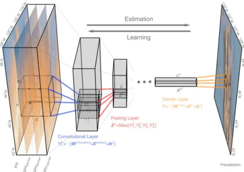
Figure 2.The convolutional neural network architecture for estimating precipitation using the numerical model resolved geopotential height and moisture field. The data are obtained from North American Regional Reanalysis Project data set. The stacked frames on the left side show the precipitable water (PW) and geopotential height (GPH) at 500, 850, and 1,000 hPa for the delineated 800 km×800 km region in Figure 1. The blue lines indicate a convolution operation applied on the circulation field. The red lines indicate the pooling operation that down-samples the local features. Several stages of convolution and pooling layers are stacked, followed by the fully connected dense layers (orange lines). The dense layer applies all the extracted features to estimate precipitation for the target geogrid, which is labeled on the precipitation map on the right part. The convolution and dense layers are optionally followed by a nonlinear transformationf, which are represented with semitranslucent fonts.
precipitation distribution are not well disintegrated and represented. While SD models are preferred to rec-ognize key circulation features of different appearances and locations, most existing statistical models make no explicit consideration of the cyclone depression intensity, coverage, and its distance to the target geogrid. To tackle these problems, we abide the “end-to-end” principle for extracting dynamical features and esti-mating precipitation. Specifically, the fine-scale circulation field resolved by numerical models is directly processed by the DNN to learn the representative features for precipitation estimation. Also, to disintegrate the impact of the cyclone geometric shape and position, we adopt the convolution mechanism in the network modeling. The method is explained in the following section.
4. Methodology
4.1. Convolutional Neural Network
CNNs share many similarities with regular neural networks. For a regular neural network, a statistical con-nection between the inputs and the outputs is constructed through hierarchical connected layers of neurons. Each neuron is a computing unit that receives some inputs, performs a dot product, and optionally fol-lows a nonlinear transformation. For supervised learning problems (i.e., classification and regression), a loss function is defined by comparing the network's output estimations with observations. The network param-eters are typically trained through minimizing the loss function using gradient descent, which is known as backpropagation training.
CNNs differ from regular neural networks in their connection manner for neurons within and between layers. In regular neural networks, each neuron is fully connected to all neurons in the previous layer, while neurons within a single layer do not share connections. For data that come in the form of multiple arrays, such as images and videos, there is strong correlation within neighboring patches and less considerable correlation between remote components. The local patterns contribute to large-scale patterns when they are inspected from a broader point of view. To extract and utilize the local features in neural network modeling, the full connection of neurons between successive layers becomes redundant, and local connection within
a single layer becomes imperative. To tackle this, the CNN explicitly encodes local connection and prohibits remote connection; also, the extracted local patterns are down-sampled to compose large-scale patterns. These operations are achieved using the convolution operator and pooling operator.
Below we use the precipitation estimation example to explain the idea of these operators. The storm event for the same geogrid in Figure 1 on 18:00 UTC, 7 November 2006 is used as illustration here. In Figure 2, the circulation and moisture field (left part) are fed into a CNN for extracting useful features and estimating the precipitation of the target geogrid (right part). The blue color indicates low values, and yellow indicates high values. A clear frontal system can be depicted as an occluded front forms around the mature low-pressure area. This is accompanied by copious precipitation falling along the warm conveyor belt, as shown in the precipitation map. These characteristic circulation patterns could appear in different geometrical shapes and at different locations. We expect that an explicit encoding of the local connectivity could enhance the extraction of the circulation geometries for precipitation estimation.
To extract the spatial salient features, the convolutional layer applies ac′ ×c×m×ntensor to go through the input with a predefined stride. Each convolution operation is performed by computing the element-wise dot product between the tensor and different patches of the input, which is represented as ac×x×yarray. Herecis the category of the predictors. Following previous works (Wilby & Wigley, 2000), the predictors consist of the circulation constraint and moisture constraint. The circulation constraint is represented by geopotential height (GPH) at different pressure levels. The moisture constraint is represented by the total column precipitable water (PW). The spatial coverage of the dynamical field is defined byxandy. The
c′×c×m×ntensor is named as kernel of the convolution layer, wherec′is the output channel number and
m×nrepresent thereceptive fieldof kernel. Each multiplication result is optionally followed by a nonlinear transformationf, such as the ReLU function:f(x) = max(0,x). The convolution operation can be interpreted as usingc′
filters to transform the input into a more representative form for the learning objective. Preferably, the network will learn filters that activate when they see critical local dynamical patterns on the first layer. Fostered by spatial down-sampling, which is achieved by the pooling operation, the network may eventually learn a synoptic atmospheric pattern that promotes precipitation on higher layers of the network.
The pooling layers act to coarsely grain local semantically similar features into one (LeCun et al., 1998). Through down-sampling, the higher layer convolutions work on extracted local features, which enables learning higher-level abstractions on the expanded receptive field (LeCun et al., 2015). A typical pooling unit computes the maximum of a local patch of units in one feature map. In Figure 1, we apply a 2 ×2 maximum pooling. For a typical CNN, several stages of convolution, nonlinearity, and pooling layers are stacked, followed by dense layers that apply all the extracted features for the learning target.
To estimate the total daily precipitation, we usually have several snapshots of its surrounding dynamical field at different hours through the day. Conventionally, these snapshots are averaged to reach a single picture of the general dynamical pattern for the daily precipitation estimation. Here, considering the fact that each circulation snapshot provides its information for a specific time of the day, we map the same CNN model on each of the dynamical field snapshot. Results from all the network computations are summed as the total daily precipitation estimation.
4.2. Regularization, Loss Function, and Training 4.2.1. Regularization
DNNs usually have much more complicated structures and more parameters than conventional ML algo-rithms, which make it possible for models to perform exceptionally well on the training data but predict the test data poorly. This phenomenon is called overfitting. Regularization refers to the strategies to avoid over-fitting and make the model generalize better to unseen data. We include the dropout (Srivastava et al., 2014) and batchnormalization (Ioffe & Szegedy, 2015) modules to enhance the model's performance.
The idea of dropout is to assign aprobability of existenceto the neurons and their associated connections. Thus, to train a DNN withnneurons is equivalent to train an ensemble of 2n“thinned” networks.
Dur-ing testDur-ing and applications, the weights are multiplied by the same probability of existence to offset the dropout effect. This prevents neurons from coadapting and has shown significant improvements in reducing overfitting (Srivastava et al., 2014).
Batchnormalization addresses the problem ofinternal covariate shiftin training DNNs. Specifically, the dis-tribution of each layer's inputs changes during the training process, which requires continuously adaption
and hinders the training process. Batchnormalization performs normalization of the output in the hidden layers (Ioffe & Szegedy, 2015). It has shown good performance in accelerating the training and regularizing the model in various DNN applications.
4.2.2. Loss Function and Skill Metrics
The root mean square error (RMSE) between the precipitation simulations and observations is used as loss function here: RMSE= √ 1 n ∑ (Pobser−Psimu)2. (2)
HerePobserdenotes the observed daily precipitation records, andPsimudenotes the simulated daily precipi-tation records.
The Pearson correlation coefficient (r) between simulated and observed daily precipitation is also used as supplementary skill metric for measuring model performance:
r= cov(Pobser,Psimu) 𝜎Pobser𝜎Psimu
. (3)
Herecovdenotes covariance, and𝜎denotes standard deviation. 4.2.3. Training
We apply backpropagation to train the network model here. The method requires estimating the partial derivative of the loss function with respect to each parameter in the network, including those from both the convolutional and dense layers. The parameters are then adjusted along the gradient descent direction by a predefined stride, which is named “learning rate.” A detailed derivation for backpropagation in CNN can be found in Bouvrie (2006).
Considering the fact that a same CNN is mapped to several snapshots of the dynamical field in a single day time, and their outputs are summed up as the final estimate of the daily precipitation, the gradient of the loss function is equally attributed to each snapshot before applying the backpropagation training.
4.3. Model Implementation
We implement the network using the Wolfram Mathematica V11.3 Deep Learning Platform (Wolfram, 2018). We use the Nvidia Quadro P5000 GPU (Graphics Processing Unit) to accelerate model training.
5. Experiments
5.1. Data
The predictors used for building the network models are the GPH and PW field data from the National Cen-ters for Environmental Prediction (NCEP) North American Regional Reanalysis (NARR) data set (Mesinger et al., 2006). The data set is generated by regional downscaling of the NCEP Global Reanalysis for the North America region, using the NCEP Eta Model and the 3-D Variational Data Assimilation System. Also, the updated Noah Land-surface model and numerous data sets additional to the global reanalysis were applied to improve the data quality. The data set covers 1979 to near present and is provided every 3 hr, with spatial resolution of 32 km/45 vertical layers. The 3-hr total column PW and GPH at 500, 850, and 1,000 hPa from 1979 to 2017 were downloaded for use.
Besides the pressure and moisture data, the precipitation product from the NARR is used as baseline here. It should be noted that the NARR precipitation product is not raw output from the numerical models but is achieved by assimilating precipitation observations as latent heating profiles (Lin et al., 1999). Thus, the data quality is superior to the raw numerical precipitation estimates or conventional reanalysis precipitation products that do not assimilate precipitation (Becker et al., 2009; Bukovsky & Karoly, 2007). It poses a high challenge for the DNN model to provide comparable precipitation estimates.
We use the gage-based daily precipitation data set from the National Oceanic and Atmospheric Adminis-tration (NOAA) Climate Prediction Center (CPC; Xie et al., 2010) as the “realistic” precipitation records for training and test the CNN. The data set provides high-quality unified precipitation records by combining dif-ferent information sources. It covers 1948 to 2017 with resolution of 0.25◦ ×0.25◦. The data are resampled to 32 km using nearest neighbor method to match the resolution of NARR.
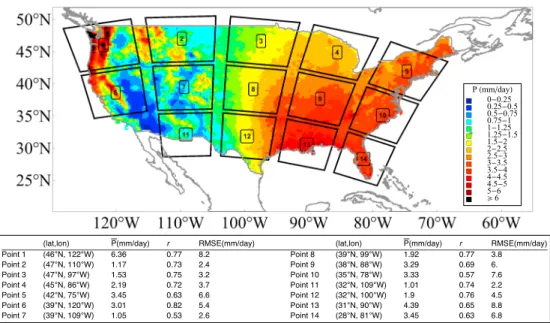
Figure 3.The sample grids used in the experiment. For each grid, the surrounding800km×800km dynamical field is delineated. The color indicates the mean daily precipitation rate, which is calculated by averaging the CPC daily precipitation records from 1979 to 2017. The table shows the samples' coordinates, mean precipitation rate, ther, and root mean square error (RMSE) between North American Regional Reanalysis Project and Climate Prediction Center precipitation for the grids.
5.2. Experiments Design
To test the applicability of the model for different climate conditions, we selected 14 sample grids that roughly cover the characteristic climate divisions of the contiguous United States. The samples together with their associated circulation field domains are shown in Figure 3. The circulation field for each gird is composed of a 8×4×25×25tensor. Eight indicates that there are eight 3-hr circulation snapshots per day; 4 indicates the feature numbers, which includes the PW,GPH1000hPa,GPH850hPa, and GPH500hPa; 25 × 25 represents that there are 25×2532-km grids within the considered dynamical field coverage.
For each sample grid, we carry out the following steps to build the model:
1. Data normalization. Each feature field is normalized by subtracting the mean (𝜇) and dividing by the standard deviation (𝜎). Here𝜇and𝜎are scalar values that are calculated based on the flattened circulation field for the entire data set. The grids are not normalized individually in order to maintain the circulation structure.
2. Divide the data into training, validation, and test sets. To guarantee each set covers different climate con-ditions, for each of the 12 months, we randomly select 23 years of that particular months data into the training set, 6 years into validation set, and 10 years into test set. Thus, we have 23/6/10 years' recomposed data in the training/validation/test set. The training and validation sets are used to calibrate the model parameters and prevent overfitting. The test set is kept unseen through the training process. It is used to provide an unbiased evaluation of the constructed model.
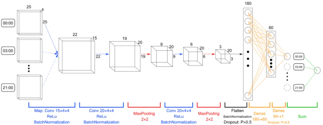
3. Determine the network hyperparameters. Hyperparameters are the variables that determine the network structure (i.e., layer type and neuron size) and the variables that determine how the network is trained (i.e., the learning rate; Goodfellow et al., 2016). We adapt the architecture of a classical CNN implementation named LeNet (LeCun et al., 1998) in determining the hyperparameters. The specific network structure is shown in Figure 4. Based on this basic model architecture, we focus on one sample grid and implement a series of architecture variations to figure out the best network structure configuration and attribute the contribution to the adjusted modules.
4. Train the network. The parameters in the network are first initialized based on standard normal distri-bution. To guarantee model's robustness with respect to parameter initialization, we carry out several implementations with different parameter initializations. After initialization, the parameters are further trained using stochastic gradient descent (Bottou, 2010) to minimize the MSE for precipitation estimate. The stochastic gradient descent method applies a stochastic approximation of gradient descent approach
Figure 4.The network structure for precipitation estimation. Each 3-hr snapshot of the dynamical field, which is represented by a 4×25×25 tensor, is sequentially processes through the convolutional and pooling layers. The extracted features are flattened and processes by two consecutive dense layers. The dimension of each layer's output is labeled out. Different layers/operators are denoted with corresponding colors. Results for eight 3-hr snapshots are summed as the total daily precipitation estimate. In total, this network consists of 24,076 parameters to be trained.
to alleviate the high computing cost in evaluating the derivatives for the global loss function. The consid-ered learning rate are 10−2,10−4, and 10−6. We adopt the early stopping strategy to regularize the model: The training process is terminated when further training improves performance only for the training set but not for the validation set.
5. Model evaluation. The network simulation results are evaluated against the CPC precipitation records, using skill metrics of RMSE andr. The performance are compared against the original NARR precipitation products.
6. Results
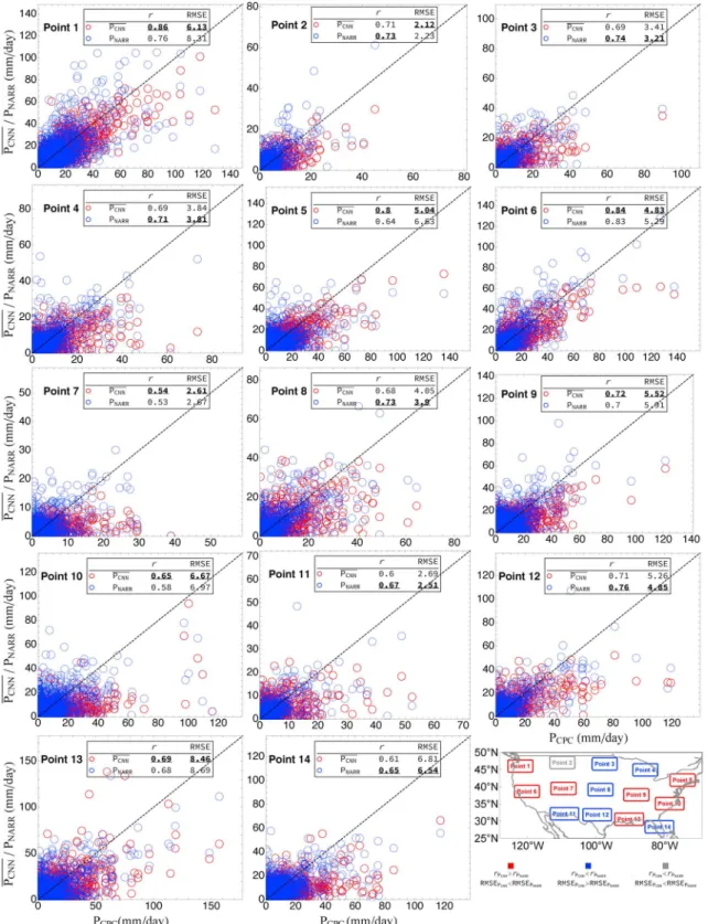
The CNN estimated precipitation (PCNN) and the NARR estimated precipitation (PNARR) are compared against the CPC precipitation records. Figure 5 shows the comparison results for the test set. Here PCNNis the mean estimation from three CNN implementations with different parameter initializations.
Without a careful tuning of hyperparameters, the CNN models perform relatively well compared to the NARR precipitation product. Considering the fact that the NARR precipitation product has already assimilated observations, the results are quite satisfactory.
As indicated by the two skill scores, PCNNoutperforms PNARRfor most sample points from the west and east coast, where precipitation is more copious than the other areas. The skill improvement is impressive for some of the sample points. For instance, for point 5,r/RMSE improves from 0.64/6.63 to 0.80/5.04 comparing PCNNwith PNARR. For the rest sample points from the middle part of the continent, PCNNperforms slightly worse compared to PNARR. Particularly, the CNN models show systematic underestimation for the large precipitation events.
Table 1 shows the skill scores ofrand RMSE for the training, validation, and test set for each of the three CNN implementations carried out here. The skill scores of CNN ensemble prediction and NARR precipitation product are also included for comparison purpose.
Compared to individual implementations of CNN, the ensemble estimation of CNN (CNNR) improves the skill scores in most cases . However, the improvement is generally not significant. Different implementations of CNN show similar skills. This indicates that the parameter initialization carried out here does not signif-icantly influence the modeling performance; in other words, the model is robust with respect to different parameter initializations.
Considering the performance difference for the training, validation, and test sets, as can be expected, all points show better performance of CNN models for the training set compared to the validation and test sets. The overfitting phenomena are assumed to be responsible for the relatively poorer performance for the CNN models in the middle part of the continent. For instance, for point 3,rP
CNN is 0.80/0.69/0.69 for the training/validation/test set, whilerPNRAA is 0.76/0.71/0.74. The overfitting may due to the fact that for
Figure 5.The scatter plots compare thePCNN(red circles) /PNARR(blue circles) against the Climate Prediction Center precipitation records (Pobser) for the 14 sample points. Results are for the test set only. The skill scores ofrand root mean square error (RMSE) for each point are given in corresponding subfigures. The bold and underlined value indicates the better statistics of the two estimates. The bottom right geographic map shows the geoposition of the 14 points. The point is labeled red/blue if both skill scores indicate thatPCNN/ PNARRperforms better. It is labeled gray if the two skill scores show disagreement.
Ta b le 1 Pr ecipitation E stimation S kills of CNN a nd N A RR for the T raining/V alidation/T est Set T raining V a lidation T est CNN R1 CNN R2 CNN R3 CNN R N A RR CNN R1 CNN R2 CNN R3 CNN R N A RR CNN R1 CNN R2 CNN R3 CNN R NA R R Po in t 1 r 0 .90 .9 10 .9 0 . 91 0.78 0.85 0.85 0.85 0 . 86 0.74 0.85 0.85 0.85 0 . 86 0.76 RMSE 5.39 5.1 5 .47 5 . 15 8.17 5.97 6. 5.99 5 . 81 8.18 6.23 6.35 6.3 6 . 13 8.31 Po in t 2 r 0.79 0.82 0.79 0 . 82 0.74 0.63 0.64 0.65 0.66 0 . 71 0.67 0.7 0 .68 0 .71 0 . 73 RMSE 2.14 2 . 04 2.13 2.05 2.38 2.52 2.49 2.48 2.44 2 . 43 2.21 2.15 2.2 2 . 12 2.23 Po in t 3 r 0.78 0.78 0.8 0 . 8 0.76 0.68 0.66 0.68 0.69 0 . 71 0.67 0.68 0.67 0.69 0 . 74 RMSE 3.03 3.1 2 .94 2 . 94 3.26 3.29 3.35 3.29 3 . 23 3.26 3.48 3.48 3.53 3.41 3 . 21 Po in t 4 r 0.78 0.77 0.78 0 . 79 0.72 0.73 0.71 0.68 0.72 0 . 76 0.68 0.66 0.66 0.69 0 . 71 RMSE 3.23 3.25 3.26 3 . 14 3.61 3.72 3.81 3.97 3.73 3 . 55 3.89 3.98 3.96 3.84 3 . 81 Po in t 5 r 0.82 0.8 0 .8 0 . 82 0.63 0.76 0.75 0.74 0 . 76 0.62 0.78 0.79 0.79 0 . 8 0.64 RMSE 4.74 4.92 5. 4 . 74 6.58 5.36 5.43 5.56 5 . 3 6.56 5.24 5.17 5.17 5 . 04 6.63 Po in t 6 r 0.91 0.92 0.93 0 . 93 0.82 0.82 0.82 0.83 0 . 83 0.82 0.84 0.84 0.82 0 . 84 0.83 RMSE 3.76 3.64 3 . 29 3.41 5.47 4.88 4.89 4.78 4 . 7 5.24 4.96 4.89 5.19 4 . 83 5.29 Po in t 7 r 0.59 0.58 0.59 0 . 61 0.53 0.53 0.54 0.52 0 . 55 0.52 0.53 0.51 0.51 0 . 54 0.53 RMSE 2.32 2.36 2.37 2 . 31 2.54 2.8 2 .79 2 .86 2 . 78 2.98 2 . 6 2.64 2.68 2.61 2.67 Po in t 8 r 0 . 79 0.75 0.75 0.78 0.77 0.71 0.71 0.71 0.73 0 . 86 0.67 0.66 0.66 0.68 0 . 73 RMSE 3 . 77 3.99 4.01 3.82 3.89 4.66 4.56 4.57 4.51 3 . 31 4.12 4.18 4.16 4.05 3 . 9 Po in t 9 r 0.74 0 . 79 0.76 0.78 0.7 0 .72 0 .72 0 .7 0 . 73 0.65 0.7 0 .71 0 .71 0 . 72 RMSE 5.6 5 . 23 5.44 5.31 6.11 5.27 5.29 5.41 5 . 19 6. 5.65 5.64 5.61 5 . 52 5.91 Po in t 1 0 r 0 . 75 0.65 0.66 0.71 0.6 0 .54 0 .54 0 .54 0 . 57 0.47 0.57 0.63 0.62 0 . 65 0.58 RMSE 7.79 7 . 11 7.23 7.12 7.56 8.95 8 . 13 8.24 8.27 8.76 7.52 6 . 47 6.67 6.67 6.97 Po in t 1 1 r 0.72 0.71 0.71 0.73 0 . 77 0.66 0.62 0.61 0.65 0 . 75 0.6 0 .58 0 .59 0 .6 0 . 67 RMSE 2.2 2 .25 2 .25 2 .18 2 . 04 2.74 2.86 2.88 2.77 2 . 4 2.7 2 .79 2 .74 2 .69 2 . 51 Po in t 1 2 r 0.8 0 .75 0 .79 0 . 8 0.74 0.74 0.71 0.7 0 .74 0 . 8 0.7 0 .67 0 .69 0 .71 0 . 76 RMSE 3 . 76 4.2 3 .9 3.8 4 .36 5 .07 5 .29 5 .32 5 .07 4 . 49 5.37 5.58 5.45 5.26 4 . 85 Po in t 1 3 r 0.82 0.82 0.77 0 . 82 0.65 0.69 0.72 0.7 0 . 72 0.59 0.67 0.66 0.68 0 . 69 0.68 RMSE 6.52 6.5 7 .17 6 . 44 8.77 8.15 7.8 7 .98 7 . 76 9.39 8.68 8.86 8.69 8 . 46 8.69 Po in t 1 4 r 0 . 69 0.64 0.67 0.68 0.64 0.62 0.62 0.62 0 . 63 0.59 0.61 0.59 0.58 0.61 0 . 65 RMSE 6 . 08 6.48 6.29 6.15 6.68 6.97 7. 7.03 6 . 87 7.36 6.79 6.96 7.02 6.81 6 . 54 No te . CNN = con volutional neur al network; N A RR = N orth American R egional R eanalysis Pr oject; R MSE = root mean squar e err or . R 1, R2, a nd R3 indicate 3 implem entations o f CNN with differ ent par a meterization initializations. R re pr esents the m ean estimation. The b old a nd underlined va lues indicate the b est statistics for corr esponding d ata set.
Table 2
Model Performances for Different Receptive Fields and Convolution Depth
Receptive field Convolution depth
1×1 3×3 4×4a 5×5 6×6 Full 1 3a 5 7 Training 0.869 0.885 0.902 0.922 0.939 0.864 0.837 0.902 0.921 0.887 r Validation 0.836 0.848 0.851 0.853 0.836 0.824 0.811 0.851 0.850 0.837 Test 0.832 0.847 0.851 0.854 0.847 0.822 0.808 0.851 0.853 0.838 Training 6.11 5.78 5.32 4.79 4.59 6.29 7.01 5.32 4.82 5.73 RMSE Validation 6.25 6.05 5.99 5.95 6.36 6.55 6.94 5.99 6.02 6.27 Test 6.6 6.37 6.29 6.25 6.49 6.85 7.32 6.29 6.27 6.58
Note. RMSE = root mean square error. The bold and underlined values indicate the best statistics for corresponding experiments.
aThe skill scores for the default settings (receptive field:4×4; convolution depth: 3) are the averaged scores for the three implementations in the previous section.
this subarid region, there are much less samples of precipitation events compared to the rest areas. The limited informative data cannot effectively support the construction of a complicated DNN model. Despite the overfitting, the CNN models have relatively similar performance for the validation and test set, which guarantees the trained model can generalize well to the unseen data.
Another important aspect we noticed is that the CNN models frequently underestimate large precipitation values. We believe the underestimation might be caused by the following reasons: First, we do not have enough large precipitation samples due to the uneven distribution of daily precipitation; second, the convec-tive storms, which are common for the east and southeast of the continent, might require finer dynamical field for accurate estimation.
7. Discussion
7.1. Network Architecture
The results above are achieved using a same default network architecture as presented in Figure 4. To (1) attribute the credits to the introduced modules, (2) figure out their optimal configurations, and (3) relate our models to the classical ANN SD approaches, we implement a series of network architecture variations based on the default network structure.
Given the complexity of DNN structures and huge computing cost for model training, it is impractical to enumerate all the possible network architecture compositions. Here we focus on two dominant configura-tions in CNN design, namely, thereceptive fieldand thenetwork depth. For processing convenience, we use a single geogrid to carry out the experiments. The geogrid of point 1 is selected since we have made detailed descriptions for it.
7.1.1. Receptive Field: Extensive Or Exclusive?
The receptive field for a convolutional layer refers to the patch size on which the kernel convolve with. In Figure 2, it is denoted asm ×n. It constrains the spatial scale of the features that we expect to extract through convolution. Large-scale spatial features can be achieved either by adopting a big receptive field on the initial layers or assembling local features in deeper layers.
Consider the extreme condition of applying the most extensive receptive field, that is,m = xandn = y
for the case in Figure 2, all the pixels in the input layer are thus fully connected. The CNN degenerates to a regular fully connected neural network, which has been extensively applied in ANN SD. Considering another extreme condition of applying the most exclusive receptive field, that is,m = 1andn = 1, the one-by-one convolution performs a coordinate-dependent transformation in the filter space, which has been used to modify the dimensionality in the channel dimension (Lin et al., 2013; Szegedy et al., 2015). We carry out the experiments by modifying the receptive field for all the convolutional layers. We maintain the two other network configurations the same as the default setting. As is shown in Figure 4, originally, a 4×4receptive field is adopted for all of the three convolutional layers. Here we consider the receptive field of 1×1,3×3,5×5,6×6, and full input size (25×25for the first convolutional layer and 1×1for the rest). The results are shown in Table 2.
For point 1, the best training set performance is achieved when using a receptive field of 6 × 6, while the best validation/test set performance is achieved when using a receptive field of 5 × 5. The two extreme condition experiments achieve poorer performance than the others. The one-by-one convolution network works better than the full receptive field network or, in other words, the fully connected neural network. It should be noted that the optimal receptive field size might be different for areas with different precipitation mechanisms.
Physically, precipitation is highly variant in space. Its occurrence and intensity are closely related to local circulation patterns. The above experiments verified that an explicit encoding of local spatial circulation structures enhances the estimation of precipitation.
7.1.2. Network Depth: Shallow Or Deep?
The network depth can be roughly represented as how many layers there are in the neuron network. These layers learn representations of the data with multiple levels of abstraction (LeCun et al., 2015). Despite the simplicity of the transformation in each layer, the stacking of many layers allows learning intricate structures for complicated applications.
Here we apply a relatively shallower CNN model and two deeper CNNs to examine the impact of network depth. The shallower CNN model is constructed by removing the latter two convolutional layers and the last pooling layer from the default network in Figure 4. Thus, its convolution depth is 1. The deeper CNN models are constructed by adding two/four extra convolutional layers before the first pooling layer for the default network architecture in Figure 4. The kernel size of the included convolutional layers is set to 20×c×4×4, wherecis the channel number of the previous layer. The deeper networks are thus of convolution depth of 5/7. The performance of the models are also presented in Table 2.
Compared to the deeper network models, the model with single convolutional layer achieves significant lower skill scores in estimating precipitation. The default network with three convolutional layers achieves optimal performance for the validation set. The model with 5 convolutional layers achieves optimal perfor-mance for the training and test set. Overall, results indicate that the shallow network is not as effective as the deeper networks in extracting useful dynamical features for precipitation estimation. Ideally, the deeper networks hold more potential in estimating the intricate features. However, results here show that the net-work with seven convolutional layers achieve lower skill score than the netnet-works with 3/5 convolutional layers. This might due to inefficient backpropagation training for such a deep network model.
7.2. Model Interpretations
The network models applied here involve much more complicated structures and more parameters com-pared to the existing SD approaches. It is imperative to explain what is learned through adopting these network components, and how the network can learn better. In response to this requirement, many approaches for understanding CNNs have been developed in recent years (Erhan et al., 2009; Simonyan et al., 2013; Zeiler & Fergus, 2014). Here we apply two commonly used visualization and analysis methods to interpret the models and their results.
7.2.1. Layer Activation
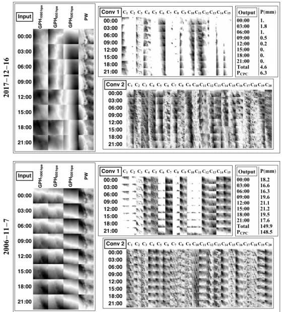
Layer Activation refers to setting break points in the middle layers of the network and visualize the activated outputs at these break points. Zeiler and Fergus (2014) offered an excellent example in illustrating how layer activation can be used for interpreting and diagnosing CNNs. We visualize the layer activations of the storm event in Figure 1 as well as a light rain event on 16 December 2017. Results are shown in Figure 6. The input fields for the two events in Figure 6 show different spatial structures. However, it is difficult to tell how these patterns are related to precipitation. The outputs from the first convolutional layer (Conv 1) provide a sharper distinction for the heavy/light precipitation events: For certain channels, the outputs for one event are activated while the outputs for the other event are not. For instance, the light precipitation event shows high spatial variance in the channels ofC3,C6,C10, andC11; for the storm event, there are little spatial variance in these channels; on the other hand, the light precipitation event shows little spatial variance in the channels ofC5,C7,C9,C13,C14, andC15; for the storm event, there are high spatial variance in these channels. The results in Conv 1 are further processed through deeper layers. Similar distinctions within same channel for two events can be depicted in Conv 2. Overall, the results here provide supportive evidences that the CNN models enhance the extraction of characteristic features by filtering the data with the learned kernels.
Figure 6.Layer activations for the 16 December 2017 light precipitation event (top) and 7 November 2006 storm event (bottom). The dark color represents low values, and bright color represents high values. The left part shows the eight 3-hr snapshots of the dynamical field (GPH1,000 hPa,GPH850 hPa,GPH500 hPa, and PW) through the day. Conv 1/2 shows the activated output for the first/second convolutional layer. The Conv 1 result is composed of8×15subfigures. Eight indicates that there are eight 3-hr dynamical field snapshots; 15 indicates that the output is of 15 channels, which are labeled as fromC1toC15. Similar denotations for Conv 2. The Output panel shows the results by mapping the convolutional neural network to each 3-hr snap shot of the dynamical field. The sum of them consists the total daily precipitation estimate, which is compared against CPC records. PW = precipitable water; GPH = geopotential height.
7.2.2. Perturbation Sensitivity
For image classification problems, the occlusion sensitivity analysis tells the impact of different portions of the image on the classification result. It is performed by systematically occluding different portions of the input image with a gray square and monitoring the output of the classifier (Zeiler & Fergus, 2014). The results of occlusion sensitivity analysis illustrate if the model is effectively localizing the target object in the image, or just using the surrounding context.
For the problem here, we apply a similar method to quantify the precipitation-related impact of different portions of the circulation field. Rather than applying a gray square to occlude the input, we systematically perturb the input field with a rescaling matrix. The dimension of the rescaling matrix is set to be the same as the receptive field for the first convolutional layer. All of its elements are set to 1+𝜖, where𝜖is the perturba-tion magnitude. The rescaling matrix is multiplied to different porperturba-tions of the input. For each perturbaperturba-tion,
Figure 7.Perturbation sensitivity analysis for the 16 December 2017 light precipitation event (top) and 7 November 2006 storm event (bottom). For each case, we visualize the model output changes by systematically perturbing different portions of the scene with a rescaling matrix that is of same dimension as the first convolutional layer receptive field. The perturbation magnitude is set to 5%. The results are denoted as𝜕 𝜕P
Dynamics. We provide clear 2-D projections of these
figures in the supporting information. GPH = geopotential height; CNN = convolutional neural network.
we monitor the model output change. Mathematically, this operation is roughly equivalent to estimating the partial derivatives of the precipitation estimate with respect to different portions of the dynamical field. The relation between perturbation location and model output change is visualized in Figure 7.
In Figure 7, as we slide the scaling matrix over different geolocations in different species of the dynamical fields, the model estimated precipitation amount changes correspondingly. For instance, for the 2007-11-7 storm event, the CNN model will produce larger precipitation estimate if the 1,000-hPa GPH for the central region is lower and the 1,000-hPa GPH for the surrounding area is higher. This is in accordance with our prior knowledge that heavy precipitations are related to intensive surface depressions. It is interesting to
Table 3
Precipitation Estimation Performance for the Test Set Using (1) Linear Regression, (2) Nearest Neighbor, and (3) Random Forest Model
Input Skill score Linear regression Nearest neighbor Random forest
2 PCs r 0.74 0.80 0.80 (4×2) RMSE 8.01 7.35 7.23 8 PCs r 0.79 0.81 0.81 (4×8) RMSE 7.33 7.34 7.05 16 PCs r 0.81 0.81 0.81 (4×16) RMSE 6.98 7.50 7.09 64 PCs r 0.81 0.58 0.80 (4×64) RMSE 7.03 11.2 7.19 256 PCs r 0.76 0.67 0.80 (4×256) RMSE 8.86 12.47 7.19 Raw Input r 0.52 0.79 0.81 (4×25×25) RMSE 10.35 7.41 7.04
Note. RMSE = root mean square error. For each model, we carry out simulations using input composed of the leading 2, 8, 16, 64, and 256 principal components (PCs) of the circulation field data, as well as simulations using the raw circulation field data. The dimension for the input variable is labeled; for instance,4×2indicates that the leading 2 PCs for the GPH1,000 hPa,GPH850 hPa,GPH500 hPa, and PW field are used as input. Therand RMSE score are used to measure model performance.
note that the perturbation sensitivity map occasionally presents the characteristic appearances of cyclones. Overall, the precipitation estimations are highly sensitive to the dynamics from the central region of the field. This is the area where the target geogrid point lies. The surrounding dynamics also provide important context for inferring precipitation.
7.3. Comparison Experiments
Previous sections have compared the CNN precipitation estimates with (1) NARR precipitation product and (2) precipitation estimates using fully connected DNN. Results show that the convolution module enhances DNNs for precipitation estimate, achieving advanced performance compared to observation-adjusted numerical precipitation product.
In section 3, we made a critical review on existing SD approaches, which motivates us to turn to CNN for explicit encoding of precipitation-related circulation geometric patterns. To justify the critics and the moti-vation, it is imperative to compare the CNN performance with classical SD approaches. Here we carry out a series of comparison experiments using some of the widely adopted SD methods.
We select the following SD models as baselines : (1) linear regression, (2) nearest neighbor, and (3) ran-dom forest, all of which have been extensively applied and verified for SD tasks (Gangopadhyay et al., 2005; Hutengs & Vohland, 2016; Li & Smith, 2009). For each of the model, we adopt same input variables as for CNN, with optional feature extractions before feeding the input to the model. The data normalization, par-tition of training/validation/test set, is the same as in the CNN experiment. The optional feature extraction is done using principal component analysis. We carry out simulations using input composed of the leading 2, 8, 16, 64, and 256 PCs of the circulation field data, as well as simulations using the raw circulation field data. Details of the models and feature extraction are given in the supporting information (Breiman, 2001; Louppe, 2014; Wolfram, 2018; Pearson, 1901; Shlens, 2014). The precipitation estimation results for the test set are shown in Table 3.
The best performance in the comparison experiments is achieved by the linear regression model using input of the leading 16 PCs of the circulation field (r = 0.81,RMSE = 6.98). The nonlinear models outperform linear model when the input dimension is relatively low. As we include more PCs as input, the skills for the models decrease (linear regression and nearest neighbor) or saturate (random forest).
The performance of the models here are comparable or slightly better than the NARR precipitation estimates (r = 0.76,RMSE = 8.31). DNN with fully connected computation graph achieves better performance (r = 0.82,RMSE = 6.85). The skill can be further improved if we apply the convolution and pooling
modules to explicitly extract the spatial information from the high-dimensional dynamical field (r = 0.86,RMSE = 6.13). To sum up, the comparison experiments empirically suggest that CNN is competitive in making precipitation estimations based on the resolved surrounding atmospheric dynamics.
8. Conclusion
Precipitation estimation provides fundamental information to better understand the land-atmosphere water budget, improve water resources management, and aid in preparation for increasingly extreme hydrome-teorological events. However, the precipitation process is generally considered to be poorly represented in current numerical weather/climate models.
SD approaches often provide more accurate precipitation estimates compared to the raw precipitation products in numerical models. However, we point out two common deficiencies in adopting the exist-ing precipitation SD approaches for daily precipitation estimation: First, most existexist-ing SD approaches rely on human-engineered features to extract information from the raw form high-dimensional predictors, such as the PCs; however, the engineered features are often designed based on the characteristics of the predictors rather than the connections between the predictors and the precipitation process; second, the cir-culation geometries and positions that dominant precipitation distribution are not well disintegrated and represented.
We introduce the CNN model to overcome these two deficiencies in improving precipitation estimation. The CNN model stacks several convolution and pooling operators to extract the intricate but important circula-tion features for precipitacircula-tion estimacircula-tion. Instead of applying pre-engineered feature extractors, the model applies “end-to-end” learning. Specifically, the kernels that are used to extract the salient features from the resolved dynamical field are optimized by backpropagating the precipitation estimation error through the convolutional layers. Thus, the learned features are determined based on the relation between the predic-tors and the predictand for the exact learning target. Also, through hierarchical convolution, we can well disintegrate dominant circulation features of different geometric properties and from different locations. The model is tested for 14 geogrid points that roughly cover different characteristic climate divisions of the contiguous United States. We use the every 3-hr GPH and PW field from the NARR data set to provide realistic and fine-scale dynamical forcing. The CNN models are implemented by connecting the dynamical forcings with the CPC gage-based daily precipitation records. Considering the fact that each 3-hr snapshot of the dynamical field provides specific information for the particular time of a day, we map the CNN network to each 3-hr snapshot and sum up the results as the daily precipitation estimate. The parameters of the network are trained by minimizing the estimation error using backpropagation.
Results show that the CNN model outperform original NARR precipitation estimates for the west and east coast, where precipitation is more copious compared to the other areas. For the middle part of the continent, the CNN model shows slightly worse performance, which can be attributed to model overfitting when there are limited precipitation samples for training the model.
We focus on a single geogrid point to examine the influence of the network architecture on model perfor-mance. Specifically, we focus on the receptive field and network depth. By varying the receptive field of the convolutional layers, we verify that the CNN model outperforms conventional fully connected ANN SD in estimating precipitation through explicit encoding of local spatial circulation structures. By varying the net-work depth, we found that deep netnet-works generally have better performance compared to shallow netnet-works. However, we also noticed the difficulty for training very deep networks.
To interpret the model, we visualize the activation of the middle layers of the network using a storm event and a light precipitation event. Results show that different channels are activated for the two cases of differ-ent dynamical condition and precipitation amount. We also implemdiffer-ent the perturbation sensitivity analysis to quantify the precipitation-related impact of different portions of the dynamical field.
We compare the model performance with some of the widely adopted SD methods, including linear regres-sion, nearest neighbor, and random forest. Results show that the CNN model outperforms the baseline SD approaches for accurate precipitation estimates.