Using molecular QTLs to identify cell types and causal variants for complex traits

(1)

Using molecular QTLs to identify cell types

and causal variants for complex traits

Jeremy Schwartzentruber

Wellcome Trust Sanger Institute

Clare College

University of Cambridge

This dissertation is submitted for the degree of Doctor of Philosophy

October 2017

(2)

(3)

Declaration of Originality

This dissertation is the result of my own work and includes nothing which is the outcome of work done in collaboration except as declared in the beginning of each chapter. It is not substantially the same as any that I have submitted, or, is being concurrently submitted for a degree or diploma or other qualification at the University of Cambridge or any other

University or similar institution. I further state that no substantial part of my dissertation has already been submitted, or, is being concurrently submitted for any such degree, diploma or other qualification at the University of Cambridge or any other University of similar institution. This dissertation does not exceed the word limit set by the Degree Committee for the Faculty of Biology.

Signature:

Date:

Jeremy Schwartzentruber October 2017

(4)

(5)

Abstract

Genetic associations have been discovered for many human complex traits, and yet for most associated loci the causal variants and molecular mechanisms remain unknown. Studies mapping quantitative trait loci (QTLs) for molecular phenotypes, such as gene expression, RNA splicing, and chromatin accessibility, provide rich data that can link variant effects in specific cell types with complex traits. These genetic effects can also now be modeled in

vitro by differentiating human induced pluripotent stem cells (iPSCs) into specific cell types,

including inaccessible cell types such as those of the brain. In this thesis, I explore a range of approaches for using QTLs to identify causal variants and to link these with molecular functions and complex traits.

In Chapter 2, I describe QTL mapping in 123 sensory neuronal cell lines differentiated from human iPSCs. I observed that gene expression was highly variable across iPSC-derived neuronal cultures in specific gene categories, and that a portion of this variability was explained by commonly used iPSC culture conditions, which influenced differentiation efficiency. A number of QTLs overlapped with common disease associations; however, using simulations I showed that identifying causal regulatory variants with a recall-by-genotype approach in iPSC-derived neurons is likely to require large sample sizes, even for variants with moderately large effect sizes.

In Chapter 3, I developed a computational model that uses publicly available gene expression QTL data, along with molecular annotations, to generate cell type-specific probability of regulatory function (PRF) scores for each variant. I found that predictive power was improved when the model was modified to use the quantitative value of annotations. PRF scores outperformed other genome-wide scores, including CADD and GWAVA, in identifying likely causal eQTL variants.

In Chapter 4, I used PRF scores to identify relevant cell types and to fine map potential causal variants using summary association statistics in six complex traits. By examining individual loci in detail, I showed how the enrichments contributing to a high PRF score are transparent, which can help to distinguish plausible causal variant predictions from model misspecification.

(6)

(7)

Acknowledgements

I have been fortunate to spend the past four years at the Wellcome Genome Campus, a place with many inspired scientists whose door is always open. Firstly, I would like to thank my supervisor Dan Gaffney, for allowing me to explore different project and ideas; for being involved every step of the way; for his commitment to think carefully about each claim we make; and for his focus on clearly explaining why. I am also grateful to members of our group - Kaur, Natsuhiko, Angela - who so readily shared their thoughts and expertise with me, as well as their code. I benefited greatly from the collaborative and supportive

environment at the Sanger Institute, including discussions with Jeff Barrett, Leo Parts, Carl Anderson, Annabel Smith, and Christina Hedberg-Delouka, as well as Chris Wallace in Cambridge. A big thank you Alex Gutteridge, for his cheerfulness, clear code and helpfulness in many analyses.

Thanks also to the other PhD students who always included me and played so well with Maia (junior PhD13 member who grew up from 0 to 4 years old on campus). I wish you all the best Katie, Nicola, Sumana, John, Masha, Li Meng, Veli, Liliana, Alice!

I am grateful to Dr. Jenny Clapham, who was one of the few doctors that seemed to take the chronic pain that I suddenly developed seriously. It was a dark ~1.5 years of my life, and a doctor who believes what you say and trusts you can make such a difference, even when there are no clear answers.

Finally, thank you to my two little girls for the many delightful moments. To Neeltje for supporting me and our girls through both delightful and difficult moments, and for

shouldering the lack of sleep! To Kees and Michalien for being so quick to help, so steadfast, and calm. And to my parents, for always listening to me and supporting me no matter what.

(8)

(9)

Abbreviations and key terms

ATAC Assay for transposase-accessible chromatin

AUC Area under the curve (used for ROC or other classifier metrics) BAM Binary sequence alignment file format

BF Bayes factor

CADD Method predicting deleteriousness of coding and non-coding variants CAGE Cap analysis of gene expression

caQTL Chromatin accessibility QTL

CD Crohn's disease

ChIP-seq Chromatin immunoprecipitation followed by sequencing

CNS Central nervous system

CQN Conditional quantile normalization for gene expression CV Coefficient of variation (standard deviation / mean) DNase I Enzyme that preferentially cuts DNA at open chromatin

DRG Dorsal root ganglion

E8 Essential 8 iPSC culture medium

eGene eQTL gene

eQTL Gene expression QTL

ESC Embryonic stem cell

FANTOM Dataset of TSS usage based on CAGE

FDR False discovery rate

fgwas A fine-mapping method incorporating functional genomic annotations FPKM Fragments per kilobase of exon per million mapped reads

GERP Genomic evolutionary rate profiling, a sequence conservation metric GTEx Genome-tissue expression project

GWAS Genome-wide association study

GWAVA Method predicting deleteriousness of non-coding variants HDL High density lipoprotein

HGMD Human gene mutation database

HIPSCI Human induced pluripotent stem cell initiative

IBD Inflammatory bowel disease

iPSC Induced pluripotent stem cell IPSDSN iPSC-derived sensory neuron LCL Lymphoblastoid cell line

LD Linkage disequilibrium

LDL Low density lipoprotein

LLK Log-likelihood (of a model, given certain parameters)

(10)

MEF (feeder) Mouse embryonic fibroblast "feeder" cell MPRA Massively parallel reporter assay

PPA Posterior probability of association PRF score Probability of regulatory function score

QC Quality control

QTL Quantitative trait locus

RA Rheumatoid arthritis

ROC Receiver operating characteristic evaluation metric for classifiers RPKM Reads per kilobase of exon per million mapped reads

SC3 Single cell consensus clustering method

SCZ Schizophrenia

SNP Single nucleotide polymorphism

sQTL Gene splicing QTL

TAD Topologically associating domains

TF Transcription factor

TFBS TF binding site

TPM Transcripts per million TSS Transcription start site

UC Ulcerative colitis

UTR Gene untranslated region

WGS Whole genome sequencing

(11)

1 Introduction

A decade ago, large-scale genome-wide association studies (GWAS) conducted as part of the Wellcome Trust Case Control Consortium led to the discovery of 24 genomic loci

associated with common human diseases (Wellcome Trust Case Control Consortium 2007). Prior to this, linkage mapping in human pedigrees had been successful in identifying genes and genetic variants leading to Mendelian diseases, but had largely failed for complex traits. Although the amount of phenotypic variation explained by these GWAS associations was small, they provided the first unbiased, genome-wide view of the genetic architecture of complex traits. Since then, GWAS have been done with increasing sample sizes for many human traits, leading to thousands of genomic loci associated with hundreds of traits. However, at the vast majority of these loci the causal variants and molecular mechanisms are uncertain. At present, most GWAS associations only represent leads into a wealth of underlying biology that will require new data and new methods to unravel. If we can do so, there is the promise that they will lead to a new understanding of complex traits, and new treatments for common diseases that together affect a large fraction of the population.

In this chapter, I outline the reasons that determining the causal variants and mechanisms behind GWAS associations is so challenging. I discuss how studies of molecular traits can provide insight into the functionality of different genomic regions, and introduce the reference datasets that many of my analyses are based on. Some human cell types are difficult to access, but differentiating specific cell types from induced pluripotent stem cells (iPSCs) can enable studying molecular traits in these cells in vitro. I provide background to the use of iPSC-derived cells as model systems, as well as the challenges to their use. Finally, I review existing methods that use functional genomic data to predict the functionality of genetic variants, and to fine-map causal variants at GWAS loci.

1.1 The challenge of determining mechanisms

underlying complex trait genetic associations

1.1.1 Common variants with small effects

A complex trait is one that is not determined by a single locus with a large effect, and can include anthropometric traits such as height, molecular traits such as metabolite levels, or risk for common diseases like cancer or type 2 diabetes. An early observation from GWAS was that across many human traits, the effect sizes of the loci discovered were small.

(14)

by all genome-wide significant loci together was also small, typically below 10%. This came to be termed the problem of “missing heritability” (Manolio et al. 2009). Based on this, some criticized the principle behind GWAS, suggesting that rare variants may explain more heritability than the common variants which GWAS is well-powered to discover (McClellan and King 2010). However, recent work has shown that when all assayed variants are accounted for, more than 30% of heritability can be explained by common variants for many complex traits (Speed et al. 2017), and for one of the most highly powered GWAS, human height, more than 50% is explained by all common variants at current sample sizes (Yang et al. 2015). This is supported more directly by large-scale sequencing, which for type 2

diabetes has shown that low-frequency and rare variants appear to play only a minor role in disease risk (Fuchsberger et al. 2016). It appears that, to understand the genetic contribution to complex traits, unraveling the biology behind common variant GWAS associations is essential.

It is common to refer to “causal variants” for complex traits, but it is not always explicit what this means. For Mendelian diseases the picture is clearer: most such diseases have high penetrance, and a single mutation either occurs de novo or segregates within a family along with a clear phenotype. The vast majority of Mendelian diseases with known genetic causes have been explained by mutations in protein-coding genes (Chong et al. 2015). In contrast, GWAS now routinely discover dozens of loci associated with individual complex traits. At each locus, there are usually many variants statistically associated with the trait, and it is assumed that only one or a small number of these variants causally influence the trait. Here, causal means that some molecular mechanism links a particular variant to the trait, and that having a different allele of that variant would alter the quantitative trait or the risk for disease. Because the effects of these loci are small, a given causal variant has only a minor influence on the value of a quantitative trait. Similarly, for common diseases a causal risk variant is neither necessary nor sufficient to cause disease.

Pathway and tissue-specific enrichments of genes at common variant associations have led to new insights into the aetiopathogenesis of many disorders, including ankylosing

spondylitis (Evans et al. 2011), schizophrenia (Schizophrenia Working Group of the Psychiatric Genomics Consortium 2014), and obesity (Claussnitzer et al. 2015). However, GWAS identify associated variants rather than genes, and these enrichments are only possible by looking broadly at the genes in a window around each association. In other words, both the causal variants and the relevant genes at individual GWAS loci are usually unknown.

(15)

Identifying the causal variants for GWAS associations is important because it facilitates experiments to investigate disease mechanisms, which typically must be done in specific cell types (or model organisms) and with specific perturbations. This is increasingly done using genome editing with the CRISPR/Cas9 nuclease to engineer deletions or alter alleles of specific variants, followed by evaluating the molecular effects of the changes. Because these experiments are limited in throughput, it is essential to have a clear hypothesis as to which variant is causal. Genome editing experiments can then elucidate which genes are affected by causal variants, and this in turn can inform therapeutic hypotheses. However, a number of challenges make it difficult to identify causal variants at GWAS loci.

1.1.2 Linkage disequilibrium and genotype imputation

GWAS are based on the principle of “tagging” the majority of common genetic variation in the genome by assaying only a subset of variants, specifically, single nucleotide

polymorphisms (SNPs). This cost-effective approach enables a large sample size, which maximizes the power to detect associated loci. Tagging is possible because nearby regions of a chromosome tend to be transmitted together to offspring, which leads to correlation between alleles that is referred to as linkage disequilibrium (LD). The level of LD between two variants is commonly measured by the R-squared (r2_{) of their correlation across} chromosomes in a population. Over time, recombination of chromosomes between two alleles reduces their pairwise LD. Recombination is not evenly distributed across

chromosomes, but tends to occur in hotspots. As a result, the human genome has segments of variable length, typically 10 - 100 kb but sometimes longer, with many alleles in high LD.

Because only tag SNPs are measured, the causal variant for a GWAS association is often not among those tested. This has been changing with the availability of reference panels of genetic variation discovered using whole genome sequencing (WGS), such as the 1000 genomes project (1000 Genomes Project Consortium et al. 2015). Using WGS, the full range of genetic variation in an individual can be discovered, including SNPs, but also insertions or deletions (indels) of various lengths, copy number variants (CNVs), and more complex structural variants. GWAS can leverage these reference data to impute genotypes at

variants that are not directly assayed in the study. This enables association testing for all 5 - 10 million common variants present in human populations. However, the LD which makes imputation possible also means that many variants at a locus have similar association statistics.

(16)

Imputation brings its own problems: while common variants can generally be well imputed, accuracy is reduced for low-frequency variants, and greatly reduced for rare variants (Howie et al. 2012), due to their lower LD with tag SNPs. Most GWAS to date have been imputed using the 1000 genomes project reference panel, which was based on low-depth (7x) whole genome sequencing of individuals from multiple global populations. Imputation can only be as accurate as the reference panel itself. While SNPs are accurately recovered in low-depth sequencing, sensitivity for detection of short indels is lower, and for different classes of structural variants ranges from 32% - 88% (Sudmant et al. 2015). Reference panels for imputation are improving — by combining together many low-depth WGS studies, the majority from European cohorts, the Haplotype Reference Consortium has created a panel of 64,976 haplotypes at ~39 million SNPs (S. McCarthy et al. 2016). Despite this, it is important to realise that association statistics are influenced by the quality of the genotypes for particular variants. As statistical power increases, the effects of genotyping inaccuracies on association statistics are amplified.

In the future, high-depth WGS may become feasible for large-scale association studies. This will enable better discovery of rare variant associations and will overcome some of the challenges of genotype imputation. However, the difficulty of resolving causal common variants will remain due to broad LD at many associated loci.

1.1.3 Most associated variants are non-coding

At the majority of loci discovered by GWAS for complex traits, no variants in protein-coding genes are compelling candidates for explaining the association (Hindorff et al. 2009; H. Huang et al. 2017; Farh et al. 2015). This contrasts sharply with Mendelian diseases, where most causal variants alter protein-coding sequence, and are either de novo mutations or are extremely rare. A common hypothesis is that many complex trait associations are driven by changes to gene expression. A key mechanism whereby genetic variants influence gene expression is by altering DNA sequence motifs for transcription factors (TFs) at their binding sites (TFBS), which are commonly found at enhancer, repressor, and promoter elements. One of the pioneering studies demonstrating this showed that a variant 35 kb distal from

SORT1 creates a C/EBP binding site and alters expression of SORT1 in liver hepatocytes

(Musunuru et al. 2010). This in turn alters plasma LDL-C levels and provides a plausible explanation for the GWAS association of this locus with myocardial infarction. Examples are accumulating of complex trait-associated variants which disrupt or create TFBS, and thereby affect gene expression (Praetorius et al. 2013; Guenther et al. 2014; Soldner et al. 2016).

(17)

If we could predict which non-coding genetic variants are functional, then we might be able to unravel non-coding GWAS associations. Yet, despite a large body of work investigating the genetic basis of gene regulation, our ability to predict these effects remains poor. Unlike protein-coding variation, where the genetic code maps precisely from nucleotide sequence to amino acids, the rules governing noncoding sequence are more probabilistic and

complex. Understanding this “regulatory code” is a key goal in genomics.

Researchers therefore face clear challenges to interpreting non-coding GWAS associations. Many mechanisms for non-coding variants to influence complex traits are possible, including by altering gene splicing (Gregory et al. 2012), the action of noncoding RNAs (Ling et al. 2013), or altering expression of microRNAs or their binding sites in the untranslated regions (UTRs) of genes (Ghanbari et al. 2016). Indeed, multiple noncoding variants can act

independently or in concert to affect gene expression (Glubb et al. 2015; Bojesen et al. 2013). In addition, regulatory variants can influence distal genes, and so at each locus many genes are candidates to mediate the association. Finally, because gene regulation can be cell type- and context-specific, it is difficult to know which context is the most relevant for investigating a given trait association.

1.1.4 Non-coding associations may span long distances

GWAS loci are also enriched near genes, but because the mechanisms for these

associations are not generally known, it is unclear how often the nearest gene to a GWAS hit is the one mediating the association. In some fraction of cases, the top GWAS variants appear to be in or very near the causal genes. For example, there are cases where a GWAS association occurs in a gene that is the known target of a drug for the same disease, as with cholesterol-lowering statin drugs and the LDL association at HMGCR (Kathiresan et al. 2008). Further, enrichment of genes at GWAS loci for known pathways and biological mechanisms has been shown for a number of traits, such as pancreatic islet cell function in type 2 diabetes (Pasquali et al. 2014), and inflammatory signalling pathways in a number of autoimmune disorders (Parkes et al. 2013).

GWAS variants can also regulate distal genes. An early GWAS success was the discovery of a strong association between obesity and variants in introns 1-2 of FTO. This gene was initially seen as a strong candidate for regulating body mass, and indeed studies in mice showed that FTO knockout led to growth retardation and reduced adipose tissue (Fischer et al. 2009), while FTO overexpression increased body and fat mass (Church et al. 2010). However, these studies either removed or duplicated the FTO obesity risk region along with

(18)

FTO itself, and so did not preclude that the effect was mediated by another gene.

Subsequently, it was found that the FTO intronic variants form long-range connections with IRX3, more than 500 kb distal (Smemo et al. 2014). It was then convincingly shown that the causal obesity risk variant acts through IRX3 rather than FTO (Claussnitzer et al. 2015).

The number of examples of complex trait associations acting via distal genes is growing: the SNP that causes blond hair in Europeans likely acts via a reduction in KITLG expression, some 350 kb away (Guenther et al. 2014); a vascular disease association acts through EDN1, 600 kb away (Gupta et al. 2017); and a prostate cancer risk variant acts through SOX9, 1 Mb away (Zhang et al. 2012). Newly developed methods that integrate gene expression with summary association statistics from GWAS have estimated that around two-thirds of GWAS associations are not mediated by the nearest gene (Zhu et al. 2016; Gusev et al. 2016). These examples illustrate that, even when a plausible gene overlaps a GWAS association, it is not safe to assume that it is causal for the association.

1.1.5 Gene regulation can be cell type- and context-specific

Genetic variants act via molecular pathways to alter higher-level phenotypes. It is intuitive that the effects of such variants will be specific to certain cell types relevant to the

phenotype. A primary way to study these effects is by measuring gene expression in specific tissues across multiple individuals, which enables the discovery of loci that influence gene expression, termed expression quantitative trait loci (eQTLs). An early eQTL study examined primary fibroblasts, T cells, and lymphoblastoid cell lines (LCLs), and suggested that 68-70% of regulatory variants were cell type-specific (Dimas et al. 2009). However, the degree of overlap is highly dependent on power, and subsequent studies have demonstrated that the majority of eQTLs are shared (Ding et al. 2010; Nica et al. 2011). The pilot analysis of the genotype-tissue expression project (GTEx), examining eQTLs across 100 - 150 samples in nine tissues, found that more than 50% of eQTLs were shared across all nine tissues, and only 10-30% of eQTLs were tissue-specific (GTEx Consortium 2015). As GTEx increases its sample size and the number of tissues measured, the degree of tissue-specificity is likely to drop even lower. These results suggest that to integrate eQTLs with GWAS results, it may not be necessary to have a perfect match between the eQTL tissue and the “causal” tissue for the trait association.

Despite the widespread sharing of gene regulatory effects across tissues, it would seem odd to investigate trait associations using a cell type with no apparent connection to the

(19)

effect of a trait-associated variant were detectable in such a cell type, the results might not reflect the downstream molecular mechanisms relevant to the trait. The high estimates of sharing from tissue studies may also reflect the broad mix of cell types present in whole tissues, and so underestimate eQTL specificity at the level of cell types. In the FTO and obesity example above, regulatory variants were found to influence IRX3 expression in pre-adipocytes but not in whole adipose tissue (Claussnitzer et al. 2015), indicating that

specificity is possible even across closely related cell types. For this reason, investigators are performing gene expression studies using increasingly specific cell types, such as sorted regulatory T cells implicated in autoimmune disease (Ferraro et al. 2014), specific brain regions associated with psychiatric and neurodegenerative disorders (Ramasamy et al. 2014), and multiple regions of the colon associated with inflammatory bowel disease (Singh et al. 2015).

In addition, some gene regulatory effects responsible for disease associations may only be detectable under specific conditions, such as in response to immune stimulus. Fairfax et al. exposed primary CD14+ human monocytes from 432 individuals to interferon-γ or two durations (2 and 24 hrs) of bacterial lipopolysaccharide (LPS), and found hundreds of context-specific eQTLs dependent on the type or duration of stimulus (Fairfax et al. 2014). Similarly, Lee et al. derived dendritic cells from human peripheral blood monocytes of 534 individuals, and exposed these to either LPS, influenza virus, or the cytokine interferon-β (IFN-β), followed by measuring expression of 415 genes (M. N. Lee et al. 2014). Among the eQTLs they discovered were a number which overlapped with common disease associations and which were only discovered in stimulated cells.

1.2 Genomics of molecular traits

Deeper understanding of molecular traits holds great promise for revealing the mechanisms behind many complex trait associations. A large number of molecular traits are potentially informative, including gene expression and splicing, protein expression, chromatin

accessibility, chromosomal conformation, histone modifications, and transcription factor binding. Whereas GWAS for complex traits generally only began to discover loci at genome-wide significance with samples sizes of thousands of individuals, genetic studies of

molecular traits routinely discover replicable effects with fewer than one hundred samples. A likely reason for this is that molecular traits are more directly downstream of DNA sequence in the cascade of events influenced by genetics. Also, the technologies and analysis

methods differ between GWAS and molecular traits. For many molecular traits, we know where to look in the genome — it is common to statistically test only variants near the gene

(20)

or feature, since these are more likely to have an effect. To make appropriate inferences, it is important to understand the opportunities and limitations of these different types of data.

1.2.1 Gene expression

While proteins are key actors in carrying out cellular functions, it is technically difficult to measure protein levels in a precise and high-throughput manner, although some progress is being made towards these ends (Melzer et al. 2008; Stark et al. 2014; Battle et al. 2015). Due to the lower cost and more accessible technology, most studies of gene regulation have quantified steady-state mRNA levels. Early studies measured total expression using arrays of probes specific to one or more exons of each of the approximately 20,000 protein-coding genes in the human genome. Subsequently, the availability RNA sequencing made it possible to measure not just total expression levels, but also alternative splicing, which revealed previously unknown exons and alternative UTRs (J. K. Pickrell et al. 2010).

When gene expression is measured genome-wide across many samples, mapping eQTLs is similar to doing a GWAS for each gene. However, a key difference is that it is common to only test variants within 1 Mb of each gene for association with the gene’s expression, since very few variants beyond this distance influence expression. For example, in data from a large-scale study of LCLs (Lappalainen et al. 2013), which is used in Chapter 3 of this thesis, only around 25% of lead eQTL variants are more than 50 kb from the genes they regulate. Since most eQTLs are local to the regulated gene, they are presumed to act in cis, that is, the alleles of a variant lead to differential expression of a target gene nearby on the same chromosome. When an individual is heterozygous for a variant within a gene transcript, allele-specific expression (ASE) can be detected, which can confirm that an eQTL acts in cis. While eQTLs can also act in trans, few trans-eQTLs have been discovered.

Based on highly powered eQTL studies in blood, it has become clear that most genes in the genome have a detectable cis-eQTL (Battle et al. 2014; Westra et al. 2013). Furthermore, most eQTLs appear to propagate their effects to protein levels, and to be associated with changes to chromatin accessibility at nearby regulatory elements (Y. I. Li et al. 2016). This leads to the concept of a regulatory cascade: genetic variants alter TFBS at distal regulatory regions or promoters; this leads to changes in chromatin accessibility and histone

modifications, followed by changes to gene expression, and finally translation and protein expression levels. Not all gene regulation occurs via this model, however. With RNA-seq data, QTLs can also be mapped for the rate of splicing of gene introns (sQTLs), and a recent

(21)

Li et al. 2016). This suggests that, to date, changes to gene splicing may have been an underappreciated mechanism linking genetic variation to complex traits.

Because eQTLs and sQTLs are linked to specific genes, a powerful way to interpret GWAS associations is to look for overlap with a QTL, in which case the regulated gene is a good candidate for mediating effects on the complex trait. Yet, despite growing eQTL datasets, only a few GWAS loci have been clearly demonstrated to act via this mechanism. In addition, estimates of the fraction of autoimmune GWAS loci that share causal genetic variants with eQTLs put the number at just 25% (Chun et al. 2017). This is puzzling, since in the absence of coding variant associations, effects on gene expression would seem to be the primary alternative explanation. A few reasons may explain the failure so far to link a large number of GWAS associations with eQTLs. First, eQTLs suffer the same problem as GWAS, in that LD makes it difficult to identify causal variants. Second, it is almost certain that we have not yet discovered all of the QTLs, across all cell types and contexts. Third, determining overlap between QTLs and GWAS associations is non-trivial, since the prevalence of QTLs across the genome means that chance overlaps are common

(Lappalainen et al. 2013). Rigorous statistical methods, such as coloc (Giambartolomei et al. 2014), are essential to evaluate whether a given overlap is more consistent with shared or distinct causal variants. However, the sensitivity of these methods to detect true overlaps, particularly in the case of multiple causal variants, is unknown.

There remains hope that studies of gene expression will ultimately help to elucidate molecular mechanisms at a large fraction of GWAS loci. The GTEx project has to date released eQTL analyses for only about half of its target sample size. In contrast with

previous reports, the latest GTEx analysis found that 52% of GWAS associations across 21 traits were colocalized with an eQTL in at least one tissue (GTEx Consortium et al. 2017). As the GTEx sample size grows, this fraction is likely to increase. In addition, a number of ongoing eQTL studies are being performed in specific cell populations not profiled by GTEx, and under conditions of cellular stress or immune challenge. It is noteworthy, however, that half of the GWAS loci colocalized with a GTEx eQTL actually colocalized with more than one eGene. This implies that identifying the causal gene will still require further mechanistic evaluation of any colocalized eGenes.

1.2.2 Transcription factor binding

There are an estimated 1,000 - 2,000 human genes encoding transcription factors (TFs) (Vaquerizas et al. 2009). Each TF binds to DNA having specific sequence features, which is

(22)

primarily determined by the nucleotide sequence itself. The preferred sequences to which a TF binds can be captured as a short sequence motif (< 20 nucleotides). As a cell

differentiates from pluripotent or progenitor cell states to more specific cell types, numerous genes are activated and others are repressed. A subset of TFs known as pioneer TFs are efficient at opening repressed chromatin, and these are often critical “master regulators” of specific cell lineages, such as FoxA for liver (Iwafuchi-Doi et al. 2016), GATA4 for heart (P. Zhou, He, and Pu 2012), and PU.1 and C/EBPα for macrophages (Ruffell et al. 2009; Heinz et al. 2010). Where pioneer TFs have opened the DNA, other TFs are then able to bind, creating loops between regulatory regions and gene promoters to determine expression levels of specific genes. This co-binding of multiple TFs is a common feature of gene regulation and lineage specification (Chronis et al. 2017).

The ENCODE project has used chromatin immunoprecipitation followed by sequencing (ChIP-seq) to profile the binding of dozens of TFs across many human cell types (ENCODE Project Consortium 2012). Since it is thought that many gene regulatory variants act by altering TF binding, a knowledge of the locations of TFBS should be highly informative for locating causal regulatory variants. There are a number of reasons why this has not yet been fully realized. First, even the more than 2,000 TF binding assays performed by ENCODE are still a sparse sampling of the full matrix of TFs and cell types. Second, high quality

antibodies are only available for some TFs. Third, it is unknown what fraction of TBFS are functional; because TF motifs are short, they are highly numerous across the genome. Not all occurrences of a motif are bound by an expressed TF with preference for that motif, and conversely, not all TFBS have a distinguishable motif present. Lastly, TF binding can be influenced by factors outside of core motifs, such as DNA shape (Mathelier et al. 2016), DNA accessibility, and the co-binding of other TFs to nearby sites.

1.2.3 Histone modifications

Histones are proteins conserved across all living organisms which bind as octamers to DNA, composed of pairs of subunits H1, H2, H3, and H4. These histone octamers, called

nucleosomes, each have around 150 base pairs of DNA wrapped around them, and are bound across most of the DNA in a cell. Histones are essential to compacting the billions of base pairs of DNA sequence in a eukaryotic cell into the nucleus. They also are key factors in determining which regions of DNA are active or repressed, which differs between cell types. The N-terminal tails of histones H3 and H4 protrude from the nucleosome, and specific amino acid residues can have covalent modifications added to them. These

(23)

post-such as transcribed and regulatory regions. For example, the gene bodies of actively

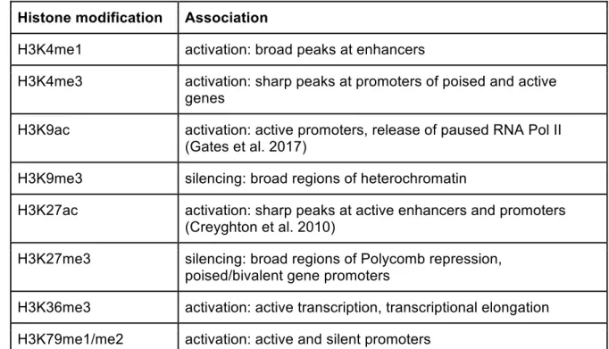
transcribed genes tend to have nucleosomes with high levels of trimethylation at lysine 36 of histone H3, abbreviated H3K36me3. Both promoters and active transcriptional enhancers are often marked with acetylation at lysine 27 of histone H3 (H3K27ac). Antibodies are available for many specific histone modifications, so that ChIP-seq can be used to measure these genome-wide. There are more than a hundred sites at which histones can be modified (Tan et al. 2011), but only a few of these have been studied in depth, summarised in Table 1.

Histone modification Association

H3K4me1 activation: broad peaks at enhancers

H3K4me3 activation: sharp peaks at promoters of poised and active genes

H3K9ac activation: active promoters, release of paused RNA Pol II (Gates et al. 2017)

H3K9me3 silencing: broad regions of heterochromatin

H3K27ac activation: sharp peaks at active enhancers and promoters (Creyghton et al. 2010)

H3K27me3 silencing: broad regions of Polycomb repression, poised/bivalent gene promoters

H3K36me3 activation: active transcription, transcriptional elongation H3K79me1/me2 activation: active and silent promoters

Table 1: Properties of widely studied histone modifications. Most are described in (Barski et al. 2007). Abbreviations are as follows: me1: mono-methylation; me2: di-methylation; me3: tri-methylation; ac: acetylation.

Histone modifications have contributed greatly to the annotation of regulatory DNA. They are one of the widely-used inputs for genome segmentation, in which a model attempts to

integrate multiple annotations to assign distinct states, such as enhancer, promoter, or transcriptional elongation, to each DNA segment across the genome (Ernst and Kellis 2012; Hoffman et al. 2012). Genome segmentation simplifies interpretation of the complex patterns of co-occurring histone modifications along the genome, which are often highly correlated amongst each other. However, because histones are present in nucleosomes with a periodicity along the DNA of ~150 - 200 bp, the resolution of regulatory information contained in histone modifications is also naturally limited to around 200 bp.

(24)

1.2.4 Chromatin accessibility

Regulatory regions of the genome have a DNA conformation that is open and accessible to transcription factor binding, whereas most other genomic regions have lower accessibility. A key advantage of measuring chromatin accessibility is that it is agnostic to the particular TFs that bind and open DNA at regulatory regions and promoters. Therefore, these regions can be identified in any cell type, without a need to assay each TF independently. In addition, using TF sequence motifs it is sometimes possible to predict the TFs that are bound at a regulatory region without directly measuring them. A method based on this idea, called centisnp, suggested that 97% of genetic variants in inferred TF binding footprints have no effect on chromatin accessibility (Moyerbrailean et al. 2016). Predictions from this method are used as one of the inputs the model that I describe in Chapter 3.

Until recently, chromatin accessibility was primarily measured by digesting native DNA with DNase I followed by sequencing, which found open chromatin covering about 1% of the genome. More recently, an alternative measure of chromatin accessibility based on integration of Tn5 transposase into native chromatin, known as ATAC-seq, has come into widespread use due to the simpler protocol and the ability to perform it with fewer cells (Buenrostro et al. 2013). Genetic variants influencing chromatin accessibility (caQTLs) can be identified with very modest sample sizes (< 100 individuals). While caQTLs do not directly indicate a target gene, the majority of caQTLs appear to be due to variants within the

chromatin accessibility peak that they regulate (Degner et al. 2012). This suggests that overlap between eQTLs and caQTLs can be a powerful method to localise causal eQTL variants.

1.2.5 Chromosomal conformation

Techniques such as Hi-C, which capture information about chromosomal interactions genome-wide, have shown that the genome is organized into topologically associating domains (TADs) of around 100 kb - 1 Mb, with the regulation of genes in different TADs insulated from each other (Dixon et al. 2012; Rao et al. 2014). One of the key factors determining chromosomal conformation is CTCF, a transcription factor with a particularly clear binding motif, which is found at TAD boundaries. Whereas TAD boundaries are largely conserved across cell types and across species, DNA contacts within TADs, such as

enhancer-promoter loops, are more dynamic and vary between cell types. Hi-C therefore has the potential to help in identifying causal regulatory variants by indicating the regulatory regions in contact with specific gene promoters.

(25)

Because Hi-C attempts to assay all pairwise interactions between DNA segments, achieving resolution of better than 25 kb requires a very large number of cells and deep sequencing (Rao et al. 2014). These requirements are reduced in promoter capture Hi-C, where an oligonucleotide pulldown enriches the Hi-C library for promoter-interacting regions before sequencing. Promoter capture Hi-C in 17 blood cell types by the BLUEPRINT consortium was used to prioritize 2,604 candidate genes for association with 31 GWAS traits (Javierre et al. 2016), although at each locus there were often a number of genes prioritized. Even when high resolution (<= 5 kb) is possible, it is difficult to detect significant interactions between DNA regions less than 25 kb apart, because nearby regions have a high rate of random collisions that are captured by the cross-linking used for Hi-C. However, it is clear from eQTL studies that the majority of causal regulatory variants are nearer than 25 kb from gene TSSes. This limitation reduces the utility of Hi-C data in localising causal regulatory variants.

1.3 iPSC-derived cellular models

While molecular traits can be measured in many cell types, technical limitations often make this difficult. Most assays require millions of cells, which are not always available from primary tissues, and this is particularly limiting for rare cell types. As a result, many of these assays have been performed on LCLs or cancer cell lines, even though these immortalized cells may not be good models for the relevant cell type. The use of induced pluripotent stem cells (iPSCs) provides a potential solution to both limiting cell numbers and poor cell type models. iPSCs can be expanded in vitro to the required number of cells, and then

differentiated in to specific cell types. Because iPSC technology is still quite new, it is important to understand the current state of the art.

1.3.1 Reprogramming somatic cells to pluripotency

In 2006, Takahashi and Yamanaka reported that somatic cells can be reprogrammed to pluripotency by the ectopic expression of just four transcription factors (Takahashi and Yamanaka 2006). This led to great excitement about the potential uses of these iPSCs for regenerative medicine, and in particular their advantages over embryonic stem cells (ESCs). IPSCs derived from a patient’s own cells could provide an unlimited supply of stem cells, which could be differentiated into desired cell types for cell-replacement therapies, and would be unlikely to face immune rejection. An early demonstration of the potential for this was provided by the Jaenisch research group, who derived dopaminergic neurons from reprogrammed mouse fibroblasts, and showed that implanting these into the brains of rat models of Parkinson’s disease led to functional integration and improved disease symptoms (Wernig et al. 2008). The development of such therapies for humans, however, depends

(26)

upon a thorough assessment of the safety and reliability of iPSC-based cells for specific applications, as well as the development of efficient protocols to derive specific cell types.

ESCs can differentiate into any cell type in the body; to be considered pluripotent, the same should be true of iPSCs. Although a number of reprogramming methods have now been developed, reprogramming is inefficient, and typically only up to 1% of somatic cells appear to attain pluripotency (Robinton and Daley 2012). As a result, iPS cell lines are grown from single-cell clones, and pluripotency is usually assessed by looking for molecular hallmarks, such as expression of genes OCT4, SOX2, and NANOG at levels comparable to ESCs. More robust validation of pluripotency can be obtained by showing that the cells can differentiate into the three embryonic germ layers in vitro. Even though iPSCs seem to be capable of differentiating into any cell type, a number of groups reported that individual cell lines showed more efficient differentiation to specific lineages (Kim et al. 2010). In particular, a concern is that iPSCs retain an epigenetic memory of the cell type they originated from, implying that reprogramming to pluripotency is generally incomplete (Bar-Nur et al. 2011; Polo et al. 2010). A problem with these comparisons was that the cell lines used were derived from different donors, and thereby had different genetic backgrounds. When Bock and colleagues used a quantitative differentiation assay as well as measuring DNA

methylation in 20 ESC and 12 iPSC lines, they found substantial variation among ESCs as well as iPSCs (Bock et al. 2011). In addition, global differences in gene expression are more significant in earlier passages of iPSCs, suggesting that pluripotency is gradually established over time (Polo et al. 2010).

More recently, cell banks of hundreds of human iPSC lines have been generated in a consistent manner by the NextGen consortium (Warren, Jaquish, and Cowan 2017) and the HIPSCI initiative (Kilpinen et al. 2017). These have revealed that donor genetic background contributes substantially to molecular variation in iPSCs. As well, improved protocols and characterisation of cell lines may help to overcome challenges related to the pluripotency and heterogeneity of iPSCs (D’Antonio et al. 2017; Panopoulos et al. 2017). For example, although it was was previously necessary to culture iPSCs on a “feeder” layer of mouse embryonic fibroblasts, new media with specific growth factors have enabled maintaining iPSCs without feeders, simplifying cell culture protocols.

A growing use of iPSCs is to differentiate them into specific cell types to model disease phenotypes in vitro. This is particularly valuable for rare and inaccessible cell types, which otherwise would be difficult to study. iPSC-derived cells can be used to discover cell

(27)

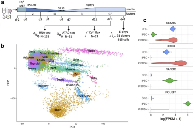
type-causal variants via gene editing with CRISPR-Cas9. These capabilities provide the motivation for the experiments described in Chapter 2. We differentiated iPSC lines from different donors in the HIPSCI project to pain-sensing sensory neurons, a cell type that would be difficult to study in vivo. By collecting multiple molecular phenotypes across a large panel of cell lines, the aim was to link common genetic variation with both molecular traits and electrophysiological traits of sensory neurons. In parallel with this experiment, a GWAS was conducted comparing more than 18,000 individuals with chronic pain to controls. The hope was that molecular QTLs from our study would inform interpretation of any GWAS loci associated with pain. Unfortunately, no genome-wide significant loci for pain were found. Despite this limitation, we found a number of QTL-GWAS overlaps that likely reflect neuronal functions more broadly. In addition, during the course of our work we came across a

challenge that has been noted in previous iPSC work, but which was particularly acute given the large number of differentiations in our study.

1.3.2 Heterogeneity and limited maturity of iPSC-derived cells

Differentiating iPSCs into defined cell types is a process that generally involves the addition of combinations of specific growth factors and media over a period of weeks, attempting to mimic endogenous developmental signals. A key challenge in using these as models is that although the resulting cells display characteristics of the desired cell type, they usually appear immature; this immaturity has been reported for multiple cell types, including neurons (Handel et al. 2016), hepatocytes (Dianat et al. 2013), cardiomyocytes (Veerman et al. 2015), and hematopoietic cell types (Smith et al. 2013). This may reflect in part the trade-off between experimental throughput and the time allowed for differentiation; however, it could also indicate that full maturation of cells requires a multicellular tissue environment that is absent in most culture systems (Passier, Orlova, and Mummery 2016).

A related but distinct challenge for iPSC-derived cell models is that differentiation tends to produce a mixture of cells, only a fraction of which express the expected marker genes. These differentiation outcomes can be highly variable between cell lines, and even across cultures of the same cell line. The nature of these “contaminating” cells is not generally known, but single-cell characterisation of cultures at multiple time points during

differentiation is beginning to shed light on factors that lead to this variability. Reconstructing the differentiation course of cells undergoing MyoD-mediated reprogramming to contractile myotubes suggested that cells can take alternative branches, with those that select incorrect branches ending in aberrant cell states (Cacchiarelli et al. 2017). For some cell types and applications, it is possible to sort differentiated cells to enrich for the desired outcome.

(28)

Another approach was described recently for neurons, where single cells were measured with patch clamp electrophysiology, followed by sequencing of the same single cells (Bardy et al. 2016). This approach enabled the researchers to link molecular cell states directly with functional features of the same cells.

Despite heterogeneity in iPSC differentiation, it has been possible to observe disease-relevant phenotypes for Mendelian diseases in derived cells. For example, iPSC-derived sensory neurons from patients with inherited erythromelalgia, which is due to

mutations in the sodium channel Nav1.7, showed greater spontaneous firing than those from control individuals, and this was reverted to normal with the addition of a Nav1.7-blocking drug (Cao et al. 2016). Similarly, iPSC-derived cardiomyocytes from individuals with long-QT syndrome showed prolonged action potentials, and this could be modulated by existing drugs used for long-QT syndrome (Itzhaki et al. 2011).

Heterogeneity is likely to be a greater problem when attempting to model the effects of complex trait-associated variants in vitro, due to their smaller effect sizes. Studies reported as part of the NextGen consortium have taken the first steps in this effort. Warren et al. recruited individuals homozygous for the major or minor genotypes (17 each) at the LDL-C associated variant rs12740374. They differentiated 68 iPSC lines from these individuals into hepatocytes and adipocytes, demonstrating that rs12740374 influenced SORT1 expression primarily in hepatocytes (Warren et al. 2017). Pashos et al. differentiated iPSCs from 91 healthy donors to hepatocyte-like cells, and used RNA-sequencing to map eQTLs. For four eQTLs that colocalized with GWAS associations for lipid traits, they used a massively parallel reporter assay to identify putative causal SNPs, followed by CRISPR/Cas9 genome editing to validate the candidate SNPs (Pashos et al. 2017). These impressive studies showed that using iPSC-derived cells to model complex trait associations is possible, but also revealed that doing so requires large samples sizes and very considerable effort.

1.4 Predicting variant functionality

Identifying causal variants for Mendelian or complex traits requires experimental validation. However, investigating the molecular effects of individual genetic variants is a laborious process that can usually only be done for a handful of variants at most. Computational approaches to prioritize variants to investigate are thus essential. The enormous growth in number and types of genomic data has fueled a growth in methods using these data to predict variant functionality and to fine-map GWAS associations. Predicting the functional

(29)

basic regulatory grammar that determines genome function. It is important to first clearly define what is meant by “functional”.

A widely held assumption, supported by evolutionary theory, is that most genetic variants are neutral, meaning that they have little effect on organismal fitness. This is consistent with the observation that a relatively small fraction of the genome (4-7%) has significant sequence conservation across mammals (Siepel et al. 2005; Davydov et al. 2010). Moreover, since selection depletes deleterious variants, the fraction of common variants with fitness effects is likely to be even lower. However, conservation differs from function. First, transcription factor binding sites generally have low conservation across species, despite having clear functional effects if disrupted (Doniger and Fay 2007). Second, variants may have “functional”

molecular effects without having organismal effects. Third, a functional variant may have a deleterious effect only late in life, and therefore have little effect on fitness and sequence conservation, even though it affects a trait. In this thesis, a functional variant is one with a molecular effect, regardless of whether that effect propagates to any other phenotype. Still, since neutral variants are unlikely to have effects on complex traits, functional variants are more likely to be causally related to complex traits.

1.4.1 Variant annotation

One way to stratify variants into classes that are more or less likely to have functional effects is to annotate them with available genomic features. A researcher can then manually assess the evidence for a given variant’s function using prior knowledge. Early annotation tools focused on identifying the effects of variants on protein-coding genes (Cingolani et al. 2012; McLaren et al. 2016). This is more technically challenging than it appears at first glance, and different tools often produce discordant annotations (D. J. McCarthy et al. 2014). Reasons for this include differences in gene annotations across reference databases, as well as the difficulty in determining the effects of variants on splicing. While these are essential tools, other annotations are important for predicting non-coding variant function.

The tool HaploReg (Ward and Kellis 2012) integrates a large number of genomic datasets, and reports a variant’s overlap with genes, enhancer and promoter marks, DNase

hypersensitive sites, protein binding sites, known eQTLs, and TF binding motifs. A useful feature is that it uses LD information to also annotate variants with r2 > 0.8 with the query variant. Interpreting the large number of overlaps is challenging, however. For GWAS associations it is typical to have dozens of variants in LD, a majority of which overlap some potentially relevant feature. RegulomeDB provides a heuristic solution to interpreting

(30)

overlapping annotations (Boyle et al. 2012): a variant is assigned to one of 14 handmade categories based on prior beliefs about the informativeness of each annotation. For example, a variant would receive a very high score if it alters a TF motif in a known TFBS, within a DNase hypersensitivity peak, and is also a known eQTL. A variant with fewer overlaps would receive a lower score depending on which annotations were absent.

1.4.2 Integrative approaches to score variant functionality

A general problem in predicting the functions of genetic variants is that informative annotations are correlated with each other. For example, while histone modifications H3K4me3 and H3K27ac are both enriched for eQTL variants, they frequently colocalise at gene promoters and transcribed enhancers, and so combining their independent

enrichments would overly prioritise variants where these annotations overlap. Methods have been developed which address this problem to predict variant functionality more rigorously.

Polyphen (Adzhubei et al. 2010) and SIFT (Kumar, Henikoff, and Ng 2009) are widely-used methods to predict the likelihood that a nonsynonymous protein-coding variant is deleterious. Both methods rely on the frequency of amino acid substitutions in homologous proteins, and Polyphen also considers protein structural features such as transmembrane domains and ligand-interacting regions. These methods are sometimes used as input to “meta-prediction” tools, which evaluate both protein-coding and non-coding variants genome-wide.

CADD applied machine learning to integrate many annotation sources, assigning a “deleteriousness” score to coding and non-coding variants (Kircher et al. 2014). Its inputs include Polyphen and SIFT, as well sequence conservation, and annotations from ENCODE such as DNase hypersensitivity, TFBS, and genome segmentations. CADD’s score is based on a support vector machine trained to distinguish common variants and human derived alleles from simulated variants, which are not present in the genome and so are presumed to have been depleted by selection. CADD has been widely used to prioritize variants in

studies of Mendelian disease. A particular strength is that it scores both coding and non-coding variants on the same scale, which enables evaluating both of these types of variation in relation to disease. However, CADD’s prediction performance is likely to be different for coding and non-coding variants, and CADD has been criticized for performing poorly on identifying functional variants in eQTL datasets (Gulko et al. 2015).

(31)

Troyanskaya 2015), and Basset (Kelley, Snoek, and Rinn 2016), and these are discussed in more detail in Chapter 3. Both the models implemented by these methods and the

annotations used as input differ, which makes it difficult to disentangle the factors influencing their relative performance. The general lack of a gold standard set of functional non-coding variants means that prediction performance can only be assessed relative to proxies, such as results from reporter assays. Although these scores of variant deleteriousness or functionality are clearly useful in some contexts, it is not clear how a variant’s score relates to its probability of influencing a particular trait. For complex traits, there is a need for methods that can be applied in a rigorous way to help in identifying causal variants.

1.5 Fine-mapping GWAS associations

Identifying causal variants at a GWAS locus is a key step towards deciphering the molecular mechanism behind the association. The first step towards this is fine-mapping - reducing the set of candidate variants from all those at the locus to a smaller set that is highly likely to contain the causal variant. Although most GWAS have used sparse genotyping to tag causal variants, a key assumption of fine-mapping is that the causal variant is among the variants considered. Therefore, samples within the study must either have whole genome

sequencing (the ideal case) or must have genotypes imputed using a reference panel from a genetically similar population of individuals. The set of candidate causal variants is often referred to as a credible set, which can be defined to have a specified probability of

containing the causal variant(s), given that particular assumptions are met. Commonly, 95% or 99% credible sets are reported. Approaches to fine-mapping can be roughly divided into those which are purely statistical, those which leverage additional data such as epigenomics and gene annotations, and experimental approaches.

1.5.1 Experimental evaluation of variants

The gold standard evidence to indicate that a specific variant has a causal effect is to experimentally replace the allele in a native cellular context. Following allelic replacement, cellular phenotypes such as gene expression can be assayed to determine whether the alleles differ in their activity on the same genetic background, with the assumption that alleles showing a molecular effect are likely to also causally influence the complex trait. Only recently have “genome editing” molecular tools such as CRISPR/Cas9 made this feasible, and the number of GWAS loci validated in this way remains small. Performing even a single such “knock-in” currently takes months at a minimum, and is difficult to perform in some cell types. A slightly lower standard of evidence is to use CRISPR/Cas9 to create small deletions overlapping a variant, which can show that the region covering the variant is

(32)

functional. When applying these approaches, it is critical to be highly confident that the causal variant is among the small number that can feasibly be tested.

A higher-throughput experimental alternative to genome editing is to use a reporter assay. Here, putative regulatory sequences, such as sequences surrounding highly ranked variants in an association study, are synthesized as oligonucleotides and inserted upstream of a reporter gene (e.g. green fluorescent protein (GFP) or luciferase) and transfected into cells. Sequences that regulate expression of the reporter gene will alter the measured level of GFP or luciferase. Reporter assays can also be done at scale. Tewhey and Sabetti used a massively parallel reporter assay (MPRA) to test 32,373 variants from 3,642 cis-eQTL loci for differential effect between alleles (Tewhey et al. 2016). Although this study focused on eQTLs rather than GWAS, the same approach could be used to test credible set variants from GWAS in cases where altered gene expression is the most likely mechanism. Even among eQTLs, MRPA only detected an expression-modulating effect of a genetic variant for ~9% of eQTLs tested, some of which will be false positives (Tewhey et al. 2016). It should be kept in mind that MPRA will only detect an effect for variants that alter gene transcription levels, i.e. enhancer or promoter variants, and not mechanisms that alter splicing or post-transcriptional regulation. Also, the effect that a variant has in a native cellular context may be unobservable or have a different direction of effect when tested in a reporter construct (Inoue et al. 2016). As a result, MPRA can be a useful complement to other fine-mapping approaches but does not obviate them.

1.5.2 Statistical fine-mapping

Early approaches to statistical fine-mapping, such as that used in the Wellcome Trust Case Control Consortium (Wellcome Trust Case Control Consortium et al. 2012), assumed that a single causal variant was present at an associated locus. A concern with this assumption is that when multiple causal variants do exist, the most strongly associated variants may be non-causal, due to being in LD with more than one causal variant. Leading methods developed more recently, such as CaviarBF (Chen et al. 2015), GUESSFM (Wallace et al. 2015), and FINEMAP (Benner et al. 2016), account for the possibility that multiple causal variants may explain the association signal. These approaches require testing different combinations of putatively causal variants, a task which quickly becomes computationally infeasible as more causal variants are allowed. GUESSFM and FINEMAP search a subspace of potential causal variant configurations that approximates the results obtained from examining all configurations. CaviarBF and FINEMAP require only summary statistics

(33)

genotypes are not available. To accomplish this, they depend upon an external reference panel of pairwise LD between variants, such as the 1000 genomes project or the Haplotype Reference Consortium. Importantly, the reference panel population’s ethnicity must be well-matched with that of the GWAS, otherwise the statistical fine-mapping may give spurious results. An additional drawback of purely statistical approaches is that when there are multiple variants in very high LD, they are nearly statistically indistinguishable.

1.5.3 Functional fine-mapping

Another set of methods incorporates functional genomic information to prioritize variants that have similar association statistics. This approach is supported by simulations showing that the size of the credible set can be reduced while retaining an equal probability of containing the causal variant (van de Bunt et al. 2015). Relevant annotations include overlap with gene bodies and proximity to gene TSSes, as well as the epigenetic traits discussed previously, such as chromatin accessibility, histone modifications, DNA methylation, and genome segmentation. Large-scale international consortia, such as ENCODE, Roadmap

Epigenomics (Roadmap Epigenomics Consortium et al. 2015), and FANTOM (FANTOM Consortium and the RIKEN PMI and CLST (DGT) et al. 2014), have collected epigenomic data across many cell lines and tissues.

The vast scale of epigenomic datasets makes their use for variant interpretation especially challenging because most variants overlap some molecular annotation. Furthermore, in the context of GWAS it is unclear how much weight to place on the statistical association for a given variant versus the annotations the variant overlaps. There has been rapid progress in computational methods that attempt to solve these two problems simultaneously. Fgwas (J. Pickrell 2013) learns each annotation's overall enrichment for statistically associated variants directly from GWAS summary statistics, controlling for LD between variants. In a Bayesian framework, each variant's prior probability of causality then depends on its annotations, and this is combined with its association statistic to determine a posterior probability that the variant causes the association in a region. Fgwas assumes that a single variant in each region causes the association. PAINTOR(Kichaev et al. 2014)uses a similar Bayesian approach, but allows for multiple causal variants, at the cost of running time that increases exponentially with the number of potential causal variants allowed. Because these

approaches rely on the signal from GWAS summary statistics, they are only likely to work well for highly powered GWAS where many associations contribute to the estimated

Using molecular QTLs to identify cell types and causal variants for complex traits