How Do Politicians Save? Buffer Stock
Management of Unemployment Insurance Finance
Steven Craig, Wided Hemissi, Satadru Mukherjee, and Bent E. Sørensen
∗Abstract
This paper studies how state governments manage the finances of their Un-employment Insurance (UI) programs. The operation of the UI programs is separate from states’ general budgets with clearly specified rules for saving (in a trust fund operated by the treasury) and spending, although spending includes a large discretionary component. Using a panel of US states we find that UI program spending and taxes are not described well by the PIH or by the Barro tax smoothing model. Instead, we find that states increase spending when their trust fund balance is high, and that trust fund balances seem to be clearly mean reverting. This pattern suggests that the data may be explained by a buffer stock model with forward looking but impatient politicians as suggested by Car-roll (1997) for consumers. We split UI benefits spending into a compulsory part (explained by unemployment) and a discretionary part. Considering taxes as income and discretionary benefits as consumption, we calibrate and simulate a version of Carroll’s buffer stock model. We find the simulation results of the buffer stock model match well our data, where politicians adjust policy to stay close to the target level of savings as shown by the simulation matching the co-variance condition where consumption and savings move with differences from the target level of savings.
1
INTRODUCTION
The objective of the research in this paper is to develop and test a model of how state governments adjust their stock of savings in response to economic cycles. We present a series of empirical tests using the US Unemployment Insurance (UI) system that sug-gest, for a case where the motivation for government savings accounts is clear, that a buffer stock model balancing impatience with risk aversion is an excellent description of government behavior. The recent economic downturn has spurred thinking about how governments might manage resources that could be used to smooth government con-sumption. Governments, however, are not the same as households, and consumption models cannot be seamlessly used to model governments. For example, the political economy/public choice perspective on government behavior would question whether in fact governments are able to save, even if they desired to do so, if politicians are systematically more impatient than residents.1 Further, the Ricardian view would
sug-gest that government savings or borrowing would be completely offset by households, in which case there would be no aggregate effect on savings or debt in the economy, and thus there would be no reason for the time path of government expenditures to fluctu-ate with the economy. Thus, to study how governments behave with respect to savings, we model state government management of UI savings accounts as an example of a government program that is explicitly designed to smooth economic fluctuations, and one for which there is likely to be private market failure so that systematic offsetting household behavior is unlikely.
The UI program in the US allows considerable latitude for individual states to adjust all four key program elements; benefit levels paid to unemployed individuals, the eligibility criteria for receipt by individuals, taxes levied on firms, and the level of UI trust fund savings. UI has the further advantage that each state maintains its system under a federal programmatic umbrella, which means the structure is similar between states despite significant policy differences. Further, UI addresses an actual market failure problem since insurance markets are faced with asymmetric information between buyers and sellers, which at least suggests a rationale for state governments to maintain an insurance-type reserve fund (Rothschild & Stiglitz, 1977). In the U.S. state governments maintain an explicit UI savings account called the UI Trust Fund,
1That is, if politicians are better off by spending any saved resources now, and they are not penalized for being
financed by an earmarked tax on firms, and make payments to unemployed workers only out of the UI Trust Fund. The institutional structure therefore makes feasible smoothing behavior over time, such as would be consistent with a Barro tax smooth-ing model or the Permanent Income Hypothesis (PIH). That is, the tax rate used to finance UI is not forced to instantaneously adjust to balance the state government budget as is true for general fund expenditures, instead states can theoretically follow tax smoothing or consumption smoothing strategies.2 An alternative possibility,
how-ever, is that state governments are impatient, and would want to spend the savings account immediately. Constraints on doing so include political opposition from raising taxes or cutting benefits during bad times, and the constraint imposed by the federal government on borrowing to fund UI trust fund shortfalls.
Our empirical work therefore uses a panel data set of the 50 US states from 1976-2010 to model how state governments manage their UI trust fund savings accounts. We first test whether the time path of state UI taxes follows a Barro tax smoothing model, or are consistent with a Permanent Income Hypothesis (PIH) type of consumer, and find using unit root tests both by state and as a panel that neither describes the data well.3 We then estimate a descriptive VAR model with UI taxes and benefits.
The resulting impulse response functions do not suggest temporary behavior to smooth consumption. Instead, we find that innovations in tax levels do not persist over time, and further that benefit increases are followed by increases in taxation. While we find that benefit payment increases exhibit a temporary component, we also find a considerable permanent component as well.
We estimate an ad hoc panel regression model to test how UI benefits and taxes respond to changes in trust fund balances. The estimation results suggest that state governments increase the generosity of UI benefits when trust fund savings balances are high. Increased UI expenditure is not the only path by which high savings balances are used, however, as we also find that state governments reduce UI taxes when savings balances are high. Finally, we find that when the state economy is strong UI benefits are increased, which of course also implies that benefits are reduced when the state economy is weak. This final result is the opposite of the nominal design of UI, where benefit expenditures are expected to increase in bad economic times. The results from
2That is, most state general fund expenditures are required to follow an annual balanced budget, see Poterba (1994). 3
the ad hoc model, however, are consistent with political UI managers that exhibit impatience by spending resources when they are available. On the other hand, the policy makers may also fear exhausting the UI trust fund balance in bad times, in which case the combination of these two influences suggests behavior consistent with the Carroll (1997) buffer stock model.
In a buffer stock model, an economic agent would maintain a precautionary savings account because of the fear of running out of money, or equivalently, of facing high costs from extreme policies to remedy a UI funding shortfall. If that same agent were impatient, defined as having an internal discount rate greater than the market rate of interest, then that agent would not allow the savings account to become too large. Jappelli, Padula, and Pistaferri (2008) have examined a buffer stock model using individual behavior, but find very little support using individual level data. We simulate their buffer stock model using parameters estimated from our data on state UI programs. We compare two statistical outcomes, a covariance condition which compares how both consumption and savings varies with deviations from target savings, and the actual level of target savings. In stark constrast to the failure of the buffer stock model for explaining individual behavior, we find that the behavior of state governments in managing their UI program appears quite consistent with buffer stock savings behavior. The conclusion which emerges is that UI program managers must be forward looking, and have a degree of impatience which is relatively well balanced with their degree of risk aversion. We therefore believe the buffer stock model offers a useful starting point for modelling how politicians manage the stock of savings for sub-national governments.
2
THE UNEMPLOYMENT INSURANCE SYSTEM,
AND DATA
The UI program consists of fifty individual programs, one per state, although within a federal government policy umbrella. States are allowed to vary both the eligibility rules, and benefit amounts, within certain parameters.4 If a person has been working
and loses their job due to “inadequate demand,” that person may receive benefits from
4http://www.ows.doleta.gov/unemploy/uifactsheet.asp is the US Labor Department website with facts about the
the state UI fund. Benefits are generally paid to equal about 60 percent of prior wages. States finance their UI program with an earmarked tax on employers. The tax rate varies between firms since it is partially experience rated, and it is typically only levied against the first $9,000 in annual wages.5 In this way the tax is essentially a lump sum
tax per employee. Recognizing that the share of the workforce that is unemployed is cyclical, states maintain a saving account, called a trust fund, for UI. The earmarked tax is paid into the UI trust fund while benefits are paid out of the UI trust fund. While in theory there is no interaction with the general fund of the state and thus no inter-play between various other taxes and expenditures, in fact there are a variety of taxes on firms. Thus state governments could raise or lower the level of UI taxation, and compensate with reverse changes of firm taxation in the General Fund, and thus move money from the UI trust fund to the general fund or vice versa.
States’ unemployment taxes are deposited with the US Treasury and states’ UI systems are able to borrow from the Treasury if their UI Trust Fund account goes to zero. The federal government pays interest on savings and charges state governments interest on loans; additionally there is a requirement for lending that state UI systems must be fundamentally solvent as determined by the Department of Labor (DOL).6
Thus, the primary impediment to state borrowing is in the form of the implicit regula-tion by the DOL. This suggests that the shadow price on borrowing for states could be extremely high and indeed, state borrowing from the Treasury is limited—this is im-portant because a crucial feature of the buffer-stock model is that agents are unable to borrow beyond a fixed limit.7 Our data suggests that no state goes beyond borrowing
5% of its covered wages.
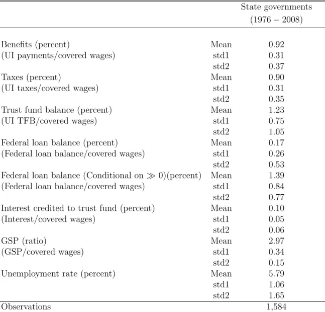
Table 1 presents the means of the panel data we use to examine state government management. Our panel of the 48 mainland U.S. states is from 1976-2008. The start date is dictated by the absence of state specific unemployment rates before 1976, al-though experimentation with other parts of the model suggest this restriction is not central to the results. The Unemployment Insurance program information is available from the DOL as all of the states run their UI program under the federal policy um-brella. The federal portion dictates that states have a similar framework of their tax
5The tax base varies between $7,000 and $16,000 in annual wages.
6In the environment of 2010-11 Congress has passed a waiver on interest payment on loans for all states.
and benefit structures, although they are free to make significant policy choices on the margin that cause significant policy differences between states (Craig and Palumbo, 1989). Also important is that the federal policy creates the UI Trust Fund for each state. The trust fund balances we use are reported as of the first of the year.
All of the dollar data in our project is deflated by the CPI. For the UI tax and benefit data, we normalize by covered wages, reflecting the insurance aspect of UI. UI does not necessarily cover all wages earned in the economy, as self employed workers are not generally covered (unless incorporated), and there are often caps on the total wages covered by UI (since benefits are a function of covered wages). Nonetheless, covered wages are over 90 percent of total wages.
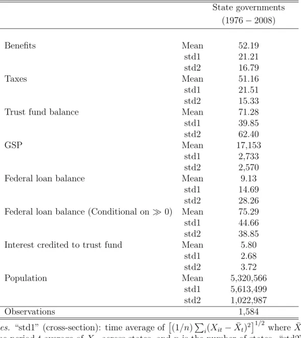
The means of our data are presented in Table 1. It shows that the UI program benefits and taxes are just under 1% of covered wages on average, although the share clearly fluctuates during business cycles. It also shows that the trust fund balance averages about 16 months of covered wages, so is substantial, although not large enough to forego taxation altogether for long. Interest earned by the trust fund averages 8% of the initial year balance for states. At the same time, about 12% of states are in debt to the federal government at any point in time. For those in debt, the debt levels are slightly above the average years’ reserves, so debt is important but is clearly not the modal behavior by states. Table 2 presents the dollars per capita of the variables in Table 1.
Craig and Palumbo (1989) address the motives underlying UI, and find that eligibil-ity varies substantially between states, and to a lessor extent so do benefits conditional on earned wages. They show that the variability is consistent with explicit policy choices by state governments, and in fact explain part of these UI choices using welfare policy choices. We therefore build our model to incorporate the “core” unemployment payments compared to the discretionary payments. Our definition of core payments is meant to include payments to UI recipients that would be eligible at all points in time. Discretionary payments are therefore those that states choose to make, or choose not to make, to people who are only eligible for UI in some circumstances at some points of time, but not other times. Examples would be UI payments to part-time workers, to workers with very short total work histories, to workers with a less well defined reason for separating from the employer, or to workers laid-off from a job after a very short period of work. Specifically, we run a regression on aggregate benefits as a function
of the unemployment rate, and we use the results of this regression to construct the expected value as our estimate of these ’core’ payments.8 We perform a similar
proce-dure for UI taxes, in that a portion of UI taxes go to fund the ’core’ UI payments, and the remainder is used to fund the discretionary UI payments.9
3
MODEL, TEST, AND SPECIFICATION OF
GOV-ERNMENT BEHAIVOR
The simplest model of forward looking government behavior is the Barro (1979) tax-smoothing model: a government facing an exogenous stream of expenditures and an increasing convex cost of period-by-period tax collection, will under certainty keep a constant tax rate such that the present value of taxes covers the present value of expenditure. Under uncertainty and quadratic costs, the government will display “cer-tainty equivalence” and choose the period t tax rate such that, if kept unchanged, it would have the same present value as the expected present value of expenditure. Barro showed that a simple testable implication is that the tax rate is a martingale (typically, if imprecisely, referred to as a random walk). Similarly, if utility of benefits are well approximated by a quadratic utility function and the discount rate is similar to the interest rate, expenditures will follow Hall (1978)’s celebrated version of the Perma-nent Income Hypothesis (PIH) and be well modeled as a martingale process. If tax rates are martingales, an autoregressive model fitted to tax rates should display a unit root. We therefore start out testing whether tax rates are approximately martingale by performing unit root tests. We also examine if expenditure rates are well fitted by autoregressive time series models with unit roots. If so, tax smoothing cannot be identified from unit roots, as pay-as-you-go behavior would deliver unit roots in tax rates for the simple reason that expenditures display unit roots. We next estimate a Vector AutoRegressive (VAR) model for expenditures and taxes and illustrate the intertemporal patterns in taxes and benefits, using both “rates” normalized by covered wages and by using Impulse Response Functions (IRF), although we do not interpret
8Specifically, we run a regression for each state to get a state-specific estimate of how UI beneifts vary with the
unemployment rate, and then average the estimates.
the error terms as structual innovations.10 The VAR model is a reduced form model
without structural interpretation, but it allows us to observe the adjustment pattern for both taxes and expenditures over time (Craig and Hoang, 2011).
There are good reasons to believe that governments may not act to perfectly smooth economic fluctuations. One reason is that politicians are under pressure to deliver cost effective services to their current taxpayers, so they are likely to reduce UI taxes to allow them room to increase other firm taxes, and generate a current service stream rather than build a UI trust fund. Similarly, if general fund revenues are low and there is political resistance to tax increases, a state government potentially may reap a political benefit from increases in UI benefits paid out, even if the UI trust fund is reduced. Thus the segmentation of the UI program from state fiscal policy in other policy dimensions is a political choice, rather than an institutional necessity. Further, there are other public good problems besides “smoothing,” and thus it may not be a surprise that several papers have rejected the PIH model for state governments and include a “rule of thumb” non-forward looking aspect (see, e.g., Dahlberg, Matz, and Tomas Lindstrom 1998), although this involves an unsatisfactory deviation from optimizing behavior.
The unit root tests we conduct, as well as the estimates of the VAR, strongly rejects these perfect foresight specifications. We therefore estimate a broader more explorative specification and, to preview, find evidence that states become more generous with benefits when the UI trust fund balance is high (although by implication this means benefits are less generous when the trust fund balance is low). We find equivalent behavior with taxation, that is that taxation tends to fall when the UI trust fund is flush, and tends to increase when it is low. Such a pattern is consistent with impatience (politicians with discount rates higher than interest rates would like to spend the saving in the trust fund). This view would be overly simplistic, however, because in general states do not exhaust their trust fund in its entirety, implying that politicians are forward looking to some extent, and so anticipate the loss of utility in future periods if the ability to pay UI benefits is exhausted. Despite these behaivoral justifications, the implication of this pattern of procyclical benefits and counter-cyclical taxation is the opposite of the usual automatic stabilizer label that is given to the UI program.
Models of impatient consumers that have an aversion to exhausting their savings
10Our preferred specification normalizes both taxes and expenditures by covered wages, although we show our
have been popularized by Carroll (1997) and Deaton (1991). A large of number of papers have attempted to test a key implication of the model: that “buffer stock” savings are larger when uncertainty is larger. The only direct test of buffer stock savings behavior, however, is a recent paper by Japelli, Pistaferri, and Padula (2008) that directly examines if consumers are prone to spend more if their savings exceed their (self-reported) desired stock of savings. We interpret (the discretionary part of) UI benefits as providing utility to politicians.11 To our knowledge, we provide the
first empirical evidence of buffer stock savings behavior by any agents, and believe our demonstration of buffer stock behavior by governments may hold important insights into policy designs that potentially aim at using governments to smooth economic fluctuations.12
4
BUFFER STOCK MODEL
Our empirical approach is to follow the approach of Japelli, Pistaferri, and Padula (2008) (JPP) to determine whether state governments exhibit the Carrol (1997) buffer stock behavior when managing their UI savings accounts. The JPP approach is un-usual, because they directly focus on the desired level of saving—i.e., the buffer stock. Our approach is similar, except that unlike their data our state government data does not contain a self reported desired buffer stock. Thus our objective is to use the JPP methodology to simulate the Carroll (1997) model, but then compare the resulting level of buffer stock savings to the level that is actually in our data. To construct the simulation problem, we develop the analog to individual consumption and income using our state UI data. The key factors in the model are the degree of risk aversion which tends to support a level of savings, and the rate of time discounting which tends to reduce the level of savings.
For our state government UI analog to the buffer-stock model, assume politicians get utility from the level of benefits paid, which we will model as consumption, C. Then the utility function can take the form of a state agent (consumer) maximizing:
11Likely due to higher benefit leading to higher chance of reelection, but we do not model the deeper meaning of
politicians’ “utility” in this paper.
12Part of this claim is because Japelli, Pistaferri, and Padula (2008) find no buffer stock behavior in the individual
Σ∞ t=1βt 1 1 +ρC 1−ρ t
where β is the time discount factor, Ct is consumption, and ρ > 0 is the coefficient
of relative risk aversion. The dynamic budget constraint facing the state government agent is
Wt+1 =R(Wt−Ct+Yt)
whereR is an interest rate factor assumed constant over time,Wt is non-human wealth
which in our model is the trust fund savings account, andYtis labor income (i.e., income
apart from interest income), which for us will be covered wages. In the original model agents are credit constrained and not allowed to borrow; i.e., Wt > 0, while in our
work we set a limit to possible borrowing. The funds available for consumption at the beginning of period t are Wt+Yt which Carroll (1997) denotes “cash-on-hand.” For
our UI model, income is tax receipts, so cash-on-hand equals the total of the trust fund at the beginning of the fiscal year plus tax receipts for the year.
Income is assumed exogenous and is typically modeled as the sum of a persistent (random walk) component, labeled permanent income, and a temporary (white noise shock) component:
Yt = PtVt , (1)
Pt = G PtNt . (2)
Pt is the permanent (unit root) component of income with log-normally distributed
innovationNt, where Var(ln(Nt)) =σN and E(ln(Nt)) = 0. Vt is the transitory (white
noise) component of income which is log-normally distributed with Var(ln(Nt)) = σV
and E(ln(Vt)) = 0.13 G is the deterministic growth rate of income.
Crucial features of the model are the lower bound on wealth (a maximum to borrow-ing) and a discount factor β which is lower than the interest rate factor. Impatience implies that the government desires to consume up-front and not build up savings, because the discount factor β is greater than the interest rate. Conversely, however, because zero consumption implies very high (infinite) dis-utility, the government will hedge against very low consumption by building a “buffer-stock” of saving, called here
13P
t is sometimes referred to as permanent income, although in the context of the PIH model, permanent income
the UI trust fund, to avoid running out of funds. Agents adjust their consumption and their target wealth one-to-one with movements in permanent income. We define all of the dollar variables (consumption, income, and cash on hand) relative to permanent income, and the normalized variables are all stationary. The model is solved by spec-ifying a parameter for risk aversion, a personal discount factor, and an interest rate (Carroll, 1997, JPP, 2008).
The “target buffer stock” is denote x∗, which is more precisely the target ratio of
cash-on-hand relative to permanent income. The innovation in Japelli, Padula, and Pistaferri (2008) is that they are able to directly make use of consumers’ (desired) buffer stock and examine if consumers whose “cash-on-hand” (savings plus current income) exceeds the buffer stock tend to increase consumption, thereby reducing deviation between cash-on-hand and the desired buffer stock of savings. Japelli, Padula, and Pistaferri (2008) test the model on their data based on the observation that agents whose cash-on-hand (relative to permanent income) exceeds the target will tend to decrease cash-on-hand in order to move toward the target. More precisely, they argue that the covariance of the cash-on-hand to target gap is negatively correlated with expected changes in cash at hand:
Cov{xt−x∗, Et(xt+1−xt)}<0.
Using the structure of the model, JPP rewrite this in terms of observable variables as
θ = Cov{xt−x∗, ct} Cov{xt−x∗, xt}
. (3)
We follow JPP and estimate the covariance ratio θ from our data and test if the buffer-stock model provides a reasonable fit to the data by comparing the empirically estimated value to the value ofθ implied by the model.
The covariance ratio satisfies a theoretical constraint (larger than 1−G/(Reσ2 N))
but in order to find exact numerical values forθas a function of preference and income parameters, one needs to simulate the model. We do so below for a range of values of the risk aversion parameter and the discount rate.
4.1
Mapping the UI Administrators’ decision problem into
the consumer model
We assume that the politicians who decide on the taxes and benefits derive utility from setting a high level of benefits. This utility would likely derive from generous benefits increasing the consumption of voters who then might be more likely to vote for the incumbent politicians. We do not attempt to sort out this mechanism but assumes that higher benefits deliver utility to politicians. However, part of benefits are clearly mandated by law to insure unemployed and we choose to consider the discretionary part of benefits as the equivalent of consumption in the buffer stock model.
We define a time period as two years but will also show some results for one- and three-year periods. The reason for choosing this interval is that governments—apart from rare exceptions—only change rules when a new budget is determined. This means that governments often can not react within a single year. Complicating matters, many states have two-year budgets. We do not have enough degrees of freedom to model states with different budgetary structures separately so we choose the two-year period as the best overall approximation. Regressions are done using non-overlapping two-year periods because it is hard to properly adjust standard errors for the serial dependence one would generate by using overlapping data.
We determine non-discretionary benefits by regressing UI benefits on the state un-employment rates. Residuals from this regression are assumed to be discretionary and we call these payments consumption.14 That is, we regress benefits on unemployment
for each state and find the average coefficient β. We then define non-discretionary benefits Cit =β∗(Uit−Ui.), where Uit is unemployment in state iin period t and Ui.
is average unemployment in statei. In the next iteration of this paper, we will add dis-cretionary taxes, with a negative sign, to consumption. More precisely, we perform the regression of benefit divided by covered wages (a unit free number) on unemployment and multiply the right hand side by covered wages when generatingC.
We define income as unemployment taxes minus non-discretionary benefits paid. In the next iteration of the paper, we will use the non-discretionary part of taxes instead of total taxes. We will approximate the non-discretionary part of tax with the fitted value from a regression of taxes on lags of non-discretionary benefits and covered wages.
14Craig and Palumbo (1998) show that UI benefits are heterogeneous by state due to state government preferences
We define permanent income as the three period moving average of income. In our preferred specification, using two-year periods, our moving average spans six years. As in the model, all variables are normalized by permanent income before we estimate the covariance ratio which is our (and JPP’s) main test of buffer-stock behavior.
Cash-on-hand is defined as the trust fund balance at the beginning of the period plus income as we define it plus 0.05*Covered Wages. This last term is added to allow for the possibility that state government UI funds may borrow from the federal government. There is a significant administrative shadow price of doing so, however, and the maximum we ever observe a state to borrow is slightly below 5% of the covered wages. We specify target hand as the three period moving average of cash-on-hand spanning six years.
Compared to the implementation of JPP, our data has the advantage of delivering exact savings balances, of having infinitely lived agents which implies that we do not have to separate buffer stocks from life-cycle savings, and of having precisely (albeit approximated) income where individual agents rarely report sources of “income” such as capital gains (the model assume lending at a constant interest rate), inheritance etc. JPP’s data directly measures consumption rather than our using a utility index on discretionary policy and they have access to self-reported target wealth observations.
This covariance ratio satisfies a theoretical constraint (larger than (1−G/(Reσ2 N)
but in order to find exact numerical values forθas a function of preference and income parameters, one needs to simulate the model. Because governments generally adjust finances slowly, we define each “period” for our mdoel as two years. This means we aggregate the data for each two year period and treat it as a single observation. We do not overlap the data, each period is consecutive (we do not use overlapping data because this usually leads to underestimated standard errors in regressions).
The definition of our variables to fit the JPP model starts with income. We define income as unemployment taxes minus non-discretionary benefits paid, where we deter-mine non-discretionary benefits by regressing UI benefits on the state unemployment rates. Residuals from this regression are therefore assumed to be discretionary, and we call these payments consumption. That is, we regress benefits on unemployment for each state and find the average coefficient β. We then define non-discretionary benefits as β∗(Uit−Ui.), whereUit is unemployment in state i in period t and Ui. is
the beginning of the period plus income minus consumption + 0.05*Covered Wages. This last term is added to allow for the possibility that state government UI funds may borrow from the federal government. There is a significant administrative shadow price of doing so, however, and the maximum we ever observe a state to borrow is slightly below 5% of the covered wages. We define permanent income as the three period moving average of income, which because each period is two years our moving average spans six years. Similarly, we specify target cash-on-hand as the three period moving average of cash-on-hand spanning six years.
5
RESULTS
Our results proceed in three steps. We first estimate a descriptive VAR with six lags to explore the relevance of the PIH or Barro tax smoothing models, and to provide descriptive statistics. These models are rather decisively rejected by the data. We then estimate an ad-hoc panel data model, in which we specify how either UI taxes or UI benefits paid respond to the level of the UI trust fund. We find that taxes generally fall as the trust fund balance grows, and that UI benefits grow as the trust fund balance grows. Both of these actions suggests buffer stock behavior, so our last step is to simulate Carroll’s (1997) model. The simulation gives us a target buffer stock savings level, which we find is close to the actual average levels in our data. Further, the simulation shows strong consistency with the covariance ratio condition derived in JPP, in which increases in the trust fund relative to the target is compared to increases in the trust fund relative to UI benefits. We find our data is also quite consistent with the covariance ratio condition.
5.1
VAR Regression Results
We explore the dynamic relation between UI taxes and benefits by estimating a VAR model with six lags of both UI taxes and benefits. We do not consider this a structural estimation because driving variables, such as wages and unemployment, are left out; however, VARs depict the dynamic relations between our two main variables succinctly. Moreover, one can directly get an impression of the validity of benchmark models such as the PIH and the Barro tax-smoothing model. In the PIH model, for example,
consumption (UI benefits) reacts instantly, not gradually, to changes in income (UI taxes). For the Barro tax-smoothing model, UI taxes react instantly to spending (UI benefits) shocks rather than gradually. In both cases, these reactions are because the shock communicates new information, which we expect the economic agent to instanteously use to adjust to the new permanent path. The other implication, of course, is that temporary shocks should cause little change.15
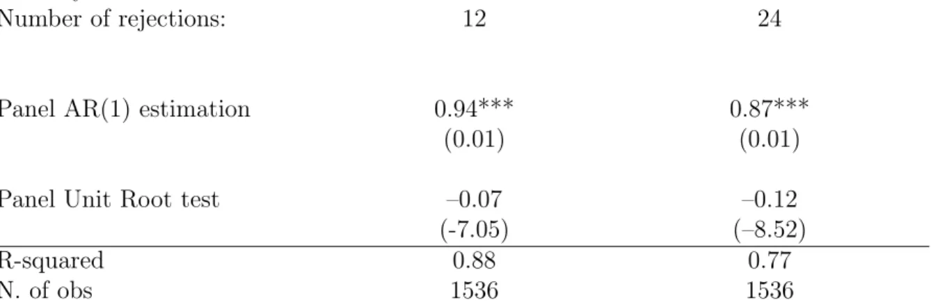
In Table 3 we report results of Dickey-Fuller unit root tests for log taxes and log benefits. UI benefits will be martingales, not rejecting unit roots, if benefits can be described as a consumption good for politicians with quadratic utility functions (see Hall, 1978 for more details). While unit roots tests are not very powerful for annual samples of only 38 years, we reject a unit root in benefits in 24 of 48 states at the 10 percent level of significance. Similarly for the Barro model, the unit root for taxes is rejected for only 12 states when each is tested separately.
Although these tests have low power, they suggest that 3/4 of the states potentially are following a tax smoothing path. Our interpretation, however, is that states engage in some tax smoothing, but not to the extent of following the Barro model closely.16
Pooled panel unit root tests, reported in the second row of Table 2, reject a unit root for UI taxes as well as benefits. The statistical rejection is slightly stronger for benefits than it is for taxes, but taxes are clearly not being systematically smoothed.
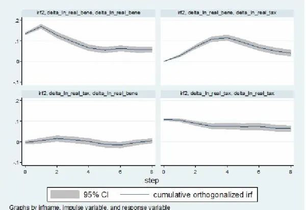
The coefficients from estimating the VAR are reported in Table 4 but the results are maybe more easily read from the graph of the Impulse Response Functions (IRFs) shown in Figure 1. Consider the regression of taxes on lagged benefits and taxes. Lagged benefits are significant with large coefficients of 0.20-0.30 for lags 1–4 clearly contradicting the Barro tax-smoothing model which implies that taxes are martingales for which all lags would be insignificant. Overall, taxes appears to adjust to benefits changes, likely in order to maintain a positive trust-fund balance. This endogenous aspect of taxes is ignored in the present implementation of the buffer-stock model be-low. Lagged taxes enters with negative coefficients indicating that UI-systems have something like a target for tax rates.17
15See Aiyagari, Marcet, Sargent, and Seppala (2002) for a more recent treatment, that nonetheless suggests these
interpretations hold, expecially in an environment where the government has a borrowing constraint as appears true for UI.
16State-level output and income are themselves unit root processes, see for example Asdrubali et al. (1996). 17This hypothesis may be rejected because the design of the UI program is that benefits should be paid out
counter-For the PIH model to explain how state governments manage their UI savings, we would expect that UI Benefits would be a martingale. In contrast, however, the results in Table 4 show that lagged benefits are very significant at explaining current benefits, indicating gradual adjustment to shocks. Conversely, the coefficient results of Table 4 do not show a consistent pattern of lagged taxes affecting current benefits. Several of the coefficients are insiginficant, and the signs switch for those that are significant. While not a formal model, and noting that there are no control variables, the general indication is that taxes are not adjusted by policy makers to provide benefits. The first lag of benefits indicates serial correlation in unemployment, but mean reversion takes is quite slow, at least 3 to 4 years (the standard error band is likely much too narrow for longer lags in the figure because they do not take into account the arbitrariness involves in selecting the correct number of lags).
5.2
Buffer Stock Regressions and Simulations
In this section we present two analyses. One is the ad hoc regression that estimates how UI benefits or taxes react to changes in the level of trust fund savings. Motivated by the results of this test, we then explore whether buffer stock behavior might explain state political UI choices. Specifically, we adapt our data to the JPP (2008) model of consumption and income, and compare the simulation using parameters estimated from our data to the UI data, and find that the buffer stock model seems to be a good fit.
Table 5 presents the results of an ad hoc regression, in which we separately model UI benefits or taxes as a function of, among other things, the level of the UI trust fund. Benefits are unsurprisingly found to react strongly to unemployment, and as well to the business cycle as captured by output growth. A recession dummy further captures the need for benefits in recessions. Benefits are found to rise with the level of GDP, which could include that politicians in wealthier states are more generous with unemployment benefits on average, or that benefits to the “marginally unemployed” rise during periods of high GDP. Interestingly, benefits are found to have a positive and
also important for the interpretation of the test of taxes. That is, if it is found that benefits follow a unit root, the test for UI taxes becomes uninformative since tax smoothing cannot be separated from simply budget balance. On the other hand, if the tests reject that UI benefits follow a unit root, then it is possible that our tests for UI taxes can differentiate whether taxes are designed by state governments to be smoothing taxes—i.e. whether UI taxes follow a unit root consistent with a smoothing governmental objective.
highly significant response to changes in the trust fund balance, a finding consistent with impatience. The tax equation finds that UI taxes rise in recessions, which might be surprising if we think about UI as an automatic stabilizer, and not so surprising if states are reacting to larger than usual UI expenditures. The regression further shows that taxes are raised when the trust fund balance is low, even after controlling for the state of the economy. While there is not an explicit model motivating this regression, the results are consistent with state government UI officials acting as buffer stock agents. That is, when funds are plentiful and the trust fund balance is high, politicians desire to spend money, including on UI benefits. On the other hand, when the business cycle is negative and the trust fund begins to run down, we find state policy makers respond to restore the trust fund, even if it means raising taxes during bad times. To formally test the buffer stock idea, we use the JPP (2008) simulation of the Carroll (1997) model with our UI data.
The simulation results of the buffer stock model are shown in Table 6. The pa-rameters we use in the simulation are derived from our panel data, where we treat UI benefits as consumption and UI taxes as income. The simulation is for 50 states with discount rates as indicated by β, and coefficients of risk aversion as indicated by ρ. The variance in transitory income is indicated byσV, as calculated from our data. The
objective is to find the resulting values of θ, which is the covariance ratio as indicated in equation (3). This ratio illustrates how the deviation from target wealth correlates with consumption, divided by the correlation between deviations from target wealth and the level of target wealth. We also use the simulation results to find the resulting value of x*, which is the target cash-on-hand to permanent income ratio. According to JPP, covariance ratios between about .4 and .8 are consistent with buffer stock be-havior, since it is consistent with extra consumption being correlated with buffer stock levels. The simulation results in Table 6 show that virtually all of the resulting co-variance ratios, θ, are within this range for a wide variety of parameterizations. When the results in Table 6 are compared to the actual data in Table 7 for the x* (target wealth, given here as the trust fund balance divided by covered wages), we see that the x* values generally fall within the range indicated by the data. We conclude from this that the buffer behavior implied by the buffer stock model is quite consistent with actual state government management of their UI systems.
6
SUMMARY AND CONCLUSION
The objective of this paper has been to examine how state governments manage the savings accounts that they accumulate to finance unemployment benefits. We believe this is the perfect institutional arrangement to examine government behavior with respect to savings, especially in the face of business cycle movements. The public good justification for state intervention seems well justified, thus private individual or firm actions are unlikely to obscure the objectives of state government officials. Further, UI is clearly the institution that is designed to respond to economic fluctuations.
We find that state government officials apparently are forward looking, but not to the extent that they would follow Barro’s advice to smooth taxes over time. Instead, we find that state governments alter both UI taxes and UI benefits in a manner that is consistent with impatient actors, but also actors that are risk averse. Indeed, we find using our simulations that state government behavior can be well characterized by a buffer stock model, suggesting relatively small fluctuations in the stock of savings around a target level.
One implication of our work is that at least in the case of UI, governments seem to be more forward looking and less impatient than the individuals in JPP’s data set, which might be inconsistent with the popular notion that government agents are “too present oriented.” The question which we have not yet addressed, but which would be crucial for understanding whether the UI institutional model could be extended more broadly to overall government expenditure, is the relative importance of specific institutional features for our behavioral findings. One implication of our findings, however, is that there is little government behavior that is “automatic,” as in automatic stabilizers, rather governments continually make choices and these choices depend on the objectives and tastes of policy makers, captured here by the trade-off between impatience and risk aversion.
References
[1] Asdrubali, Pierfederico, Bent E. Sorensen, and Oved Yosha, “Channels of Interstate Risk Sharing: United States 1963-1990," Quarterly Journal of Economics, 111:1081-1110, November, 1996. [2] Barro, Robert J., \On the Determination of the Public Debt." Journal of Political Economy, 87: 940-971, October 1979.
[3] Borge, Lars-Erik and Per Tovmo, \Myopic or Constrained by Balanced-Budget Rules? The Intertemporal Spending Behavior of Norwegian Local Governments," FinanzArchiv: Public Finance Analysis, 65 (2): 200-19, June 2009.
[4] Campbell, John Y. \Does Saving Anticipate Declining Labor Income? An Alternative Test of the Permanent Income Hypothesis," Econometrica, 55 (6): 1249-73, November, 1987.
[5] Carroll, Christopher D. \Buffer-Stock Saving and the Life Cycle/Permanent Income Hypothesis." Quarterly Journal of
Economics 112: 1-56, 1997.
[6] Chetty, Raj, and Emmanuel Saez, \Optimal Taxation and Social Insurance with Enodogenous Private Insurance," American Economic Journal: Economic Policy 2: 85-114, May, 2010.
[7] Craig, Steven G and Edward Hoang, \State Government Response to Income Fluctuations: Consumption, Insurance, and Capital
Expenditures," Regional Science and Urban Economics, forthcoming, 2011.
[8] Craig, Steven G and Michael G. Palumbo, \Policy Interaction in the Provision of Unemployment Insurance and Low-Income
Assistance by State Governments," Journal of Regional Science, 39 (2): 245-74, 1999.
[9] Dahlberg, Matz, and Tomas Lindstrom, \Are Local Governments Governed by Forward Looking Decision Makers?" Journal of Urban Economics, 44: 254-71, 1998.
[10] Deaton, Angus S. “Saving and Liquidity Constraints." Econometrica, 59: 1221-1248, 1991.
[11] Donovan, Colleen, \Direct democracy, term limits, and scal decisions in US municipalities," Conference paper, November 2009.
[12] Gruber, Jonathan, \The Consumption Smoothing Bene ts of Unemployment Insurance," American Economic Review, 87 (1):
192-205, March, 1997.
[13] Japelli, Tullio, Luigi Pistaferri, and Mario Padula, \A Direct Test of the Buffer-Stock Model of Saving," Journal of the European Economic Association, 6(6): 1186-1210, 2008.
[14] Nicholson, Walter, and Karen Needels, “Unemployment
Insurance: Strengthening the Relationship between Theory and Policy," Journal of Economic Perspectives, 20(3): 47-70, Summer, 2006.
[15] Rothschild, Michael and Joseph Stiglitz, \Equilibrium in Competitive Insurance Markets: An Essay on the Economics of Imperfect," Quarterly Journal of Economics, 90(4): 629-49, November,1976.
[16] Sorensen, Bent E., Lisa Wu, and Oved Yosha, \Output
Fluctuations and Fiscal policy:U.S. state and local governments 1978-1994," European Economic Review, 45: 1271-1310, 2001.
Table 1: Descriptive Statistics
State governments (1976−2008)
Benefits (percent) Mean 0.92
(UI payments/covered wages) std1 0.31
std2 0.37
Taxes (percent) Mean 0.90
(UI taxes/covered wages) std1 0.31
std2 0.35
Trust fund balance (percent) Mean 1.23
(UI TFB/covered wages) std1 0.75
std2 1.05
Federal loan balance (percent) Mean 0.17
(Federal loan balance/covered wages) std1 0.26
std2 0.53
Federal loan balance (Conditional onÀ 0)(percent) Mean 1.39
(Federal loan balance/covered wages) std1 0.84
std2 0.77
Interest credited to trust fund (percent) Mean 0.10
(Interest/covered wages) std1 0.05
std2 0.06
GSP (ratio) Mean 2.97
(GSP/covered wages) std1 0.34
std2 0.15
Unemployment rate (percent) Mean 5.79
std1 1.06
std2 1.65
Observations 1,584
Notes. “std1” (cross-section): time average of £(1/n)Pi(Xit−X¯t)2
¤1/2
where ¯Xt is
the period t average of Xit across states, and n is the number of states. “std2”
(time-series): average over iof £(1/T)Pt(Xit−X¯i)2
¤1/2
where ¯Xi is the time average
of Xit for state i, and T is the number of years in the sample. Benefits, Taxes, Trust
fund balance, GSP, Federal loan balance, Interest credited to trust fund are all normalized by Covered wages. Federal loan balance is positive for 12 percent of
Table 2: Descriptive Statistics (real dollars per capita with base (1982-1984)) State governments (1976−2008) Benefits Mean 52.19 std1 21.21 std2 16.79 Taxes Mean 51.16 std1 21.51 std2 15.33
Trust fund balance Mean 71.28
std1 39.85
std2 62.40
GSP Mean 17,153
std1 2,733
std2 2,570
Federal loan balance Mean 9.13
std1 14.69
std2 28.26
Federal loan balance (Conditional on À0) Mean 75.29
std1 44.66
std2 38.85
Interest credited to trust fund Mean 5.80
std1 2.68 std2 3.72 Population Mean 5,320,566 std1 5,613,499 std2 1,022,987 Observations 1,584
Notes. “std1” (cross-section): time average of £(1/n)Pi(Xit−X¯t)2
¤1/2
where ¯Xt is
the period t average of Xit across states, and n is the number of states. “std2”
(time-series): average over iof £(1/T)Pt(Xit−X¯i)2
¤1/2
where ¯Xi is the time average
of Xit for state i, and T is the number of years in the sample. Benefits, Taxes, Trust
fund balance, GSP, Federal loan balance, Interest credited to trust fund are all expressed in real per capita terms. Federal loan balance is positive for 12 percent of
Table 3: AR(1) Estimation
log(tax/covered wages) log(benefits/covered wages) State by state Unit Root Tests
Number of rejections: 12 24
Panel AR(1) estimation 0.94*** 0.87***
(0.01) (0.01)
Panel Unit Root test –0.07 –0.12
(-7.05) (–8.52)
R-squared 0.88 0.77
N. of obs 1536 1536
Notes. The first row reports number of rejections of unit roots in augmented
Dickey-Fuller tests. The second row reports the point estimates of the respective lagged variable in a standard panel AR(1) estimation with state fixed effects with standard errors in parenthesis. The last rows report test statistics and p-values from panel unit-root tests. *, ** and *** refer to the 10%, 5% and 1% significance level respectively
Table 4: VAR Estimation ∆(Taxes) ∆(Benefits) lagged ∆(Taxes): (t−1) -0.03 0.09* (0.03) (0.04) (t−2) -0.16*** 0.07 (0.03) (0.03) (t−3) -0.16*** -0.04 (0.03) (0.03) (t−4) -0.07** -0.00 (0.03) (0.03) (t−5) -0.07** -0.10** (0.03) (0.03) (t−6) 0.01 -0.00 (0.03) (0.03) (t−7) -0.04 0.04 (0.02) (0.03) lagged ∆(Benefits): (t−1) 0.21*** 0.27*** (0.02) (0.03) (t−2) 0.27*** -0.41*** (0.02) (0.03) (t−3) 0.30*** -0.08** (0.02) (0.03) (t−4) 0.20*** -0.31*** (0.02) (0.03) (t−5) 0.09*** -0.07* (0.02) (0.03) (t−6) 0.09*** -0.06* (0.02) (0.03) (t−7) 0.02 -0.13*** (0.02) (0.03) N. of obs 1175 1175
Notes: The table reports a VAR estimation for 1976-2008 period using the equation:
·
∆(ln(T axes/CoveredW ages)it
∆(ln(Benef its/CoveredW ages)it ¸ = 7 X k=1 · ak bk ck dk ¸ · ∆(ln(T axes/CoveredW ages)it−k
∆(ln(Benef its/CoveredW ages)it−k ¸
Table 5: Ad hoc Regressions of Benefits and Taxes
Benefits Taxes
Coef./Std. err. Coef./Std. err.
urates 0.03*** 0.01 (0.01) (0.01) log(GSP/Pop) 0.26** 0.16 (0.08) (0.09) ∆ log(GSP/Pop) -2.57*** -0.19 (0.27) (0.22)
log(trust fund bal at t-1) 0.47*** -0.80***
(0.10) (0.12)
∆ (log Trust fund bal) -0.28 -0.76*
(0.19) (0.35) Recession dummy 0.02* 0.04** (0.01) (0.02) lagged Benefits 0.68*** (0.03) lagged Taxes 0.80*** (0.02) R-squared 0.95 0.93 N. of obs 1536 1536
Notes: *, ** and *** refer to the 10%, 5% and 1% significance level respectively.
Table 6: The simulated covariance ratio and target wealth σV=0.1 σV=0.3 σV=0.5 β=0.9 β=0.94 β=0.9 β=0.94 β=0.9 β=0.94 ρ=0.5 θ = 0.86 θ=0.53 θ=0.69 θ=0.36 θ=0.54 θ=0.24 x∗=1.10 x∗=1.32 x∗=1.13 x∗=1.56 x∗=1.26 x∗=1.97 ρ=0.8 θ = 0.75 θ=0.27 θ=0.57 θ=0.21 θ=0.43 θ=0.17 x∗=1.15 x∗=1.72 x∗=1.26 x∗=2.03 x∗=1.45 x∗=2.61 ρ=1 θ = 0.66 NA θ=0.49 NA θ=0.38 NA x∗=1.24 x∗=1.37 x∗=1.61 ρ=1.4 θ = 0.43 NA θ=0.35 NA θ=0.26 NA x∗=1.51 x∗=1.69 x∗=2.04
Notes: The table reports the median simulated covariance ratioθand the median simulated target wealth to permanent income ratiox∗under alternative parameterization of a buffer stock
economy populated by50 individuals with same discount factorβliving for100periods. ρand
σV stand, respectively, for the coefficient of relative risk aversion and the standard deviation of
transitory income shocks. Simulations correspond to a standard deviation of permanent income shocksσN =0.3 and a probability of zero incomep =0.01. NAis reported in the cases where a
Table 7: IV regression of discretionary benefits on cash-on-hand
Benefits/ Covered wages
Diff=1
Estimated coefficient of cash-on-hand 0.40∗ (0.22)
Observations 1392
Diff=2
Start year=1977
Estimated coefficient of cash-on-hand 0.49∗∗∗
(0.12)
Observations 672
Diff=3
Start year=1978
Estimated coefficient of cash-on-hand 0.45∗∗∗
(0.06)
Observations 384
State and year fixed effects Yes
Notes: Standard errors in parentheses. For Diff=1 we treat each year as a period. For Diff=2 we treat two consecutive years to be a period. We sum taxes, benefits, covered wages, interest credited to the trust fund for two consecutive years be the value for a single period. For Diff=3 we treat three consecutive years to be a single period. We run an IV regression of discretionary benefits defined as [Benefits-β*(unemp-meanunemp)*covered wages] on cash-at-hand defined as [Trust fund balance+ .01 + taxes-β*(unemp-meanunemp)*covered wages]. We use the deviation between cash-on-hand and the target ratio of cash-at-hand as the instrument. We approximate the target cash-on-hand to be a 5 year moving average of cash-on- hand for Diff=1. We approximate the target cash-on-hand to be a 3 period moving average of cash-at-hand for Diff=2 and Diff=3 (i.e.; for Diff=2 we use the moving average of 3 periods of the 2 year sums). βis the between state mean ofβ generated from a state panel regression of benefits/covered wages on unemp. All variables are normalised by permanent income. Income is defined as [Taxes-β*(unemp-meanunemp)*coveredwages]. We define permanent income to be a 5 year moving average of income for Diff=1. For Diff=2 and Diff=3 we define permanent income to be a 3 period moving average of income. For Diff=2 the estimated coefficient of cash-at-hand is 0.43 if start year=1976. For Diff=3 the estimated coefficients of cash-on-hand are 0.48 and 0.49 respectively for start years 1976 and 1977. *, **, *** Significant at the 10 percent, 5 percent, and 1-percent level, resp.
Table 8: Cash-on-hand, income and ratio of cash-on-hand to permanent income
Variable Name mean std1 std2
Diff=1 (One year period)
Cash-on-hand (percent) 1.06 0.26 0.36 (Cash-on-hand/GSP) Income (percent) 0.31 0.12 0.11 (Income/GSP) Ratio 4.17 1.64 1.86 β 0.0019 0 0 Observations 1584
Diff=2 (Two year periods) Start year=1977 Cash-on-hand (percent) 0.85 0.16 0.17 (Cash-on-hand/GSP) Income (percent) 0.31 0.12 0.09 (Income/GSP) Ratio 3.26 1.02 0.91 β 0.0018 0 0 Observations 768
Diff=3 (Three year periods) Start year=1978 Cash-on-hand (percent) 0.77 0.14 0.12 (Cash-on-hand/GSP) Income (percent) 0.31 0.12 0.09 (Income/GSP) Ratio 2.86 0.82 0.62 β 0.0019 0 0 Observations 480
Notes: “std1” (cross-section): time average of£(1/n)Pi(Xit−X¯t)2¤1/2 where ¯Xt is the periodtaverage ofXit
across states, andnis the number of states. “std2” (time-series): average overi of£(1/T)Pt(Xit−X¯i)2 ¤1/2
where ¯
Xiis the time average ofXitfor statei, andT is the number of years in the sample. Diff=1 is the specification where
each year is treated as a period. Diff=2 is the specification where we treat two consecutive years to be a single period. We sum taxes, benefits, covered wages, GSP, interest credited to the trust fund for two consecutive years and treat that to be the value for a single period. Diff=3 is the specification where we treat three consecutive years to be a single period. Cash-on-hand is defined as [Trust fund balance + .01+ taxes-β*(unemp-meanunemp)*covered wages]. Income is defined as [Taxes-β*(unemp-meanunemp)*coveredwages]. βis the between state mean ofβgenerated from a state panel regression of benefits/covered wages on unemp. Cash-on-hand and Income are divided by GSP. Ratio is Cash-on-hand/ Permanent Income. We define permanent income to be a 5 year moving average of income for Diff=1. For Diff=2 and Diff=3 we define permanent income to be a 3 period moving average of income. For Diff=2 and Start year=1976, the means of cash-on-hand, income, ratio andβare 0.85, 0.31, 3.21 and 0.0019 respectively. For Diff=3 and Start year=1976, the means of cash-on-hand, income, ratio andβ are 0.78, 0.31, 2.90, 0.0018 respectively. For Diff=3 and Start year=1977, the means of cash-on-hand, income, ratio andβare 0.78, 0.31, 2.86 and 0.0018 respectively.
Figure 1: Impulse response function for taxes and benefit
Notes: Figure 1 displays the estimated impulse responses following a one stanadard deviation shock to benefits (upper panels) or taxes (lower panles).
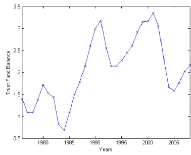
Figure 2: Simulated Target Balance Figure 3: Average Trust Fund Balance
Notes: Figure 2 displays the simulated amount of cash at hand relative to income for a buffer stock model with an agent having income growth of 4 percent, interest rate of 3 percent, risk aversion 2, and standard deviation of transitory and permanent shocks of 0.5 and 0.1, respectively. Figure 3 displays the year-by-year average over the U.S. states of (trust fund balance plus interest income plus tax) relative to income plus tax.