Reliability Assessment of a Power Grid with Customer Operated Chp Systems Using Monte Carlo Simulation

(1)

University of Massachusetts Amherst

ScholarWorks@UMass Amherst

Masters Theses 1911 - February 2014

2009

Reliability Assessment of a Power Grid with

Customer Operated Chp Systems Using Monte

Carlo Simulation

Lokesh Prakash Manohar University of Massachusetts Amherst

Follow this and additional works at:https://scholarworks.umass.edu/theses

Part of thePower and Energy Commons

This thesis is brought to you for free and open access by ScholarWorks@UMass Amherst. It has been accepted for inclusion in Masters Theses 1911 -February 2014 by an authorized administrator of ScholarWorks@UMass Amherst. For more information, please contact

[email protected].

Manohar, Lokesh Prakash, "Reliability Assessment of a Power Grid with Customer Operated Chp Systems Using Monte Carlo Simulation" (2009).Masters Theses 1911 - February 2014. 348.

(2)

RELIABILITY ASSESSMENT OF A POWER GRID WITH

CUSTOMER OPERATED CHP SYSTEMS USING MONTE

CARLO SIMULATION

A Thesis Presented by

LOKESH PRAKASH MANOHAR

Submitted to the Graduate School of the

University of Massachusetts Amherst in partial fulfillment of the requirements for the degree of

MASTER OF SCIENCE IN MECHANICAL ENGINEERING September 2009

(3)

RELIABILITY ASSESSMENT OF A POWER GRID WITH

CUSTOMER OPERATED CHP SYSTEMS USING MONTE

CARLO SIMULATION

A Thesis Presented by

LOKESH PRAKASH MANOHAR

Approved as to style and content by:

_________________________ Donald Fisher, Chair

________________________ Dragoljub Kosanovic, Member ________________________ Jon McGowan, Member

__________________________________________ Donald Fisher, Department Head

(4)

iii

ACKNOWLEDGMENTS

I would like to thank Dr. Beka Kosanovic for his mentoring, patience and support throughout my graduate program. Thanks to Dr. Donald Fisher and Dr. Jon G. McGowan for serving on my thesis committee.

I would like to acknowledge the help and assistance of all the fellow students and staff I have worked with in the Industrial Assessment Center. And thanks to my family for providing support and motivation.

(5)

iv ABSTRACT

RELIABILITY ASSESSMENT OF THE DISTRIBUTED NETWORK OF DISTRIBUTED GENERATION SYSTEMS USING MONTE CARLO SIMULATION

SEPTEMBER 2009

LOKESH PRAKASH MANOHAR, B.Tech., VELLORE INSTITUTE OF TECHNOLOGY UNIVERSITY

M.S., UNIVERSITY OF MASSACHUSETTS AMHERST Directed by: Dr. Dragoljub Kosanovic

This thesis presents a method for reliability assessment of a power grid with distributed generation providing support to the system. The distributed generation units considered for this assessment are Combined Heat and Power (CHP) units operated by

individual customers at their site. CHP refers to the simultaneous generation of useful electric and thermal energy. CHP systems have received more attention recently due to their high overall efficiency combined with decrease in costs and increase in reliability. A composite system adequacy assessment, which includes the two main components of the power grid viz., Generation and Distribution, is done using Monte Carlo simulation. The State Duration Sampling approach is used to obtain the operating history of the generation and the

distribution system components from which the reliability indices are calculated. The basic data and the topology used in the analysis are based on the Institution of Electrical and Electronics Engineers - Reliability Test System (IEEE-RTS) and distribution system for bus 2 of the IEEE-Reliability Busbar Test System (IEEE-RBTS). The reliability index Loss of

(6)

v

Energy Expectation (LOEE) is used to assess the overall system reliability and the index Average Energy Not Supplied (AENS) is used to assess the individual customer reliability. CHP reliability information was obtained from actual data for systems operating in New England and New York. The significance of the results obtained is discussed.

(7)

vi TABLE OF CONTENTS Page ACKNOWLEDGMENTS ... iii ABSTRACT... iv LIST OF TABLES ... ix

LIST OF FIGURES ... xii

CHAPTER 1.INTRODUCTION ... 1 1.1 Background ... 1 1.2 Research Motivation ... 4 1.3 Research Objectives ... 5 1.4 Methodology ... 5 2. RELIABILITY ASSESSMENT ... 7

2.1 Reliability Assessment Methods ... 7

2.2 Reliability Indices ... 11

2.3 Assessment Techniques... 14

2.3.1 Analytical Methods ... 15

2.3.2 Monte Carlo Simulations (MCS) ... 16

2.4 Reliability Test Systems and Data ... 20

3.SYSTEM MODELING ... 22

3.1 System Description ... 22

3.2 Load Modeling ... 25

(8)

vii

3.4 Distribution System Modeling ... 29

3.5 CHP Generation Modeling... 29

3.6 Reliability Assessment ... 32

3.6.1 Phase I – Before Installing CHP Units... 33

3.6.2 Phase II – After Installing CHP Units ... 33

4. DISTRIBUTION SYSTEM MODELING – BASIC TECHNIQUES... 36

4.1 Evaluation Techniques ... 36

4.2 Evaluation of the distribution system for busbar 2 of IEEE-RBTS ... 41

4.3 Distribution system modeling and simulation... 41

5. CASE STUDIES & RESULTS – PART I... 44

5.1 Common Aspects ... 44 5.2 Case Study 1... 45 5.3 Case Study 2... 47 5.4 Case Study 3... 50 5.5 Case Study 4... 56 5.6 Case Study 5... 60 6. CASE STUDY - 7... 63 7. CONCLUSION... 70 7.1 Summary ... 70 7.2 Future Work ... 72 APPENDICES ... 74

A. DETAILS OF IEEE-RELIABILITY TEST SYSTEM... 74

(9)

viii

C. CHP UNIT RELIABILITY DATA... 88

D. CALCULATION OF RELIABILITY PARAMETERS FOR THE DISTRIBUTION SYSTEM... 89

E. RESULTS OF CASE STUDY 3 ... 95

F. RESULTS OF CASE STUDY 4 ... 102

(10)

ix

LIST OF TABLES

Table Page

1.1 Typical Customer Unavailability Statistics ... 3

3.1: Customer Margin - Phase I ... 34

3.2: New Customer Margin – Phase II... 35

4.1: Component Data for the System shown in Fig. 4.1 ... 38

4.2: Load-Point Reliability Indices for the System of Fig. 4.1 ... 38

4.3: Reliability Indices with Lateral Protection ... 39

4.4: Reliability Indices with Disconnects and Lateral Protection... 40

4.5: Basic Reliability Indices for Load Points of Busbar 2 of IEEE-RBTS ... 42

5.1: Results of Case Study - 2 ... 50

5.2: Details of Case Study 3 – Phase II- Experiment 1 to 5... 51

5.3: Details of Case Study 3 – Phase II- Experiment 1 to 5... 52

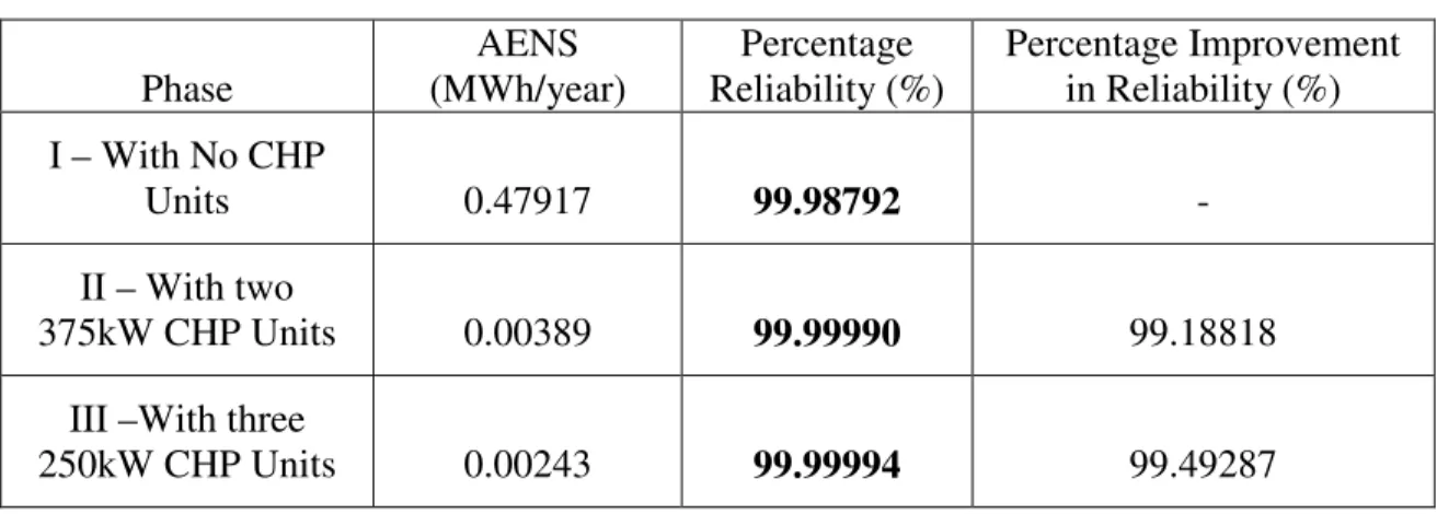
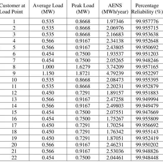
5.4: AENS and the Percentage Reliability for the 22 Customers in Case Study 3 Phase 1.... 53

5.5: New LOEE Index, Percentage Reliability for Phase II Case Study 3 ... 54

5.6: New AENS Index, Percentage Reliability for Customer 8 – Case Study 3... 56

5.7: AENS and the Percentage Reliability for the 22 Customers in Phase I - Case Study 4 .. 58

5.8: New LOEE Index, Percentage Reliability for Phase II Case Study 4 ... 59

5.9: New AENS Index, Percentage Reliability for Phase II Case Study 4 ... 59

5.10: Percentage Improvement in Reliability for the Customers Studied in Phase II - Case Study 4 ... 60

5.11: Reliability Parameters of the Distribution Line that Connects Customer 16 and Customer 22 to the busbar 2 ... 61

(11)

x

5.12: Results of Experiment 1 - Case Study 5 ... 61

5.13: Results of Experiment 2 - Case Study 5 ... 62

6.1: Reliability Parameters for the 600 kW and 190kW CHP Units ... 65

6.2: Details of the Experiments - Case Study 7 ... 67

6.3: Results for Experiments of Case Study 7 ... 68

6.4: LOEE Results for Experiments of Case Study 7 ... 68

A.1: IEEE – RTS Data for Centrally Controlled Generating Units ... 75

A.2: Weekly Peak Load in Percentage of Annual Peak... 75

A.3: Daily Peak Load in Percent of Weekly Peak ... 76

A.4: Weekly Peak Load in Percentage of Annual Peak... 76

B.1: Average and Peak Load of Customers at Various Load Points of the Distribution System... 78

B.2: Reliability Parameters of Distribution System Components ... 78

C.1: Reliability Parameters for CHP Units ... 88

D.1: Calculation of Reliability Parameters for the Distribution Lines ... 89

E.1: Case Study 3 Experiment 1 Results - 8% of the Load Supplied by CHP units... 95

E.2: Case Study 3 Experiment 2 Results – 15.5% of the Load Supplied by CHP units... 96

E.3: Case Study 3 Experiment 3 Results - 25% of the Load Supplied by CHP units... 97

E.7: Case Study 3 Experiment 7 Results – 100% of the Load Supplied by CHP units... 101

(12)

xi

F.2: Case Study 4 Experiment 2 Results - 15% of the Load Supplied by CHP units... 103 F.3: Case Study 4 Experiment 3 Results - 25% of the Load Supplied by CHP units... 104 F.4: Case Study 4 Experiment 4 Results - 50% of the Load Supplied by CHP units... 105

(13)

xii

LIST OF FIGURES

Figure Page

2.1: Power System – Hierarchical Levels ... 11

2.2: Two-Stage Generation Model... 15

2.3: Relationship between capacity, load and reserve ... 17

3.1: Flow Chart – Phase I... 24

3.2: Flow Chart – Phase II ... 25

3.3: Hourly Load Curve for Customer at Load Point 2 ... 26

3.4: Two-Stage Generation Model... 27

3.5: System Capacity Curve for One Year... 28

3.6: Sample Distribution Line Operational State Curve ... 29

3.7: Four-Stage System Model for CHP units ... 30

3.8: Sample CHP Unit Power Curve... 31

4.1: Simple 3-Load Point Radial System ... 37

4.2: System of Fig. 4.1 with Lateral Protection ... 39

4.3: Network of Fig. 4.1 with Disconnects and Lateral Protection... 40

4.4: Two-Stage Distribution Line Model... 42

5.1: Load Curve for the Customer(s) that is Studied in Case Study 1 ... 45

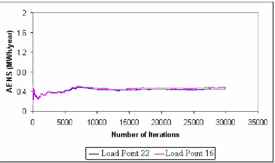
5.2: Monte Carlo Convergence of AENS for the Customer at Load Point 16 and Load Point 22... 46

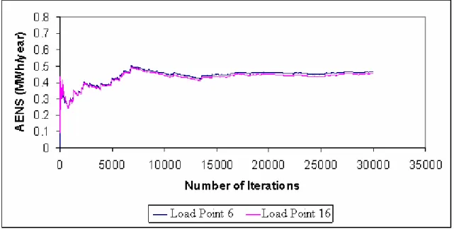
5.3: Monte Carlo Convergence of AENS for the Customer at Load Point 16 and Load Point 6 ... 47

(14)

xiii

5.4: Monte Carlo Convergence of AENS for Customer 22 with No CHP Units at Customer

Site ... 49

5.5: Comparison of Monte Carlo Convergence of AENS for Customer 22 with Two CHP Units and Three CHP Units ... 49

5.6: Monte Carlo Convergence of LOEE for Case Study 3 - Phase I... 53

5.7: Percentage Reliability, LOEE - Case Study 3 ... 55

5.8: Percentage Reliability, AENS, for Customer 8 – Case Study 3 ... 56

5.8: Monte Carlo Convergence of LOEE for Case Study 4 Phase I ... 57

6.1: Hourly Electric Demand Profile ... 64

6.2: Hourly Thermal Load Profile ... 64

6.3: Optimal Electric Power Output of the 600kW CHP Units ... 65

6.4: Hourly Electric Demand Profile for Customer 22 ... 66

6.5: Hourly Thermal Load Profile for Customer 22 ... 66

6.6: Optimal Electric Power Output of the 190 kW CHP Units ... 67

A.1: IEEE – Reliability Test System ... 74

B.1: Distribution System of Busbar 2 - IEEE–Reliability Busbar Test System ... 77

B.2: Hourly Load Profile of Customer 1 ... 79

(15)

xiv

(16)

1 CHAPTER 1

INTRODUCTION

1.1 Background

For many years electric distribution systems were designed and used only to deliver electrical energy to customers; no generation was present on the distribution systems or on the customer side of the meter [1]. However, due to major changes in the power markets and improvements in technology, generation capacities are increasingly being added to

distribution systems of power grid. These systems utilize both conventional and

unconventional sources of energy. Such systems may be operated by the customer or the utility itself. The process of generating electricity through systems that are located on the distribution network or at the customer site is known as Distributed Generation. The following may be cited as important reasons for the increased interest in DG systems [2]:

• availability of modular generating plant • ease of finding sites for smaller generators • deregulation or competition policy

• diversification of energy sources • national power requirement

• short construction times and lower capital costs of smaller plants

• generation may be sited closer to the load, which may reduce transmission costs Also, the liberalization of energy markets and the saturation of existing networks due to continuous growth in demand have provided a push for distributed generation [3]. An

(17)

2

new generation would be distributed [4]. In a distributed generation system, the generator may be operated by the utility or by the customer. In both the cases the operation of a DG unit may be considered random. However, in some cases the operation of a customer operated DG unit, though random, depends on the customer load. This is especially true in the case of a customer operated CHP units.

CHP stands for Combined Heat and Power. CHP refers to a subsection of DG units that simultaneously generate usable electric energy as well as thermal energy. It is also known as cogeneration. CHP units are primarily operated by customers that have

simultaneous need for both thermal energy and electric energy. By installing a CHP system designed to meet the thermal and electrical base loads of a facility, CHP can greatly increase the facility's operational efficiency and decrease energy costs. At the same time, CHP reduces the emission of greenhouse gases, which contribute to global climate change. More about CHP systems will be discussed in Chapters 3 and 6.

With rapid increase in demand and load on the existing networks distribution

generation is growing fast. As the distribution generation systems became widespread several issues including technology, economics and reliability need to be addressed. Reliability has been an important system issue and it has been incumbent on power system managers, designers, planners and operators to ensure that customers receive adequate and secure supplies within reasonable economic constraints. The primary aim of reliability studies has been to maximize the benefits to the society and reduce overall costs. Historically, reliability has been assessed using deterministic criteria, techniques and indices. Analytical

formulations have been used to evaluate the reliability of power system. However the

(18)

3

and random power flows, are stochastic in nature. This led to the evolution of reliability evaluation techniques using stochastic techniques. Stochastic techniques involve evaluating reliability using simulation methods, such as Monte Carlo simulation. Section 2.3 discusses the analytical and stochastic reliability evaluation techniques and the differences between the two.

The reliability evaluation of a power grid is a complex process. It requires a large amount of computer processing memory and time. Thus when the purpose of a study is to evaluate reliability of a particular subsystem it may not be of worth to model the entire system. Thus in order to simplify reliability evaluation process a power grid can be broken up into three levels viz., generation level, composite level (generation and transmission), and distribution system level. Studies can be conducted independently for each level to address various issues which may be specific to that level. Also studies performed at individual levels can be combined to evaluate the overall system reliability. Of the three levels, the distribution systems have received considerably less of the attention devoted to reliability modeling and evaluation [4]. One of the reasons is that the distribution system is relatively cheap and outages have a much localized effect. However, customer failure statistics of most utilities shows that the distribution system makes the greatest individual contribution to the

unavailability of supply to a customer. This is illustrated in Table 1.1. Table 1.1 Typical Customer Unavailability Statistics

Average unavailability per Contributor minutes % Generation/Trans mission 0.5 0.5 132 kV 2.3 2.4 66 kV and 33 kV 8.0 8.3 Distribution 86.0 88.8

(19)

4 1.2 Research Motivation

As outlined in the previous section, the reliability assessment of distribution networks has received considerably less attention. However, statistics such as that in Table 1.1

emphasize the need to be concerned with the reliability evaluation of distribution networks. Thus the primary purpose of this thesis is to demonstrate a method for reliability evaluation of distribution systems involving CHP generation systems.

The increase in demand for electricity has lead to saturation of existing electricity networks, congestion at network nodes and loss of energy experienced by the customers. While capacity addition by the utility is a traditional and common approach to address this problem, DG units, especially CHP units are being increasingly preferred due to their higher efficiency and faster implementation. However, at the same time, the reliability of CHP units is a concern. Individual CHP units are known to have poor reliability when compared to utility operated electricity generation units. In this light, it is necessary to evaluate and compare alternatives that are faster to implement, operationally more flexible in nature and, above all, more reliable.

Though CHP generation units have relatively poor reliability, their operation at a customer site has been found to improve the reliability of power supply to that customer. The adequacy assessment for power systems has been studied considerably in the literatures [5] and [6] and the adequacy assessment for distributed generation systems, with random input into the system, has been performed in [7] to find the Annual Unsupplied Load (AUL). However, the analyses presented in this thesis takes into consideration the measured real-time operating characteristics of individual customers and CHP units. Further, the analysis includes the effects of generation components as well as the distribution system which is the

(20)

5

major contributor to unreliability (the transmission components were considered to be 100% reliable).

1.3 Research Objectives

This thesis attempts to answer the following questions.

1) How can the distribution system of a power grid, with CHP units at various load points, be modeled realistically for the purpose of reliability assessment?

2) What is the quantitative effect to the overall system reliability and the individual customer reliability due to the CHP units operating at various customer load points?

3) What is the optimum location that a customer operated CHP system shall be installed in a distribution system?

1.4 Methodology

This study takes a stochastic approach to reliability evaluation. Monte Carlo simulation method is used to generate an operating history of various components of the power system based on the measured parameters of the components. The two main parameters are Mean Time To Failure (MTTF) and Mean Time To Repair (MTTR). The operating profiles of the components of the system, including the customer load profile, are superimposed to obtain an operation profile of the entire system from which the reliability indices are evaluated. The difference between the reliability indices obtained before and after the implementation of CHP units can serve as a guide to quantitatively understand the

significance of the difference made by CHP units to the existing system. Thus, the analysis is done in two phases. In the first phase, the adequacy assessment is performed on the system with the system power represented only by the power generated by the utility controlled

(21)

6

generation station. In the second phase, CHP units operating at various customer sites are included in the analysis. The methodology is elaborated in chapter 3 and 4.

For the purpose of analysis the Institution of Electrical and Electronics Engineers - Reliability Test System (IEEE RTS) and the IEEE-Reliability Test Busbar System (IEEE-RBTS) are used, as they represent a standardized model to enable different studies, which can then be validated by other results obtained from the systems. The unavailability of real data for system available capacity, reliability indices of various components of a power grid are also a driving factors in choosing the IEEE- Reliability Busbar Test System as the base system model for this analysis. Electric load profiles were also obtained from various customers, to enable realistic analysis of the system.

(22)

7 CHAPTER 2

RELIABILITY ASSESSMENT

Power systems have evolved over decades. Their primary emphasis has been on providing a reliable and economic supply of electrical energy to their customers. Spare and redundant capacities are inbuilt in order to ensure adequate and acceptable continuity of supply in the event of failures or forced outage of the plants, and the removal of facilities for regular schedule maintenance. Due to the improvements in distributed generation

technologies a significant amount of spare capacities are also being added on the customer sites. Distributed generation systems ensure adequate and acceptable continuity of supply in the event of failures in the generation, distribution and/or transmission systems [7]. The degree of redundancy has had to be commensurate with the requirement that the supply should be as economic as possible. It is necessary that maximum reliability is met within the set economic constraints. This optimization problem, which is to maximize reliability within given economic constraints has been widely recognized and understood.

2.1 Reliability Assessment Methods

Various methods have been developed to solve the aforementioned optimization problem. The methods can be broadly classified as: 1. Deterministic, 2. Probabilistic or Stochastic.

The typical criteria that are used by deterministic methods to evaluate the reliability of systems are:

1. Planning generation capacity – installed capacity equals maximum demand plus a fixed percentage of the expected maximum demand.

(23)

8

2. Operating capacity – spinning capacity equals expected load demand plus a reserve equal to one or more largest units.

3. Planning network capacity – construct a minimum number of circuits to a load group (generally known as an (n-1)(n-2) criterion depending on the amount of redundancy), the minimum number being dependent on the maximum demand of the group.

The deterministic methods are easy to use for simple systems but they do not and cannot account for the probabilistic or stochastic nature of system behavior such as frequency, duration and amount of failures.

In order to model and simulate the stochastic nature of the components of power systems probabilistic methods were developed. Also the general complexities of the power systems, which includes the large size of the systems, random nature of operation of the components, need to simulate variations arising due to weather conditions, etc, has played a major role in advancing reliability studies using probabilistic methods. Typical probabilistic aspects (as against the deterministic criteria mentioned above) are:

1. Forced outage rates of generating units are known to be a function of unit size and type and therefore a fixed percentage reserve cannot ensure a consistent risk.

2. The failure rate of an overhead line is a function of the length, design, location, and environment and therefore a consistent risk of supply interruption cannot be ensured by constructing a minimum number of circuits.

(24)

9

3. All planning and operating decisions are based on load forecasting techniques. These techniques cannot predict loads precisely and uncertainties exist in the forecasts.

Some probabilistic measures that are generally evaluated include: 1. system availability

2. estimated unsupplied energy 3. number of failure incidents 4. number of hours of interruption 5. excursions beyond set voltage limits 6. excursions beyond set frequency limits The above measures

1. identify weak area needing reinforcement or modifications 2. establish chronological trends in reliability performance

3. establish existing indices which serve as a guide for acceptable values in future reliability assessments

4. enable previous predictions to be compared with actual operating experience 5. monitor the response to system design changes

At this point, it is also necessary to understand the difference between absolute and relative measures. Absolute measures are useful in evaluating past performance. However, a high degree of confidence cannot be placed on absolute measures when they are used to predict future performance. On the other hand, relative measures are easier to interpret since the percentage improvement of a certain measure can be used to evaluate the before-and-after conditions. The indices used for reliability evaluation in this thesis are relative in that the

(25)

10

measures are evaluated and compared before and after the installation of CHP units at customer sites.

Power system reliability assessment can be divided into two basic concepts viz. system adequacy and system security. The concept of adequacy is generally considered to be the existence of sufficient facilities within the system to satisfy the customer demand. These facilities include those necessary to generate sufficient energy and the associated

transmission and distribution networks required to transport the energy to the actual consumer load points. Adequacy thus is considered to be associated with static conditions which do not include system disturbances.

Security, on the other hand, is considered to relate to the ability of the system to respond to disturbances arising within that system. Security is therefore associated with the response of the system to whatever disturbances they are subjected. These are considered to include conditions local and widespread effects and the loss of major generation and

transmission facilities. The security concept relates to the transient behavior of systems as they depart from one state and enter another state. The techniques presented in this thesis are concerned with adequacy assessment.

Modern power systems are immensely complex. Hence, in order to simplify various analyses that are performed on power systems, they are usually broken up into subsystems as shown in Figure 2.1. The analysis presented in this thesis is a hierarchical level 3 (HL 3). It involves modeling and simulation of generation and distribution facilities. The transmission facilities are considered to be 100% reliable.

(26)

11

Figure 2.1: Power System – Hierarchical Levels 2.2 Reliability Indices

The adequacy assessment of a power system involves evaluation of certain measures at one or more of the hierarchical levels. Each measure is concerned with a single reliability aspect or a combination of certain reliability aspects. Such aspects are system availability, estimated unsupplied energy, number of incidents, number of hours of interruption, etc. For example, some of the reliability measures are:

1. SAIFI – System Average Interruption Frequency Index

total number of customer interruptions SAIFI=

total number of customers served

2. SAIDI – System Average Interruption Duration Index

sum of customer interruption durations SAIDI=

total number of customers

(27)

12

total number of customer interruptions CAIFI=

total number of customers affected

4. CAIDI – Customer Average Interruption Duration Index sum of customer interruption durations CAIDI=

total number of customer interruptions 5. ASAI – Average Service Availability Index

customer hours of available service ASAI =

customer hours demanded

The measures that are evaluated in this thesis are the LOEE (MWh/yr) and the AENS (MWh/yr/customer) which are described below.

The Loss of Energy Expectation (LOEE) index incorporates the severity of

deficiencies in addition to their duration, and therefore the impact of energy shortfalls as well as their likelihood is evaluated. It is therefore often used for situations in which alternative energy replacement sources are being considered. This index is evaluated at the overall system level. Conceptually this index (LOEE) can be explained using the following mathematical expression.

∈

∑ i i

i S

LOEE = 8760 C p (2.1) Where i denotes the state of the system (whether the system is operational, has been shut down by the user or has failed), Ci is the loss of load for system state i,piis the

probability of system state i, and S is the set of all system states associated with the loss of load.

The Average Energy Not Supplied (AENS) index is used to evaluate reliability at the customer level (MWh/customer/year) is used. The choice of the index to be used for

(28)

13

for energy outage frequencies and durations was not available but load profiles for different customers within the system were, enabling the calculation of the total loss of energy over the year, the index AENS was used. Conceptually this index (AENS) can be explained using the following mathematical expression.

∈

∑i R i

ENS AENS=

N (2.2)

Where i denotes the point at which load is experienced (a load bus), ENS is the total Energy Not Supplied, Ni is the number of customers at load point i, and R is the set of load points in the system. The equations for calculating the above indices using probabilistic methods (Monte Carlo Simulation) are given in the Chapter 3.

During the initial years a number of techniques were developed for reliability

assessment. However, until 1979, there was no general agreement of either the system or the data that should be used to demonstrate or test proposed techniques. Consequently it was not easy, and often impossible to compare and/or substantiate the results obtained from various proposed methods. The IEEE Subcommittee recognized this problem on the Application of Probability Methods (APM), which, in 1979, published the IEEE-Reliability Test System (IEEE – RTS) [9]. This is a reasonably comprehensive system containing generation data, transmission data and load data. It is intended to provide a consistent and generally

acceptable set of data that can be used in generation system reliability evaluation. This has enabled results obtained by different people using different methods to be compared. The IEEE - RTS centre only on the data and results for the generation and transmission system: it does not include any information relating to distribution system. Thus, as an extension to IEEE - RTS, the IEEE - Reliability Busbar Test System (IEEE - RBTS) was published in 1991 [10]. The IEEE – RBTS outlines the topography of the distribution systems at busbar 2

(29)

14

and busbar 4 of the IEEE – RTS. It includes the main elements found in practical systems and thus serves as a common platform for evaluation of distribution systems.

Data collection and reliability evaluation should evolve together as both are very important aspects of system performance evaluation and one cannot be completely and realistically accomplished without the other. Data needs to be collected for two fundamental reasons; assessment of past performance and/or prediction of future system performance. In order to predict, it is essential to transform past experience into the required future prediction. Collection of data is therefore essential as it forms the input to relevant reliability models, techniques and equations. The data must be sufficiently comprehensive to ensure that the methods can be applied but restrictive enough to ensure that unnecessary data is not collected.

2.3 Assessment Techniques

In this section the actual methodology used in the two reliability assessment techniques, viz., analytical methods and stochastic methods, are discussed. Analytical techniques represent the system by analytical models and evaluate the indices from these models using mathematical solutions. Stochastic simulation involves real time simulation of the systems using the Monte Carlo simulation method. The stochastic simulation can be further classified as random or sequential. The random approach simulates the basic intervals of the system lifetime by choosing intervals randomly. The sequential approach simulates the basic intervals in chronological order. The analysis presented in this thesis involves Monte Carlo Simulation using the sequential approach.

(30)

15 2.3.1 Analytical Methods

Many analytical methods are based on the Calabrese approach [13] in which a Capacity Outage Probability Table (COPT) represents the generation model. The method is explained using an example of a two-stage model for generation as shown in Figure 2.2. 1/λ

UP DOWN 1/µ

Figure 2.2: Two-Stage Generation Model

Where λ = Expected failure rate (1/λ is the Mean Time to Failure - MTTF) and µ = Expected repair rate (1/µ is the Mean Time to Repair - MTTR)

The basic generating unit parameter used in adequacy evaluation is the unavailability, also known as the forced outage rate (FOR). The availability (A) and unavailability (U) are given by equations (2.3) and (2.4) respectively.

∑ ∑ ∑ λ MTTR DownTime Unavailability(FOR)=U= = = λ+µ MTTR+MTTF DownTime+ UpTime (2.3) ∑ ∑ ∑ µ MTTF UpTime Availability= A= = = λ+µ MTTR+MTTF DownTime+ UpTime (2.4)

A capacity outage probability table (COPT) is an array of the capacity levels and their probabilities of existence. The analytical method uses the recursive algorithm to form the COPT. The recursive algorithm for adding two state generating units is given by equation (2.5). This equation shows the cumulative probability of a certain capacity outage of X MW calculated after one unit of capacity C MW, with a forced outage rate U, is added

(31)

16

Where P’ (X) and P (X) are the cumulative probabilities of the capacity outage state of X MW before and after the unit of MW rating C is added. The generation model is then superimposed on the load model to calculate the desirable reliability index. The load model used depends upon the required reliability index. One common load model represents each day by the daily peak load, while another one represents the load using the individual hourly load values. If the daily peak loads are arranged in descending order, the formed cumulative load model is called the daily peak load variation curve. Arranging the hourly load values in descending order creates the load duration curve. This analysis uses the hourly peak load values for reliability index evaluation (load duration curve).

The relationship between load, capacity and reserve is shown in Figure 2.3. When the load duration curve is used, the shaded area Ek represents the energy that cannot be supplied in a capacity outage state k. The probable energy curtailed in this case is pkEk, where pk is the individual probability of the capacity outage state k. The Loss of Energy Expectation is then given by

∑

n k k k=1

LOEE = p E (2.6)

Where, n is the total number of capacity outage states.

The LOEE can be normalized using the total energy E under the load duration curve as shown in equation (2.7).

∑

n k k k=1 p E LOEE = E (2.7)

2.3.2 Monte Carlo Simulations (MCS)

The basic principle of MCS can be described as follows. The behavior pattern of n identical real systems operating in real time will all be different to varying degrees, including

(32)

17

the number of failures, the time between failures, the restoration times, etc. This is due to the random nature of processes involved. Therefore the behavior of a particular system could follow any of these behavior patterns.

Figure 2.3: Relationship between capacity, load and reserve

The simulation process is intended to examine and predict these real time behavioral patterns in simulated time, to estimate the expected or average values of the various

reliability parameters, and to obtain the probability distribution of each of the parameters. Some of the important aspects of Monte Carlo simulation are:

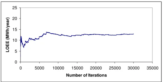
1. A large number of experiments are required to be performed in order to obtain a satisfactory result

2. The convergence toward the true value is obtained by performing a large number of experiments, though, the convergence may be slow.

(33)

18

of random numbers are generated. However, as long as the probability distribution function that defines the generation of random number remains the same, the true value to which the experiments converge is also the same.

The Monte Carlo simulation approach requires a large amount of computing time and storage in order to develop a good system model. However, the simulation technique is easy to apply and can be used to solve not only simple problems but also problems where direct analytical solutions may not exist.

One of the issues with Monte Carlo simulation method is the statistical noise. The basic idea of Monte Carlo simulation is to simulate the random transitioning of components from one state to another over the course of the experiment and to calculate the expectation value of the quantity of our interest in each experiment. Also, in the present thesis the customer loads for consecutive iterations are randomly varied within 5% of the observed using Monte Carlo method. It shall be noted that we start with a small set of information (generation system details, distribution system details, customer load details and CHP unit’s details) and conduct a large number of experiments (iterations) using the random values generated by the Monte Carlo method. While this is the primary advantage of the Monte Carlo method, it is also the disadvantage in that statistical errors are involved in the

calculations. The best way to minimize statistical noise is to estimate as many expectations of the quantity as possible by running a large number of experiments [17].

Simulation Process

Random number generation is the first step of a Monte Carlo simulation process. Usually a random number generator is used to generate uniformly distributed random number

(34)

19

U in the range 0 to 1. The present thesis employs the inbuilt function rand() in C++ to

generate the random numbers. The random numbers thus generated are converted into values representing a non-uniform probability distribution. Reliability studies of individual power system components have shown that the basic reliability indices of the components follow exponential distribution. In other words, the transition rate of a component from a state to another is exponential. Thus, say, λ_{is the Mean Time To Failure (MTTF) of a component in}

the system, the amount of time before the component fails (UP state) is given by equation (2.8). UP 1 T = ln U λ − (2.8) After the component has transitioned to the DOWN state it is necessary to calculate

the amount of time that the component shall reside in the DOWN state or the time remaining before it shall transition to the UP state. Equation (2.9) which is similar to equation (2.8) is used for this. The only difference is that the parameter Mean Time To Repair (MTTR), r is used in the equation.

DOWN 1

T = ln U

r

− (2.9) Thus, the random number generation process is used for simulating and estimating

the state durations of each component in the system. Hence this method is known as state duration sampling approach. The method is used to estimate the state durations or state history of generation units, distribution system components and CHP generation units. The system state history of each component in the system is superimposed along with the load curve of the customers to determine the reliability indices, the LOEE and AENS. This is dealt in greater detail in Chapter 3.

(35)

20 2.4 Reliability Test Systems and Data

IEEE – RTS

Meaningful reliability evaluation requires reasonable and acceptable data. These data are no always easy to obtain, and there is often a marked degree of uncertainty associated with the required input. Also an intended comparison between the results obtained from different reliability evaluation approaches can be made only if the approaches had used common power system configuration and basic reliability data. With these in mind, a reliability test system was developed in 1979, known as the IEEE Reliability Test System (RTS) [9]. The test system is a basic model that could be used to compare methods for reliability analysis of power systems. It includes generation and major transmission configuration and associated basic reliability indices, however, it does not include

distribution system configuration. The total installed capacity of the IEEE - RTS is 3,405 MW. The maximum peak load of the system is 2,850 MW. Appendix A summarizes all the relevant details of the IEEE RTS.

IEEE - RBTS

The IEEE – RTS has proved to be a valuable and consistent source for reliability studies involving generation and transmission studies. In order to provide a similar test bench for comparison of reliability evaluation methods involving distribution systems, the IEEE Reliability Busbar Test System (RBTS) was developed in 1991 [10]. In IEEE – RBTS distribution network designs were provided for two busbars from IEEE – RTS, viz., bus 2 and bus 4. It contains peak load and average load information of the customers in the buses. It also contains the basic reliability data of various components in the distribution network.

(36)

21

For the purpose of this thesis, the distribution system at bus 2 is selected for reliability evaluation. There are 22 load points in the distribution system of bus 2. The peak load of bus 2 is 20 MW and the average load is 12.29 MW. Each load point is connected to the main bus via 11/0.415 kV transformers, 11 kV breaker, 11 kV overhead line, 33/11 kV transformer, 33 kV breaker, 33 kV overhead line, 138/33 kV transformer and 138 kV breaker in that order. The configuration of the distribution system, customer load, and the basic reliability data for the components are summarized in Appendix B.

In order to estimate the reliability indices accurately hourly customer load profile information is desirable. Although, this can be generated using the customer peak and

average load data, the primary intention of this thesis is to evaluate reliability indices for real world customers. Hence, hourly load profiles were obtained from real world customers and from which 22 were chosen such that their average and peak loads match those given in IEEE - RBTS. The customer load profiles are shown in Table B.2 through Table B.23 of Appendix B. The sum of the customer load profiles gives the distribution system hourly load curve which is shown in Table B.1 of Appendix B.

(37)

22 CHAPTER 3

SYSTEM MODELING

3.1 System Description

Customers are supplied electricity via the distribution grid owned and controlled by certain utilities. This utility supplied power might not always be sufficient to meet the demand requirements of all the customers in its supply area. Some customers within the system can opt to install distributed generation units. This would mean that some of the customer load is invisible to the grid or the utility controlled substations when the DG units are in operation. However, when the DG units fail, the customers will rely on electric supply from the utility to meet their needs.

Combined Heat and Power (CHP) systems are the most commonly used Distributed Generation systems. The main difference between a CHP system and other DG technologies is that the CHP systems involve simultaneous generation of useful thermal and electric energy while other DG technologies involve generation of electricity only. A CHP system can have a total efficiency of over 80%, while the combination of electric energy obtained from a central power plant (with an efficiency of ~35%) and thermal energy obtained from an on-site boiler (with an efficiency of ~80%) has a total efficiency of approximately 50%. CHP systems are ideal for customers that have simultaneous electric and thermal load.

The CHP technologies usually consist of a heat engine that burns a fossil fuel

producing thermal energy. Part of the thermal energy is converted to mechanical energy in a prime mover, such as a turbine or reciprocating engine which in turn powers a generator. The rest of the thermal energy or the waste heat from the prime mover is directly used for thermal

(38)

23

energy requirements of the customer. Such requirements may be process heating or space conditioning. Various CHP system technologies include reciprocating engine-generator system, steam boiler-turbine-generator system, gas turbine-generator systems, and fuel cells.

This chapter explains the method to model a power generation and distribution system, which is then used to evaluate the impact that the CHP units have on the utility controlled system and also on the reliability of power supply to the customers. For the purpose of this thesis, the generation and distribution system under consideration is modeled from IEEE - RTS and IEEE - RBTS. The details of the IEEE - RTS and the IEEE - RBTS are given in Appendix A and B, respectively, and the systems are explained in Chapter 5.

The impact of CHP units on the system can be evaluated by conducting reliability analysis before and after the implementation of CHP units in the system. Thus, the reliability assessment is done in two phases; in phase I the reliability of the overall system and power supply to the customer are evaluated without any customer controlled CHP units operational in the system and in phase II the reliability is evaluated for the scenario wherein customer controlled CHP units are operating in the system. Figure 3.1 and 3.2 represents the flow of data and the modeling process in phase I and phase II respectively. In the following sections, the modeling process is elaborated.

(39)

24

Figure 3.1: Flow Chart – Phase I

Hourly Distribution Line Operational State Curve Distribution Modeling Generation Modeling Load Modeling Customers’ Load Details Hourly Load Curve Superimposition Hourly Power Curve Generation System Details Distribution System Components’ Details Customer Margin; LOEE; AENS

(40)

25

Figure 3.2: Flow Chart – Phase II 3.2 Load Modeling

The total load on the distribution system (Load system) and individual customer load (Load customer) for one year at least is required to conduct reliability test studies (one year’s worth of load data can take into consideration seasonal variation in load and other

irregularities.). A profile for the total hourly load on the distribution system is usually known to the utility for various load zones. This is a sum of all the customer loads on a particular

Generation Modeling Load Modeling Customers’ Load Details Distribution Modeling Distribution System Components’ Details Hourly Load Curve Superimposition

New Customer Margin; New LOEE; New AENS Generation System Details Hourly Power Curve CHP Units Modeling CHP Units’ Details Hourly CHP Power Curve Hourly Distribution Line Operational State Curve

(41)

26

distribution system. The hourly load for any customer is also available, usually monitored by the customers themselves or the utility. A sample hourly load curve for one of the customers is shown in Figure 3.3. This customer is assumed to be connected to the load point 2 (LP – 2) of the busbar 2 of the IEEE-RBTS. The load profiles for all the 22 customers in the busbar 2 of the IEEE-RBTS are given in Table B.2 through Table B.23 of Appendix B.

0.0 100.0 200.0 300.0 400.0 500.0 600.0 700.0 800.0 900.0 0 1000 2000 3000 4000 5000 6000 7000 8000 9000 Hours H o u rl y D e m a n d ( k W )

Figure 3.3: Hourly Load Curve for Customer at Load Point 2

For the purpose of this thesis several real time load data were obtained from a number of real world customers. From this pool of load profiles, 22 were chosen such that their peak load and average load are equal to the peak load and average load of the 22 load points in the busbar 2 of the IEEE-RBTS. These 22 load profiles are considered to be the load profile of the 22 load points and will be used for reliability assessment.

(42)

27

profile such that for each iteration (or year) the load profiles vary randomly by up to 5% from the collected load data. The result of load modeling is the customer hourly load curve and the sum of all customer load curves gives the distribution system hourly load curve.

3.3 Generation Modeling

The utility controlled substation is supplied with power by many utility-owned centralized generating units (could be coal, hydro, nuclear, oil, natural gas etc.). The working parameters for these generating units can also be obtained from the utility (Mean Time To Failure, Mean Time To Repair, and Scheduled Outage Factor for each unit). The present analysis uses details obtained from IEEE-RTS. These parameters are used to simulate the operating history for the power system.

These units have varying operating cycles and can be modeled as two stage systems as shown in Figure 3.4 (same as Figure 2.3). The UP state indicates that the unit is in its operating state and the DOWN state implies that the unit is inoperable due to a failure or a scheduled shut down. The transition from one stage to another is determined using the parameters Mean Time to Failure (MTTF – from UP to DOWN) and Mean Time to Repair (MTTR – from DOWN to UP). To model this two-stage system, the State Duration Sampling approach explained in section 2.3 is used.

MTTR

UP DOWN MTTF

Figure 3.4: Two-Stage Generation Model

Given that the transition of generation units from one state to another follows exponential distribution, the duration that a unit resides in a particular state is given by equations (2.8) and equation (2.9). The generation modeling step essentially involves

(43)

28

generating random numbers that are exponentially distributed, using the Monte Carlo simulation. Each random number thus generated is used in equations (2.8) and (2.9). The result of this step is a system state profile, i.e., the state of the unit and the amount of time it resides in the state before transitioning to the next state. Now generating capacities are assigned to the unit based on the state. During the UP state a full generation capacity is assigned to the unit and during the DOWN state the generating capacity of the unit is assigned to be zero. 0 500 1000 1500 2000 2500 3000 3500 4000 0 2000 4000 6000 8000 10000 Hours S y s te m C a pa c it y ( M W )

Figure 3.5: System Capacity Curve for One Year

The above process is repeated for all the units in the IEEE-RTS and summing up the assigned generating capacities for all the units results in the system power curve. The result of generation system modeling is the hourly power curve. A sample power curve for one year is shown in Figure 3.5.

(44)

29 3.4 Distribution System Modeling

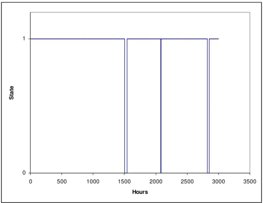
One of the main objectives of this thesis is to demonstrate a method to realistically model the distribution system of a power grid for the purpose of reliability evaluation. Hence, the modeling of a distribution system is explained in greater detail in chapter 4. The result of the distribution system modeling step is the distribution line operational state curve. A sample distribution line operational state curve is shown in Figure 3.6. In the figure, the UP state is represented by 1 and the DOWN state is represented by 0.

0 1 0 500 1000 1500 2000 2500 3000 3500 Hours S ta te

Figure 3.6: Sample Distribution Line Operational State Curve 3.5 CHP Generation Modeling

The CHP generation modeling step deals with two aspects. The first aspect is related to the modeling of the CHP generation units. The second aspect is related to the

(45)

30

The modeling of the CHP units is similar to the modeling of generation units that are operated by the utility, which is explained in section 3.3. The only difference is that the CHP units are modeled as four-stage systems, as shown in Figure 3.7, instead of the two-stage model that was used for utility operated generation units. It is assumed that at the beginning of the simulation, the CHP units are all in the UP state. The CHP unit can transition to the DOWN, DERATED or FAILED states from the UP state. The UP state indicates that the customer is operating the CHP unit at full generation capacity.

1 UP

2 DOWN 4 DERATED

3 FAILED

Figure 3.7: Four-Stage System Model for CHP units

The DOWN state is a “scheduled shut down” stage, i.e. the customer shuts down the CHP unit voluntarily. The DERATED stage indicates that the DG unit is operating at derated capacity, which is a certain percentage of the full generation capacity. The FAILED state indicates that the system has encountered an unscheduled shutdown. The transition from one state to another is determined by the basic reliability parameters: Mean Time To Failure, Mean Time To Repair and Schedule Outage Factor. The values of these parameters for the CHP units considered in this thesis are presented in Table C.1 of Appendix C. This

information is based on a study conducted at the Northeast CHP application center at the University of Massachusetts Amherst [16]

The electric power generated by the CHP unit follows the load requirement of the customer. Hence there might be more than one derated state present, or there might be no derated state present at all. To model the four-stage system, the State Duration Sampling

(46)

31

approach explained in section 2.4.2 is used. However, when the system is in the operational state, the electricity it generates will depend upon the customer load at that time, i.e. it might be running at full or derated capacity. The result of CHP generation simulation is the CHP power curve a sample of which is shown in Figure 3.8.

0 50 100 150 200 250 300 0 2000 4000 6000 8000 10000 Hour P o w e r (k W )

Figure 3.8: Sample CHP Unit Power Curve

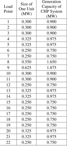
In order to perform an effective evaluation of the contribution of CHP units to the system and customer reliability it is necessary to determine the number, sizes and the location of CHP units that shall be operated at various customer sites. An important

conclusion of the work done by Tejal Kanitkar [14] is that the reliability of power supply to the customer is maximized when three CHP units operate at the customer site such that the combined capacity of the three CHP units is equal to the peak load of the customer. In the present thesis, this conclusion is first verified through a case study, and then extensively used in all the case studies.

(47)

32

The location of CHP units in the busbar 2 of the IEEE-RBTS is determined based on the following criteria. Consider the distribution system at the busbar 2 of the IEEE-RBTS. Given two customers with similar load profile, one nearest to the 33kV supply point (say, at load point 16) and the other farthest from the 33kV supply point (say at load point 22), it is first verified in case study 1 that the customer located farthest from the supply point

experiences the least reliability in power supply. It is inferred that this is due to the presence of additional components in the distribution line that connects the farthest customer to the supply point. Thus for the assumption that CHP units do improve the reliability of power supply to the customers, it is expected that the magnitude of improvement would be the largest if the CHP units are located at the customer site that is farthest from the supply point. Selecting a customer that is located farthest from the supply point as a potential site for the operation of CHP units might offer the best case scenario for reliability evaluation.

Based on this criterion CHP units are considered to operate at load point 22 for case studies 1, 2, and 5. The second criterion is based on the purpose of the case study. In case studies 1 and 5 which involve comparing the improvement in reliability for two customers load point 22 and load point 16 become the obvious choices. Case studies 3 and 4 are mainly concerned with the evaluation of overall system reliability when CHP units constitute a certain percentage of the total load. For these two case studies the load points, where CHP units shall be operated, are selected such that the sum of their average loads is 5%, 15%, 25%, and 50% of the total system load. The purpose, methodology and results of the case studies are elaborated in Chapter 5 and 6.

3.6 Reliability Assessment

(48)

33

above modeling steps. To evaluate the impact of CHP units on the system the reliability assessment is done in two phases - (A) before installing CHP units and (B) after installing CHP units

3.6.1 Phase I – Before Installing CHP Units

In Phase I, the Customer Margin is determined by superimposing the hourly load curve, the hourly system power curve of the utility owned generation units and the hourly operational system-state profile curve of the distribution line. Customer Margin is the Energy Not Supplied (ENS) to a customer at a given hour. Table 3.1 summarizes the different cases of the Customer Margin.

Using the Customer Margin, the system reliability index LOEE, and the customer reliability index AENS are calculated using the following equations.

( ) 1 N ENS customer i j i AENS j _N ∑ = = (3.1) ( ) 1 N ENS system i i LOEE N ∑ = = (3.2)

Where N denotes the number of iterations/years and ENScustomer denotes total Energy Not Supplied (MWh) to customer j in a given year. The sum of ENS of all the customers in the distribution system gives the ENSsystem. The value of ENS per iteration per customer is the sum of hourly Customer Margin (CM).

3.6.2 Phase II – After Installing CHP Units

Phase II includes all the simulations performed in Phase I plus the simulation of the CHP units that are considered to operate at various customer sites.

(49)

34

Table 3.1: Customer Margin - Phase I

Condition 1 Condition 2 Value of the Customer Margin State of the

distribution line is UP Zero Total power generated by

utility operated units is greater than or equal to

total system load State of the distribution line is DOWN

Portion of customer load not supplied

State of the

distribution line is UP

Portion of customer load not supplied Total power generated by

utility operated units is lesser than total system

load State of the

distribution line is DOWN

Portion of customer load not supplied

Thus, in Phase II, the New Customer Margin is determined by superimposing the hourly load curve, the hourly system power curve of the utility owned generation units, the hourly operational system-state profile curve of the distribution line and the hourly CHP units power curve. The New Customer Margin is then used to calculate the New AENS and the New LOEE using equations (3.1) and (3.2). Table 3.1 summarizes the different cases of the New Customer Margin.

By comparing the AENS and the LOEE, obtained in phase I, with the New AENS and the New LOEE, obtained in phase II, the contribution of CHP units to system reliability and the customer reliability can be evaluated.

(50)

35

Table 3.2: New Customer Margin – Phase II

Condition 1 Condition 2 Condition 3 Value of the Customer Margin

State of the distribution line is UP

CHP power is zero, greater than, lesser than or equal to the customer load Zero CHP power is greater than or equal to the customer load Zero Total power generated by utility operated units is greater than or equal to total system load

State of the distribution line is DOWN

CHP power is zero or lesser than the customer load

Portion of

customer load not supplied Power generated by utility units plus CHP power is greater than or equal to the customer load Zero State of the distribution line is UP Power generated

utility units plus CHP power is lesser than the customer load

Portion of

customer load not supplied CHP power is greater than or equal to the customer load Zero Total power generated by utility operated units is lesser than total system load

State of the distribution line is

DOWN CHP power is zero or lesser than or equal to the customer load

Portion of

customer load not supplied

(51)

36 CHAPTER 4

DISTRIBUTION SYSTEM MODELING – BASIC TECHNIQUES

This chapter is concerned with the basis evaluation techniques of simple radial

distribution systems. The technique is based on approximate equations for evaluating the rate and duration of outages that was first published in 1964-65 [15]. The techniques required to analyze a distribution system depend on the type of system being considered and the depth of analysis needed.

4.1 Evaluation Techniques

A radial distribution system consists of a set of series components, including lines, cables, disconnects (or isolators), busbars, etc. Henceforth, for simplicity, the term

“distribution line” would be used to collectively refer all the components that connect a load point to a supply point. A customer connected to any load point of such a system requires all components between himself and the supply point to be operating, in other words, the distribution line should be in UP state. The concept of series systems can be applied to these systems which results in the following equations for the three basic reliability parameters, viz., average failure rate, λ_s_{, average outage time, r}_s_{, and average annual outage time, U}_s_.

S i i

λ

=

∑

λ

(4.1) S i i i U =

_∑

λr (4.2) i i S i s S i i r U r λ λ λ = =

∑

(4.3)

(52)

37

In section 4.2, the method to obtain the operational history of the distribution line using the basic reliability indices, is explained.

Consider the radial system shown in Fig. 4.1. It is a simple system and any fault, single phase or otherwise will trip all the three phases.

Figure 4.1: Simple 3-Load Point Radial System

The assumed failure rates and repair times of each component are shown in Table 4.1. It shall be observed that the failure rate of lines and cables is proportional to their length.

Using, the above equations the load point reliability indices are calculated and are listed in Table 4.2. In this example, the reliability of each load point is identical. The

operating policy assumed for this system is not very realistic and additional features such as isolation, additional protection and transferable loads can be included. These features are discussed in the following sections.

(53)

38

Table 4.1: Component Data for the System shown in Fig. 4.1

Component

Length (km) Failure Rate, λ

(failures/year) Repair Time, r (hours)

1 2 0.2 4 2 1 0.1 4 3 3 0.3 4 4 2 0.2 4 a 1 0.2 2 b 3 0.6 2 c 2 0.4 2 d 1 0.2 2

Table 4.2: Load-Point Reliability Indices for the System of Fig. 4.1 Load Point Failure Rate, λ_L (failures/year) Repair Time, rL (hours) UL (hours/yr) A 2.2 2.73 6 B 2.2 2.73 6 C 2.2 2.73 6 D 2.2 2.73 6

4.1.1. Effect of lateral distributor protection

Additional protection is frequently used in practical distribution systems. One possibility in the case shown in Fig. 4.2 is to install fuse-gear at the tee-point in each lateral distributor. In this case a short circuit on a lateral distributor causes its appropriate fuse to blow; this causes disconnection of its load point until the failure is repaired but does not

(54)

39

affect or cause the disconnection of any other load point. The load point reliability indices that take into the consideration the effect of later distribution protection are shown in Table 4.3.

Figure 4.2: System of Fig. 4.1 with Lateral Protection

It shall be observed that the reliability indices are improved for all load points although the amount of improvement is different for each one.

Table 4.3: Reliability Indices with Lateral Protection Load Point Failure Rate, λ_L (failures/year) Repair Time, rL (hours) UL (hours/yr) A 1.0 3.6 3.6 B 1.4 3.14 4.4 C 1.2 3.33 4.0 D 1.0 3.6 3.6 4.1.2. Effect of disconnects

A second or alternative reinforcement or improvement scheme is the provision of disconnects or isolators at judicious point along the main feeder. These are generally not fault-breaking switched and therefore any short circuit on a feeder still causes the main breaker to operate. After the fault has been located, however, the relevant disconnect can be

(55)

40

opened and the breakers reclosed. This procedure allows restoration of all load points

between supply point and the point of isolation before the repair process has been completed. Let points of isolation be installed in the previous system as shown in Fig. 4.3 and let the total isolation and switching be 0.5 hour.

Figure 4.3: Network of Fig. 4.1 with Disconnects and Lateral Protection

The reliability indices for the four load points are now modified to those shown in Table 4.4.

Table 4.4: Reliability Indices with Disconnects and Lateral Protection Load

Point

λ_L

(failures/year) rL (hours) UL (hours/yr)

A 1.0 1.5 1.5

B 1.4 1.89 2.65

C 1.2 2.75 3.3

D 1.0 3.6 3.6

In the examples of section 4.1.1 and 4.1.2, it is assumed that the lateral protections and disconnects are 100% reliable.

(56)

41

4.2 Evaluation of the distribution system for busbar 2 of IEEE-RBTS

For the distribution system considered in this thesis, the evaluation technique includes the reliability of the following components: 33kV supply feeders, 11kV feeders,

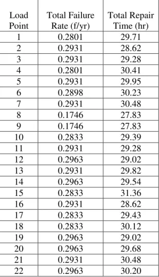
transformers, breakers, busbars, and lines. The lateral protection and disconnects are assumed to be 100% reliable. The system is considered to be a simple radial network. The failure rates and repair times for various components of the distribution system that connects each load point to the supply point is given in Table B.2 of Appendix B. Using the basic reliability indices of various components and the method explained in section 4.1.2 the basic reliability indices for each distribution line is calculated. Remember that a distribution line is used to refer all the components that connect the load point to the supply point. The reliability

parameters, Failure Rate (inverse of MTTF) and Repair Time (MTTR), for the 22 load points (distribution lines) are listed in Table 4.5. The calculations used to evaluate the reliability parameters are shown in Table D.1 of Appendix D.

4.3 Distribution system modeling and simulation

The modeling method is based on the treatment of a distribution line as a two state system: UP state and DOWN state. The UP state indicates that the distribution line is

operational and thus the load point is connected to the supply point. In other words, UP state indicates that all the components connecting the load point to a supply point is operational. The DOWN state implies that one of the components in the distribution line has failed and thus the load point is not connected to the supply point.

(57)

42

Table 4.5: Basic Reliability Indices for Load Points of Busbar 2 of IEEE-RBTS Load Point Total Failure Rate (f/yr) Total Repair Time (hr) 1 0.2801 29.71 2 0.2931 28.62 3 0.2931 29.28 4 0.2801 30.41 5 0.2931 29.95 6 0.2898 30.23 7 0.2931 30.48 8 0.1746 27.83 9 0.1746 27.83 10 0.2833 29.39 11 0.2931 29.28 12 0.2963 29.02 13 0.2931 29.82 14 0.2963 29.54 15 0.2833 31.36 16 0.2931 28.62 17 0.2833 29.43 18 0.2833 30.12 19 0.2963 29.02 20 0.2963 29.68 21 0.2931 30.48 22 0.2963 30.20

The transition from one stage to another is determined using the parameters Mean Time to Failure, (MTTF – from UP to DOWN) and Mean Time to Repair (MTTR – from DOWN to UP).

MTTR

UP DOWN MTTF

Figure 4.4: Two-Stage Distribution Line Model

The MTTF is the product of the inverse of failure rate and the number of hours being considered per iteration, in this case, 8,736 hours. The MTTR is the repair rate. At the start of