ISSN 1440-771X
Australia
Department of Econometrics and Business Statistics
http://www.buseco.monash.edu.au/depts/ebs/pubs/wpapers/
September 2011
Working Paper 20/11
A New Test in Parametric Linear Models against
Nonparametric Autoregressive Errors
A New Test in Parametric Linear Models
against Nonparametric Autoregressive Errors
By Jiti Gao1 and Maxwell King
The University of Adelaide and Monash University
Abstract: This paper considers a class of parametric models with nonparametric autore-gressive errors. A new test is proposed and studied to deal with the parametric specification of the nonparametric autoregressive errors with either stationarity or nonstationarity. Such a test procedure can initially avoid misspecification through the need to parametrically specify the form of the errors. In other words, we propose estimating the form of the errors and test-ing for stationarity or nonstationarity simultaneously. We establish asymptotic distributions of the proposed test. Both the setting and the results differ from earlier work on testing for unit roots in parametric time series regression. We provide both simulated and real–data examples to show that the proposed nonparametric unit–root test works in practice.
Key words: Autoregressive process; nonlinear time series; nonparametric method; random walk; semiparametric model; unit root test.
JEL Classification: C12, C14, C22
1Jiti Gao, Department of Econometrics and Business Statistics, Monash University, Caulfield East Victoria 3145, Australia. Email: [email protected].
1. Introduction
Consider a parametric linear model of the form
Yt =Xtτβ+vt, t= 1,2,· · · , T, (1.1)
where T is the sample size of the time series data{Yt : 1≤t ≤T}, {Xt}is a vector of
known deterministic functions, β = (β1,· · · , βp)τ is a vector of unknown parameters,
{vt} is a sequence of time series residuals. Existing studies mainly discuss tests for
the case where {vt} satisfies the first–order autoregressive (AR(1)) model of the form
vt =ρvt−1+ut with {ut} being a sequence of independent and identically distributed
(i.i.d.) errors. Discussion about tests for|ρ|<1 may be found in the survey papers by King (1987), King and Wu (1997) and King (2001).
For the case ofρ= 1, there has been much interest in both theoretical and empirical analysis of economic and financial time series with unit roots during the past three
decades or so. Various tests for unit roots have been proposed and studied both
theoretically and empirically. Models and methods used have been based initially
on parametric linear autoregressive moving average representations with or without trend components. Existing studies may be found in the survey paper by Phillips and Xiao (1998). Other studies include Dickey and Fuller (1979, 1981), Evans and Savin (1981, 1984), Phillips (1987), Phillips and Perron (1988), Dufour and King (1991), Kwiatkowski et al(1992), Phillips (1997), Lobato and Robinson (1998), and Robinson (2003).
As pointed out in the literature (Vogelsang 1998; Zheng and Basher 1999), there are cases where there is no priori knowledge about either the form of the residuals or whether the residuals are I(0) or I(1). This motives us to consider using a nonpara-metric autoregressive error model of the form
vt=g(vt−1) +ut, t= 1,2,· · · , T, (1.2)
where g(·) is an unknown function defined over R1 = (−∞,∞), {ut} is a sequence of
stationary errors with mean zero and finite variance σ2
u =E[u21], {vt : t ≥1} is also a
sequence of errors with E[vt] = 0, andv0 is an initial value. Note thatv0 can be either
a given initial value or any OP(1) random variable. We however set v0 = 0 to avoid
some unnecessary complications in exposition.
Combining model (1.2) into model (1.1) produces a semiparametric time series model of the form
Existing studies (see, for example, Masry and Tjøstheim 1995) already discuss the case where β ≡0 and {vt} is strictly stationary when certain technical conditions are
imposed on the form of g(·). Meanwhile, various existing studies (see, for example, Koul and Stute 1999; Gao 2007 and the references therein) focus on nonparametric estimation and specification testing for the case where {vt} is stationary since the
publication of Robinson (1983).
To the best of our knowledge, semiparametric estimation ofβ and g(·) for the case where {vt} is stationary has only been discussed in Hidalgo (1992). Nonparametric
estimation of g(·) for the case wherevt =vt−1+ut has been done in Phillips and Park
(1998), Karlsen and Tjøstheim (2001), and Wang and Phillips (2009).
Model (1.3) is quite general and covers many important cases. For example, in order to test whether {Yt}follows a nonstationary model of the form
Yt= d
X
i=0
γi ti+Yt−1+ut, (1.4)
it suffices to test whether H0 : vt=vt−1+ut holds in a (d+ 1)–order polynomial trend
model of the form
Yt = d+1
X
j=0
βj tj+vt. (1.5)
This paper is then concerned with testing
H0 : g(v) =f0(v, θ0) versus H1 : g(v) =f1(v, θ1) (1.6)
for all v ∈ R1, where f
0(v, θ0) is a known parametric function indexed by a vector of
unknown parameters θ0 and f1(v, θ1) is an unknown semiparametric function indexed
by a vector of unknown parameters θ1.
Forms of f0(v, θ0) include the case of f0(v, θ0) ≡ 0. In this case, vt = ut and thus
{vt} is a sequence of stationary errors. When θ0 = 1 is chosen such that f0(v, θ0) =v,
it means that there is a unit root in {vt}. Forms of fi(v, θi) may be chosen suitably
to include various existing cases such as a parametric AR(1) model of the form vt =
θ0vt−1+utagainst a partially linear AR(1) model of the formvt=θ1vt−1+ψ(vt−1) +ut,
whereψ(·) is an unknown function such that minα,βE[ψ(v1)−α−βv1] 2
≥M for some
positive constant M. This is needed to ensure that both θ1 and ψ(·) are identifiable
and estimable.
In addition, forms off1(v, θ1) include existing parametric nonlinear functions, such
as f1(v, θ1) =ρ1v +γ1v (1−exp{−η1v2}) as discussed in Kapetanios, Shin and Snell
Our discussion in this paper focuses on the following two cases.
Case A: f0(v, θ0) is chosen as f0(v, θ0) = θ0v with θ0 = 1. This implies vt =
θ0vt−1+ut withθ0 = 1 underH0 while the form off1(v, θ1) is chosen such that{vt} is
a sequence of strictly stationary errors under H1.
Case B: The form of each offi(v, θi) for i = 0,1 is suitably chosen such that {vt}
is a sequence of strictly stationary errors under either H0 or H1.
This paper then proposes a nonparametric test for H0 versus H1. Unlike existing
parametric tests, the proposed test has an asymptotically normal distribution even when {vt} is a sequence of random walk errors. The main advantage of the proposed
nonparametric unit root test over existing tests in the parametric case is that it can initially avoid misspecification through the need to parametrically specify the form of
{vt} as vt = ρvt−1 +ut for example. Such a test may be viewed as a nonparametric
counterpart of existing parametric tests proposed in the literature.
Theoretical properties for the proposed nonparametric test are established. Our finite sample results show that the conventional Dickey–Fuller type test is more pow-erful than the proposed nonparametric unit root test when the alternative model is an AR(1) model of the form vt = ρvt−1 +ut. When the alternative is a parametric
nonlinear autoregressive model, however, the conventional parametric unit root test seems to be inferior to the proposed nonparametric unit root test in the sense that it is less powerful than the proposed nonparametric unit root test.
The rest of the paper is organised as follows. Section 2 establishes a nonparametric test as well as its asymptotic distributional results. A bootstrap simulation procedure is proposed in Section 3. Section 4 presents two examples to show how to implement the proposed test in practice. Section 5 gives some extensions. Mathematical details are relegated to Appendices A and B.
2. A nonparametric test
In the parametric linear case where vt = ρvt−1 +ut, existing tests for ρ = 0
in-clude various versions of the DW test proposed in Durbin and Watson (1950, 1951) as reviewed in King (1987), King and Wu (1997), King (2001) and others. Various extensions of the DF test for ρ = 1 proposed in Dickey and Fuller (1979, 1981) have been discussed in Phillips and Xiao (2003), and others.
In order to deal with the nonparametric case where vt =g(vt−1) +ut, we propose
were observable, we would have a parametric autoregressive model of the form
vt=f0(vt−1, θ0) +ut (2.1)
with E[ut|vt−1] = 0 underH0. We thus have
E[utE(ut|vt−1)p(vt−1)] =E E2(ut|vt−1) p(vt−1) = 0 (2.2)
under H0, where p(·) is the marginal density function of {vt−1}.
Note that p(·) may depend on t when {vt} is nonstationary. Note also that
the sample analogue of E[utE(ut|vt−1)p(vt−1)] is T1
PT
t=1utE[ut|vt−1]p(vt−1). When
E[ut|vt−1]p(vt−1) is replaced by a kind of kernel–based sample analogue of the form 1
T h
Pn
s=1Kh(vs−1−vt−1)us, a kernel–based sample analogue of (2.2) is of the form
MT = 1 T T X t=1 1 T h T X s=1 us Kh(vs−1−vt−1) ! ut, (2.3) whereKh(·) = K h·
withK(·) being a probability kernel function andh a bandwidth parameter. This suggests using a centralized and then normalized kernel–based sample analogue of (2.2) of the form
LT =LT(h) = PT t=1 PT s=1,6=tus Kh(vs−1−vt−1)ut e σT , (2.4) where eσT2 = 2PT t=1 PT s=1,6=tu 2 s Kh2(vs−1−vt−1) u2t.
Note that existing literature (see, for example, Chapter 3 of Gao 2007) shows that
e
σ2
T σ2
T →P 1 as T → ∞ when both vt and ut are stationary, where σ
2
T = E[σe
2
T]. In
the case where {vt} is nonstationary, however, we have only been able to show that
e
σ2
T σ2
T
→ ξ2 in distribution for some random variable ξ. This is why the proposed test is
based on a stochastically normalized version. As a consequence, the proposed test is asymptotically normal regardless of whether or not the errors are stationary, mainly due to the applicability of Lemma B.1 in Appendix B below.
The form of LT(h) may be regarded as a nonparametric counterpart of the DW
test for the stationary case (see (5) of Dufour and King 1991) and the DF test for the unit–root case (see (17) of Dufour and King 1991). For the case where the time series involved is strictly stationary, similar versions have been used for nonparametric testing of serial correlation (Li and Hsiao 1998) and nonparametric specification of time series (Gao 2007). Such tests are extensions of existing tests proposed in Zheng (1996), Li and Wang (1998), Li (1999), and Fan and Linton (2003).
In the original working paper, Gao et al. (2006) propose using a version similar to (2.4) for parametric specification in both the nonparametric autoregression model of the formXt=g(Xt−1) +ut and the nonparametric time series regression model of the
form Yt=m(Xt) +et with Xt=Xt−1+ut, where {ut}is assumed to be a sequence of
independent and normally distributed errors. In the recent published papers, Gao et al (2009a, 2009b) consider the specification testing problems for the case where{ut} is
assumed to be a sequence of independent and identically distributed errors. Since {vt} and {ut}are unobservable, LT(h) will need to be replaced by
b LT =LbT(h) = PT t=1 PT s=1,6=tubs Kh(vbs−1−bvt−1)ubt b e σT , (2.5) where b e σ2T = 2PT t=1 PT s=1,6=tub 2 s Kh2(bvs−1−vbt−1) bu 2 t and but =bvt−f0(bvt−1,θb0), in which b
vt=Yt−Xtτβb, andθb0 andβbare consistent estimators ofθ0andβunderH0, respectively. To establish the asymptotic distribution ofLbT(h), we need to introduce Assumption 2.1 for Case A.
Assumption 2.1. (i) Let {ut} be a stationary ergodic sequence of martingale dif-ferences satisfying E[ut|Ft−1] = 0 and E[u4t|Ft−1]<∞ almost surely, where {Ft} is a sequence of σ–fields generated by {us : 1≤s ≤t}. Let σ2u =E[u21].
(ii) Suppose that {ut} has a symmetric marginal density function g(x). Let g(i)(x) be the ith derivative of g(x) and g(i)(x) be continuous at x∈(−∞,∞) for i= 1.
For anym ≥2, let Sm,t = √mσu1
Pt+m
s=t+1us, fm,t(x)be the marginal density function of Sm,t and fm,t(x|Ft) be the conditional density function of Sm,t given Ft. Let f
(i)
m,t(x) and fm,t(i)(x|Ft) be the respective ith derivatives of fm,t(x) and fm,t(x|Ft) with respect to x and both fm,t(i)(x) and fm,t(i)(x|Ft) be continuous at x∈(−∞,∞). Suppose that for
i= 0,1, inf δ>0lim supm→∞ sup t≥1 sup |x|≤δ fm,t(i) (x)<∞ and (2.6) inf
δ>0lim supm→∞supt≥1 |supx|≤δf (i)
m,t(x|Ft)<∞ with probability one. (2.7)
For Case B, we need the following assumption.
Assumption 2.2. (i)Let Assumption 2.1(i) hold. In addition, the marginal density
of {ut} is positive and lower–semicontinuous over R1.
(ii) f0(v, θ0) is bounded on any bounded Borel measurable set of R1. Suppose that
Assumption 2.1(i) assumes that {ut} is a sequence of stationary martingale
differ-ences. This is quite general in this kind of problem. Assumption 2.1(ii) imposes a set of general conditions on the marginal and conditional density functions. Similar
conditions have been used by Assumption A4 of Chen, Gao and Li (2007) and
As-sumption 2.3(ii) of Wang and Phillips (2009). Since vt =
Pt
i=1ui is a random walk
process under H0, we need to impose certain conditions on the distributional structure
of a normalized version of vt of the form Sm,t = √mσu1 (vt+m−vt) = √mσu1
Pt+m
s=t+1us.
Equations (2.6) and (2.7) basically require that the density and conditional density functions and their derivatives are bounded uniformly in t ≥ 1, m → ∞ and |x| ≤ δ
for all small δ > 0.
Equations (2.6) and (2.7) are justifiable. When {ut} is a sequence of independent
and identically distributed random variables for example, equation (2.7) reduces to
(2.6), which follows from as m→ ∞
sup x |φm(x)−φ(x)| → 0 and sup x φ(1)m (x)−φ(1)(x) →0, (2.8)
under the condition R−∞∞ |v||ψ(v)|dv <∞, where ψ(·) is the characteristic function of
u1, φ (1)
m (x) and φ(1)(x) are the first derivatives of φT(x), which is the density function
of √1 mσu Pm t=1ut, and φ(x) = 1 √ 2πe −x2
2 is the density function of the standard normal
random variable N(0,1), respectively. The proof of (2.8) is quite standard (see, for example, the proof of Corollary 2.2 of Wang and Phillips 2009).
Assumption 2.2 implies that (see, for example, Tong 1990; Lu 1998; Meitz and Saikkonen 2008) {vt} is strictly stationary and α–mixing with mixing coefficient
α(t) = sup{|P(A∩B)−P(A)P(B)|:A∈Ω1s, B ∈Ω∞s+t}
for all s, t ≥ 1, where {Ωji} is a sequence of σ–fields generated by {vs : i ≤ s ≤ j}.
There exist constants cr >0 and r ∈[0,1) such that α(t)≤crrt for t≥1.
We now establish the following theorem; its proof is given in Appendix A.
Theorem 2.1: Assume that either Assumptions 2.1 and A.1–A.3(i) for Case A or
Assumption 2.2, A.1–A.3(i) and A.4 for Case B hold. Then under H0
b
LT(h)→D N(0,1) as T → ∞. (2.9)
Theorem 2.1 shows that the standard normality can still be an asymptotic distribu-tion of the proposed test even when nonstadistribu-tionarity is involved. Moreover, Theorem 2.1
shows that the same asymptotically normal test can be used to deal with the stationary and nonstationary cases.
It is our experience that in practice the proposed test LbT(h) may not have good small sample properties when using a large sample normal distribution to approximate the small sample distribution of the test under consideration. In order to improve the finite sample performance of LbT(h), we propose using a bootstrap method in Section
3 below. Section 3 below also studies the power performance of LbT(h) underH1. 3. Bootstrap simulation scheme
This section discusses how to simulate a critical value for the implementation of b
LT(h) in practice. Before we look at how to implement LbT(h) in practice, we propose the following simulation scheme.
Simulation Scheme: The exact α–level critical value, lα(h) (0 < α < 1), is the
1−α quantile of the exact finite–sample distribution of LbT(h). Because lα(h) may be unknown, it cannot be evaluated in practice. We thus propose choosing a simulated
α–level critical value,lα∗(h), by using the following simulation procedure:
(i) Let Y0∗ = y0∗ and X0 = x0 be the initial values. For t = 1,2,· · · , T, generate
Yt∗ =Yt∗−1+(Xt−Xt−1)τβb+ b
σuu∗t for Case A, andY
∗ t =Xtτβb+f0 Yt∗−1 −Xτ t−1β,b θb0 + b
σuu∗t for Case B, where βb, θb0 and bσ
2
u are the respective consistent estimators of β, θ0
and σ2
u based on the original sample WT = {(X1, Y1),· · · ,(XT, YT)}, which acts in
the resampling as a fixed design, and {u∗t} is generated independently by an existing parametric or nonparametric bootstrap method such that E[u∗t] = 0, E[u∗2
t ] = 1 and
E[u∗4
t ]<∞.
(ii) Use the data set {(Xt, Yt∗) :t= 1,2, . . . , T} to re–estimate β, θ0 and σu.
De-note the resulting estimators byβb∗, bθ∗0 and b
σ∗u. ComputeLb∗T(h) that is the correspond-ing version of LbT(h) by replacing {(Xt, Yt) :t= 1,2,· · · , T} and βb, θb0 and
b σu with {(Xt, Yt∗) :t= 1,2,· · · , T} and βb∗, θb0∗ and b σu∗. That is b L∗T =Lb∗T(h) = PT t=1 PT s=1,6=tbu ∗ s Kh bv ∗ s−1−bv ∗ t−1 b u∗t q 2PT t=1 PT s=1,6=tbu ∗2 s Kh2 bv ∗ s−1−bv ∗ t−1 b u∗2 t , (3.1) where ub∗t =bvt∗−f0(vb ∗ t−1,θb∗0), in which vbt∗ =Yt∗−Xtτβb∗.
(iii) Repeat the above steps M times and produce M versions of Lb∗T(h) denoted by Lb∗T m(h) for m = 1,2, . . . , M. Use the M versions of Lb∗T m(h) to construct their empirical bootstrap distribution function. The bootstrap distribution of Lb∗T(h) given
the full sample WT is defined by P∗ b L∗T(h)≤x = P b L∗T(h)≤x|WT . Let l∗α(h) satisfy P∗Lb∗T(h)≥lα∗(h)
=α and then estimatelα(h) by lα∗(h).
Define the size and power functions by
α∗(h) = P∗ b LT(h)≥lα∗(h)|H0 and β∗(h) = P∗ b LT(h)≥lα∗(h)|H1 . (3.2)
The objective is to choose an optimal bandwidth,bhtest, such that the power function
β∗(h) is maximized at h=bhtest while the size function α∗(h) is under control.
Let HT ={h:α−ε0 < α∗(h)< α+ε0} for some 0 < ε0 < α. Choose an optimal
bandwidth bhtest such that
b
htest = arg max
h∈HTβ
∗
(h). (3.3)
Since {vt} under H1 is stationary, existing results (§3 of Gao and Gijbels 2008)
suggest using an approximate version of the form
bhtest= ba −1 2Cb− 3 2 T , (3.4) where CbT2 = PT t=1(fb1(bvt−1,θb1)−f0(bvt−1,θb0)) 2 b p(bvt−1) b µ2 √ 2νb2 R K2(v)dv and ba = √ 2K(3)(0) 3√R K2(u)du3 cb(p) with bc(p) = 1 T PT t=1pb 2( b vt−1) √ 1 T PT t=1pb(bvt−1) 3, in which µb2 = 1 T PT t=1 b vt−f0(bvt−1,bθ0) 2 , νb2 = T1 PT t=1pb 2( b vt−1), b f1(v,θb1) is a consistent estimate of f1(v, θ1), b p(v) = 1 Tbhcv PT t=1K b vt−1−v b hcv with bhcv being chosen by a conventional cross–validation selection method, and K(3)(·) is the three–time convolution of K(·) with itself.
We then use lα∗(bhtest) in the computation of both the size and power values of
b
LT(bhtest) for each case. Note that the above simulation is based on the so–called regression bootstrap simulation procedure discussed in the literature, such as Chen and Gao (2007). We may also use a block bootstrap (see, for example, Pararoditis and Politis 2003) to generate a sequence of resamples for {u∗t}. Since the combination of the proposed simulation procedure with the power–based bandwidth selection method works well in this paper, we use the proposed bootstrap method for both theoretical studies and practical applications.
Under H1, model (1.3) becomes
Yt=Xtτβ+vt with vt=f1(vt−1, θ1) +ut, (3.5)
where f1(v, θ1) can be consistently estimated byfb1(v,θb1), which depends on the speci-fication of f1(v, θ1). For example, whenf1(v, θ1) = g1(v, θ1) +ψ(v) withg1(v, θ1) being
parametric and ψ(v) being nonparametric, the form of fb1(v,θb1) can be given by b f1(v,θb1) =g1(v,θb1) +ψb(v), (3.6) in which b ψ(v) = ψb(v, θ1) = PT s=1Kbhcv(bvs−1−v) (bvs−g1(bvs−1, θ1)) PT s=1Kbhcv(bvs−1−v) and (3.7) b θ1 = arg min θ1 1 T T X t=1 b vt−g1(bvt−1, θ1)−ψb(bvt−1, θ1) 2 , (3.8)
where bhcv is chosen by a conventional cross–validation selection method.
To study the power properties of LbT(bhtest), we need to impose certain conditions on f1(v, θ) under H1. Since we are only interested in testing nonstationarity versus
stationarity for Case A and stationarity versus stationarity for Case B, assumptions under H1 are more verifiable than those conditions for the nonstationarity case.
In addition to Assumptions 2.1 and 2.2, we need the following assumption.
Assumption 3.1. (i) Let Assumption 2.2 hold under H1.
(ii) Let H1 be true. Then there are θ0 and θ1 such that:
Z
[f1(v, θ1)−f0(v, θ0)]2π21(v)dv >0,
where π1(v) denotes the marginal density of {vt} under H1.
Assumption 3.1(i) is a set of quite general conditions and also standard in this kind of stationary case, as assumed in the literature (see Li 1999 for example). Assumption 3.1(ii) assumes that there is some significant ‘distance’ betweenH0 and H1 in order for
the test to have power. It is obvious that there are various ways of choosing the forms of fi(v, θi) for i = 0,1. For example, we may consider testing an AR(1) error model
against a nonlinear error model of the form (Tong 1990; Granger and Ter¨asvirta 1993; Granger, Inoue and Morin 1997; Gao 2007)
H0 : vt =ρ0 vt−1+ut versus H1 : vt=ρ1 vt−1−
vt−1
1 +v2
t−1
+ut, (3.9)
where {ut} is a sequence of i.i.d. normal errors with E[ut] = 0 and E[u2t] = σu2 < ∞,
and |ρ0| ≤ 1 and |ρ1| < 1 are suitable parameters. It is noted that {vt} under H0 is
stationary when |ρ0|<1 and nonstationary when ρ0 = 1. Assumption 2.2 implies that {vt} under H1 is stationary. In this case, Assumption 3.1(ii) becomes
Z [f1(v, θ1)−f0(v, θ0)]2π21(v)dv = Z 2(ρ0−ρ1) + 1 1 +v2 v2 1 +v2π 2 1(v) dv + Z (ρ1−ρ0)2v2π21(v) dv >0 (3.10)
when ρ1 is chosen such thatρ1 ≤ρ0. This implies that Assumption 3.1(ii) is verifiable.
We state the following theorem; its proof is given in Appendix A.
Theorem 3.1. (i) Assume that either Assumptions 2.1 and A.1–A.3 for Case A
or Assumptions 2.2 and A.1–A.5(i) for Case B hold. Then under H0
lim T→∞P b LT(h)> lα∗|WT =α in probability.
(ii) Assume that either Assumptions 2.1, 3.1 and A.1–A.3 for Case A or Assumptions 2.2, 3.1 and A.1–A.5 for Case B hold. Then under H1
lim T→∞P b LT(h)> l∗α|WT = 1 in probability.
Theorem 3.1(i) implies thatlα∗ is an asymptotically correctα–level critical value under any model inH0, while Theorem 3.1(ii) shows thatLbT(h) is asymptotically consistent.
4. Examples of implementation
Example 4.1 compares the small and medium–sample performance of our test with two natural competitors using a simulated example. A real–data application is then given in Example 4.2.
Example 4.1. Consider a nonlinear trend model of the form
Yt=Xt β+vt with vt =fi(vt−1, θi) +ut, 1≤t ≤T, (4.1)
where Xt = sin 2Tπt
, {ut} is a sequence of i.i.d. N(0,1), and the forms of fi(v, θi) for
i= 0,1 are given as follows:
f0(v, θ0) = v and f1(v, θ1) = v+θ1 v for Case A, or (4.2)
f0(v, θ0) = v and f1(v, θ1) = v+θ1 v+
θ1 v
1 +v2 for Case A, or (4.3)
f0(v, θ0) = 0 and f1(v, θ1) =θ1 v for Case B, or (4.4)
f0(v, θ0) = 0.5 v and f1(v, θ1) = 0.5v+θ1 v +
θ1 v
1 +v2 for Case B, (4.5)
where ρ0 = 1 for models (4.2) and (4.3), ρ0 = 0 for model (4.4) andρ0 = 0.5 for model
(4.5), θ1 =− p T−1 log(log(T)) and ρ 1 =ρ0+θ1. The rate of θ1 =−T− 1 2ploglog(T)
is chosen because it is an optimal rate of testing in this kind of nonparametric kernel testing problem as discussed in Chapter 3 of Gao (2007). Theβ parameter is estimated by the conventional semiparametric least squares estimation method (see, for example,
Hidalgo 1992). Equations (3.6)–(3.8) are used in the estimation of θ1. We choose
K(x) = 12I[−1,1](x) and ε0 = 10α involved in (3.3) throughout this section.
To compute the size of LbT(h) under H0 and the power of LbT(h) under H1 for (4.2)–(4.5), we first propose using LbT(h) associated with bhtest of (3.3). Let
L1test =LbT(bhtest). (4.6) For models (4.2) and (4.3), we compare our test with the conventional DF (Dickey and Fuller 1979) test of the form
L21= PT t=2(bvt−bvt−1)bvt−1 b σ22 q PT t=2bv 2 t−1 , (4.7) where bσ2 22= 1 T−1 PT t=2(bvt−ρb0bvt−1) 2 with ρb0 = PT t=2bvtbvt−1 PT t=2bv 2 t−1 .
For models (4.4) and (4.5), we also compare our test with the DK test (Dufour and King 1991) of the form
L22 = PT t=1 PT s=1bvs ast bvt PT t=1 PT s=1bvs bst bvt , (4.8)
where {ast} is the (s, t)–th element of A0 given byA0 =−2(1−ρ0) IT +A1−2ρ0 C1
withIT being theT×T identity matrix,A1 andC1 being given in (6) and (7) of Dufour
and King (1991, p.120), and {bst} is the (s, t)–th element of Σ0−1, in which Σ0 = Σ(ρ0)
with Σ(ρ) being given above (G1) of Dufour and King (1991, p.118).
For i = 1,2, let l∗2i,α be the corresponding simulated critical value of L2i. Each of
them is computed in the same way as has been proposed in the Simulation Scheme in Section 3. Letzα be the 1−α quantile of the standard Normal distribution. Note that
z0.05 = 1.645 at the α= 5% level and z0.10 = 1.285 at the α= 10% level.
Letl1∗,α=l∗α(htest) and L1cv=LbT(bhcv), where bhcv is chosen such that
b hcv = arg min h∈Hcv 1 T T X t=1 (bvt−bg−t(bvt−1, h)) 2 , (4.9) in which bg−t(bvt−1, h) = PT s=1,6=tK b vs−1−bvt−1 h b vs PT u=1,6=tK b vu−1−vtb−1 h and Hcv = T−1, T−(1−δ0), where 0 <
δ0 <1 is chosen such that bhcv is achievable and unique in each individual case.
We choose N = 250 in the Simulation Scheme and use M = 1000 replications to
compute the two–sized power and size values of the tests in Tables 4.1–4.4 below. Let
ftest denote the frequency ofL1test > l∗1,α, fcv be the frequency of L1cv > zα, and f2i be
Table 4.1. Sizes and power values for models (4.2) and (4.3) at theα = 5% significance level
Observation Model (4.2) Model (4.3)
Null Hypothesis Is True
n fcv ftest f21 fcv ftest f21
250 0.007 0.045 0.046 0.005 0.048 0.058
500 0.003 0.042 0.051 0.006 0.054 0.049
750 0.005 0.053 0.057 0.003 0.044 0.052
Null Hypothesis Is False
n fcv ftest f21 fcv ftest f21
250 0.171 0.302 0.701 0.462 0.521 0.350
500 0.180 0.345 0.734 0.456 0.554 0.376
750 0.192 0.329 0.752 0.474 0.573 0.402
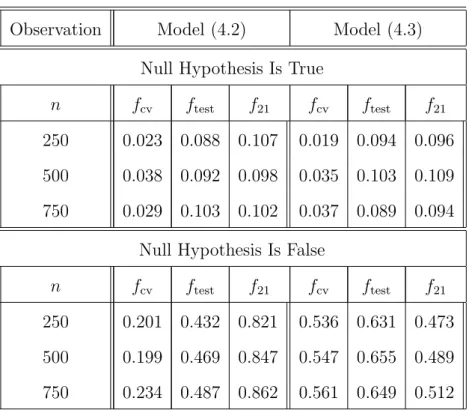
Table 4.2. Sizes and power values for models (4.2) and (4.3) at the α= 10% significance level
Observation Model (4.2) Model (4.3)
Null Hypothesis Is True
n fcv ftest f21 fcv ftest f21
250 0.023 0.088 0.107 0.019 0.094 0.096
500 0.038 0.092 0.098 0.035 0.103 0.109
750 0.029 0.103 0.102 0.037 0.089 0.094
Null Hypothesis Is False
n fcv ftest f21 fcv ftest f21
250 0.201 0.432 0.821 0.536 0.631 0.473
500 0.199 0.469 0.847 0.547 0.655 0.489
Table 4.3. Sizes and power values for models (4.4) and (4.5) at theα = 5% significance level
Observation Model (4.4) Model (4.5)
Null Hypothesis Is True
n fcv ftest f22 fcv ftest f22
250 0.005 0.052 0.049 0.003 0.051 0.048
500 0.004 0.048 0.050 0.007 0.047 0.054
750 0.007 0.051 0.047 0.006 0.052 0.051
Null Hypothesis Is False
n fcv ftest f22 fcv ftest f22
250 0.112 0.164 0.348 0.349 0.423 0.312
500 0.107 0.182 0.387 0.361 0.456 0.331
750 0.132 0.191 0.372 0.358 0.481 0.342
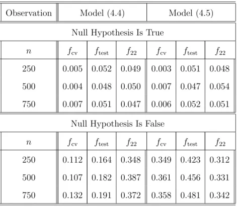
Table 4.4. Sizes and power values for models (4.4) and (4.5) at the α= 10% significance level
Observation Model (4.4) Model (4.5)
Null Hypothesis Is True
n fcv ftest f22 fcv ftest f22
250 0.031 0.110 0.097 0.023 0.089 0.101
500 0.040 0.097 0.102 0.038 0.101 0.097
750 0.033 0.103 0.096 0.033 0.098 0.095
Null Hypothesis Is False
n fcv ftest f22 fcv ftest f22
250 0.197 0.271 0.411 0.452 0.552 0.419
500 0.204 0.267 0.431 0.489 0.581 0.441
Tables 4.1 and 4.2 (columns 2–3 and 5–6) show that the test coupled with a boot-strap critical value (bcv) is more powerful than that associated with the use of an asymptotic critical value (acv) in each case, in addition to the fact that there is serious size distortion when using an acv rather than a bcv. The main reasons are as follows: (a) the rate of convergence of eachLbT(h) to an asymptotic normal distribution is quite slow in this kind of nonparametric setting; and (b) the use of an optimal bandwidth based on the cross–validation selection criterion may not be optimal for testing pur-poses. By contrast, there is only small size distortion between using a bcv and an acv forL21andL22in each implementation, although the version of the test associated with
a bcv has more stable size performance and better power property than that based on
an acv. We therefore compare our nonparametric tests with both L21 and L22 based
on a bcv in each case.
Moreover, Tables 4.1 and 4.2 show that the proposed test is less powerful than the conventional DF test when the true model (4.2) is linear. When the true model (4.3) is nonlinear, however, the DF test is still applicable but is less powerful than the proposed test. Tables 4.3 and 4.4 also show that the proposed test is more powerful than the DK test when the true model (4.5) is nonlinear. When the true model (4.4) is linear, the DK test is more powerful than the proposed test. In summary, Tables 4.1–4.4 show that the proposed test is more powerful in the nonlinear case while the sizes are comparable with the two competitors for the parametric linear case. This supports that the proposed test, which is dedicated to the nonlinear case, is needed to deal with testing stationarity in nonlinear time series models.
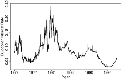
Example 4.2. This example examines the seven–day Eurodollar deposit spot rate
data given in Figure 1 below sampled daily over the period from 1 June 1973 to 25 February 1995, providing 5505 observations.
Let {Yt : t = 1,2,· · · ,5505} be the set of the seven–day Eurodollar deposit spot
rate data. The data set has been studied extensively in the literature. Recent studies (see, for example, Bandi 2002) are concerned with whether {Yt}follows a random walk
model of the form
Yt =µ0+µ1t+Yt−1+ut, (4.10)
where {ut} is a sequence of strictly stationary errors.
We consider a special form of (1.3) with Xτ
1973 1977 1981 1985 1990 1994 0.05 0.10 0.15 0.20 0.25 Year
Eurodollar Interest Rate
Figure 1: Plot of the seven–day Eurodollar deposit spot rate data order to apply model (1.3) to test whether {Yt}follows (4.10), it suffices to test
H0 : vt=vt−1+ut for Yt=β0+β1t+β2t2+vt. (4.11)
To apply the testLbT(bhtest) to determine whether{Yt}follows a random walk model of the form Yt=µ0+µ1t+Yt−1+ut, we need to propose the following procedure for
computing the p–value of LbT(bhtest):
• For the real data set, compute bhtest and LbT(bhtest).
• Let Y1∗ = Y1. Generate Yt∗ = Yt∗−1 + (Xt−Xt−1) τ b β +u∗t for 2 ≤ t ≤ 5505, where u∗t = butηt, in which but = Yt −Yt−1 −(Xt−Xt−1) τ b β and {ηt} is chosen
as a sequence of independent random variables with the following distributional
structure: P η1 =− √ 5−1 2 = √ 5+1 2√5 and P η1 = √ 5+1 2 = √ 5−1 2√5 . Such two–
point distributional structure has been commonly used in the literature (see, for example, Li and Wang 1998).
• Compute the corresponding version Lb∗T(bhtest) based on {Yt∗}.
• Repeat the above steps N times to find the bootstrap distribution of Lb∗T(bhtest) and then compute the proportion that LbT(bhtest) <Lb∗T(bhtest). This proportion is an approximate p–value of LbT(bhtest).
Our simulation results return the simulated p–values of pb1 = 0.007 for L22 and
b
no enough evidence of accepting the unit–root structure at the 5% significance level, there is some evidence of accepting the unit–root structure based on LbT(bhtest) at the 1% significance level. This supports the existing conclusions made in Bandi (2002).
5. Conclusion. We have proposed a new nonparametric test for the parametric
specification of the residuals. An asymptotically normal distribution of the proposed test has been established. In addition, we have also proposed the Simulation Scheme to implement the proposed test in practice. The small and medium–sample results show that both the proposed test and the Simulation Scheme are practically applicable and implementable.
This paper has focused on the case where{Xt}is a vector of deterministic regressors.
The case where{Xt}is a vector of stochastic regressors is equally important. Discussion
of such a case requires developing new theory and also involves more technicalities. It is therefore left for future research.
6. Acknowledgments. The authors would like to thank Dr Jiying Yin for his
excellent computing assistance and the Australian Research Council Discovery Grants under Grant Numbers: DP0558602 and DP0879088 for the financial support.
Appendix A
In this appendix, we introduce several technical conditions and then give some lemmas for the proofs of Theorems 2.1 and 3.1. Assumptions A.1–A.3 are imposed for Case A and Assumptions A.1–A.5 are needed for Case B. To avoid adding some non–essential technicalities, we assume the following initial values Y0∗ = y0∗ = 0 and
X0 =x0 = 0, v0 = 0 and v0∗ = 0 throughout this appendix. A.1. Assumptions
Assumption A.1. (i)Let K(·) be a symmetric probability density function with compact
supportC(K). Let also the existence ofK(3)(·), the three–time convolution ofK(·)with itself. In addition, there is some positive function M(·) such that
|K(x+y)−K(x)| ≤M(x) |y|
for all x∈C(K) and any smally, where M(·)≥0 is assumed to satisfy R
M2(u)du <∞. (ii) For Case A, let h satisfy limT→∞T
3
10h = 0 and lim sup
T→∞T 1
2−0h = ∞ for any 0< 0 < 15. Let h satisfy limT→∞h= 0 and lim supT→∞T h=∞ for Case B.
Assumption A.2. For i= 1,2, let lim T→∞ hPT t=2 Pt−1 s=1 ||Zt||i||Zs||i √ t−s R2Ti λiT = 0, (A.1) lim T→∞ PT t=2 Pt−1 s=1||Zt||i ||Zt−√1−Zs−1||i t−s ||Zs|| i R3i T λiT = 0, (A.2)
where Zt=Xt−Xt−1 for Case A and Zt=Xt for Case B, λT =T
3 4
√
h, RT is chosen such
that Assumption A.3 below holds, and || · || denotes the Euclidean norm.
Assumption A.3. (i) Let H0 be true. Then there are some βband RT → ∞ such that
lim T→∞P RT||βb−β||> B0 < ε0
for any ε0 >0 and some B0 >0.
(ii)LetH0 be true. There is an estimatorβb∗ such that for some positive constantsB0∗ >0
and ε∗0 the following inequality
lim T→∞P RT||βb∗−βb||> B0∗|WT < ε∗0
holds with probability one with respect to the distribution of WT, where RT → ∞ is the same
as in (i).
Assumption A.4. (i) Let H0 be true. Then there is an estimatorθb0 such that lim T→∞P √ T||θb0−θ0||> C0 < 0
for any 0 >0 and some C0>0
(ii) Let π0(v) denote the marginal density of {vt} under H0 for Case B. Suppose that π0(v) is continuous and that f0(v, θ) is differentiable in both v and θ. In addition,
0< Z ∂f0(v, θ0) ∂v 2 π02(v)dv <∞ and 0< Z ∂f0(v, θ0) ∂θ 2 π20(v) dv <∞.
Assumption A.5. (i) Let H0 be true. Then there is an estimatorθb∗0 such that for some
positive constants C0∗ >0 and ∗0 the following inequality
lim T→∞P √ T||θb∗0−θ0b||> C0∗|WT < ∗0
holds with probability one with respect to the distribution of WT.
(ii)Let H1 be true. There exists an estimatorθb1 such that lim T→∞P √ T||θb1−θ1||> C1 < 1
(iii) Let π1(v) denote the marginal density of {vt} under H1 for either A or Case B.
Suppose thatπ1(v)is continuous and thatf1(v, θ)is differentiable in bothvandθ. In addition,
0< Z ∂f1(v, θ1) ∂v 2 π12(v)dv <∞ and 0< Z ∂f1(v, θ1) ∂θ 2 π21(v) dv <∞.
Assumption A.1(i) is a mild condition and holds in many cases. For example, Assumption A.1(i) holds when K(x) = 12I[−1,1](x). While Assumption A.1(ii) imposes certain conditions, which may look more restrictive than those for the stationary case, they don’t look unnatural in the nonstationary case. The corresponding conditions on the bandwidth for nonparametric testing in the stationary case are the same as the minimal conditions: limT→∞h = 0 and limT→∞T h=∞ that are assumed for nonparametric kernel testing for the case where both the regressors and errors are independent (see, for example, Gao 2007).
Assumption A.2 imposes some minimal conditions on the trend function such that poly-nomial trends are included. Consider the case where Xt =t2 for Case A, we have for some
0< C1, C2 <∞ T X t=2 t−1 X s=1 |Zt| 1 √ t−s|Zs| ≤C1 T X t=2 t−1 X s=1 st √ t−s =O T72 , RT2 = T X t=1 Zt2 =C2 T3 and T32 b β−β →N(0, σ21), whereZt=Xt−Xt−1,βb= PT t=1Zt(Yt−Yt−1) PT t=1Zt2
is the ordinary least squares estimator ofβbased on a model of the form Yt−Yt−1= (Xt−Xt−1)β+ut, and σ1 is a positive constant.
In this case, equations (A.1) and (A.2) become respectively hPT t=2 Pt−1 s=1 |Zt√|·|Zs| t−s R2T λT = O T 7 2h T3+34 √ h ! =O √ h T14 ! =o(1), PT t=2 Pt−1 s=1|Zt| |Zt−√1−Zs−1| t−s |Zs| RT3 λT = O T 9 2 T92+ 3 4 √ h ! =O 1 T34 √ h =o(1).
Similarly, in the case whereXt=t2 for Case B, we have for some 0< D1, D2 <∞
T X t=2 t−1 X s=1 |Xt| 1 √ t−s|Xs| ≤D1 T X t=2 t−1 X s=1 s2t2 √ t−s =O T112 , RT2 = T X t=1 Xt2 =D2 T5 andT52 b β−β →N(0, σ22), (A.3) where βb = PT t=1XtYt PT t=1Xt2
is the ordinary least squares estimator of β based on a model of the form Yt=Xtβ+vt, and σ2 is a positive constant.
In this case, equations (A.1) and (A.2) become respectively hPT t=2 Pt−1 s=1 |Xt√|·|Xs| t−s R2T λT = O T 11 2 h T5+34 √ h ! =O √ h T14 ! =o(1), PT t=2 Pt−1 s=1|Xt| |Xt−√1−Xs−1| t−s |Xs| R3 T λT = O T 15 2 T152+ 3 4 √ h ! =O 1 T34 √ h =o(1).
Thus, equations (A.1) and (A.2) hold for i = 1. Similarly, we can show that the other cases for (A.1) and (A.2) all hold. In addition, Assumption A.2 is satisfied automatically when the trend functions are all continuous and bounded.
Assumption A.3 requires that the conventional rate of convergence for the parametric case is achievable even when {vt} is nonstationary. WhenXt=t2, it has been shown above
that the rate of convergence ofβbtoβ is proportional toT
3
2 in Case A and T 5
2 in Case B. Assumption A.4 imposes the differentiability conditions as well as the moment conditions onf0(·,·). As{vt}is strictly stationary, it is possible to verify Assumption A.4 in many cases.
Assumption A.5(i) is the bootstrap version of Assumption A.4(i). Assumption A.5(ii)(iii) is a kind of corresponding version of Assumption A.4 underH1. Note that Assumptions A.4(i) and A.5(i)(ii) may also be satisfied even when{ut}is correlated. In this case, an instrumental–
variable method may be used to construct a consistent estimator (see, for example, Fr¨olich 2008)
A.2. Proof of Theorem 2.1 in Case A
Letσu2 =E[u21]≡1 throughout the rest of this paper. To avoid notational complication, we introduce ast =Kh t−1 X i=s ui ! and ηt= 2 t−1 X s=1 ast us. Observe that c MT ≡ T X t=1 T X s=1,6=t b us Kh(bvs−1−bvt−1) ubt= T X t=1 T X s=1,6=t us Kh(vs−1−vt−1) ut + T X t=1 T X s=1,6=t e us Kh(bvs−1−bvt−1) uet+ 2 T X t=1 T X s=1,6=t us Kh(bvs−1−bvt−1) eut + MT4 ≡MT1+MT2+MT3+MT4, (A.4) b σ2T ≡ 2 T X t=1 T X s=1,6=t b u2s Kh2(bvs−1−vbt−1) bu 2 t = 2 T X t=1 T X s=1,s6=t u2s Kh2(vs−1−vt−1) u2t + 2 T X t=1 T X s=1,6=t e u2s Kh2(bvs−1−vbt−1) eu 2 t + 2 T X t=1 T X s=1,6=t u2s Kh2(bvs−1−bvt−1) eu 2 t + σeT24≡eσ2T1+σeT22+eσT23+σe2T4, (A.5)
where for Case A under H0: vt=vt−1+ut, b ut = bvt−vbt−1=Yt−X τ tβb− Yt−1−Xtτ−1βb = (Xt−Xt−1)τ β−βb +vt−vt−1 = ut+ (Xt−Xt−1)τ β−βb ≡ut+uet, e ut = (Xt−Xt−1)τ β−βb , b vs−1−bvt−1 = vs−1−vt−1+ (Xs−1−Xt−1) τ (β−βb), MT4 = McT −MT1−MT2−MT3, e σT24 = bσT2 −σe2T1−eσT22−σe2T3.
In view of (A.4) and (A.5), in order to prove Theorem 2.1 for Case A, it suffices to show that as T → ∞ MT1 e σT1 →D N(0,1), (A.6) MT i e σT1 →P 0 fori= 2,3,4, (A.7) e σT j e σT1 →P 0 forj = 2,3,4. (A.8)
We will return to the proof of (A.7) and (A.8) in Lemma A.5 after having proved (A.6) in Lemmas A.1–A.4 below. In order to prove (A.6), we need to apply Lemma B.1 of Appendix B below.
Before verifying the conditions of the Lemma B.1, we introduce the following notation. Let YT t = ηtutσT 1, ΩT ,s = σ{YT t : 1 ≤ t ≤ s} be a σ–field generated by {YT t : 1 ≤ t ≤ s}, GT = ΩT ,M(T) and GT ,s be defined by GT ,s= ΩT ,M(T), 1≤s≤M(T), ΩT ,s, M(T) + 1≤s≤T , (A.9) where σ2T,1 = varhPT t=2ηtut i
and M(T) is chosen such that M(T) → ∞ and MT(T) → 0 as T → ∞. LetUeM2 (T)= e σ2 M(T),1 σ2 M(T),1 , whereσS,21= varhPS t=2ηtut i
for all 1≤S≤T. We can show that as T → ∞ e σ2T1 σ2 T1 −UeM2 (T)→P 0. (A.10)
Thus, condition (B.2) of the Lemma B.1 of Appendix B below can be satisfied. The proof of (A.10) is given in Lemma A.4 below.
Therefore, in view of the Lemma B.1, in order to prove that asT → ∞
MT1 e σT1 = 1 e σT1 T X t=2 ηtut→D N(0,1), (A.11)
it suffices to show that there is an almost surely finite random variable ξ such that for all >0, T X t=2 E YT t2I{[YT t|>]}(YT t)|ΩT ,t−1 →P 0, (A.12) T X t=2 E[YT t|GT ,t−1] = M(T) X t=2 YT t+ T X t=M(T)+1 E[YT t|ΩT ,t−1] = M(T) X t=2 YT t→P 0, (A.13) T X t=2 |E[YT t|GT ,t−1]| 2 = M(T) X t=2 YT t2 + T X t=M(T)+1 |E[YT t|ΩT ,t−1]| 2 = M(T) X t=2 YT t2 →P 0, (A.14) lim δ→0lim infT→∞P e σT1 σT1 > = 1, (A.15)
where IA(x) is the conventional indicator of the form IA(x) = 1 when x ∈A and IA(x) = 0
when x 6∈ A. The proof of (A.12) follows from Lemma A.2 below. The proof of (A.13) is similar to that of (A.14), which follows from
M(T) X t=2 EYT t2=O M(T) T 3 2 ! →0 (A.16)
asT → ∞, in which Lemma A.1 below is used. In order to prove (A.12), it suffices to show that
1 σT41 T X t=2 E ηt4 →0, (A.17)
which is given in Lemma A.2 below. The proof of (A.15) follows from
e
σT21 σ2
T1
→D ξ2 >0, (A.18)
which is given in Lemma A.3 below.
Before we establish several lemmas for the proof of Theorem 2.1, we need to introduce the following notation.
For anyt > s≥1 and α= 12, definevst = vtCα−1(−t−vss)−α1, where 0< Cα<∞ is a normalized
constant. We assume without loss of generality thatCα= 1 in this appendix. Recall thatg(u)
is the marginal density of the stationary time series {ut}. Let fst(·) be the density function
of vst and gst(·) be the density function of ust = vt−1 −vs−1. Then, the i–th derivative of gst(v) satisfies fori= 0,1 g(sti)(v) = 1 Cα(t−s)(1+i)α fst(i) v (t−s)α . (A.19)
Similarly, letf(·|Fs) andg(·|Fs) be the conditional density functions ofvst andust given
Fs−1, where{Fs}is a sequence of σ–fields such that{vs} is adapted toFs. Then
gst(v|Fs−1) = 1 Cα(t−s)α fst v (t−s)α|Fs−1 , (A.20)
and the first derivatives of gst(·|Fs−1) and fst(·|Fs−1) satisfy g(1)st (v|Fs−1) = 1 Cα(t−s)2α fst(1) v (t−s)α|Fs−1 . (A.21)
Assumption 2.1(ii) then implies the following useful results: ast−s→ ∞
sup |x|≤δ f (i) st (x) =O(1), (A.22) sup |x|≤δ f (i) st (x|Fs−1) =OP(1) (A.23)
for i = 0,1, where δ > 0 is some small constant. Equations (A.22) and (A.23) are used repeatedly in the proofs of Lemmas A.1–A.5 below.
Lemma A.1. Let Assumptions 2.1 and A.1 hold. Then for large enoughT
σ2T1= var " T X t=2 ηtut # = 16 R K2(x)dx 3√2π T 3/2h (1 +o(1)). (A.24)
Proof: It follows from the definition that
σT21 = E " T X t=1 ηtut #2 = 2 T X t=1 T X s=1 Ea2stu2su2t+ 4 T X t=2 t−1 X s16=s2=1 Eas1tas2tus1us2u 2 t = 2σ2u T X t=1 T X s=1 E a2stu2s +R1T, (A.25) where R1T = 4σ2u PT t=2 Pt−1 s16=s2=1E[as1tas2tus1us2].
Letwst =Pti−=1s+1ui andgst(·,·) be the joint density function ofwst and us. Assumption
2.1(ii) then implies E[a2stu2s] = Z Z Kh2(wst+us)us2gst(ust, us)dusdust = Z Z Kh2(ust+us)u2sgst(wst|us)f(us)dusdust = 1 (t−s−1)α Z Z Kh2(wst+us)u2sfst ust (t−s−1)α|us g(us)dusdust = h (t−s−1)α Z Z K2(xst)x2fst xsth (t−s−1)α|us g(x)dxdxst. (A.26)
Choose mT ≥1 such thatmT → ∞ and √mTT h →0 as T → ∞. Observe that
T X t=2 t−1 X s=1 E[a2stu2s] = T−1 X s=1 T X t=s+1 E[a2stu2s] =A1T +A2T, (A.27) whereA1T =PTs=1−1 P 1≤(t−s)≤mTE[a 2
stu2s] =O(T mT) =o(T3/2h) using the fact thatE
a2stu2s≤
k20E
u2s
Using Assumption 2.1, it follows from (A.26) that A2T = T−1 X s=1 X mT+1≤(t−s)≤T−1 E[a2stu2s] = (1 +o(1))C0 T−1 X s=1 X mT+1≤(t−s)≤T−1 h (t−s−1)α Z Z K2(y)x2g(x)dxdy = 4σ 2 u R K2(y)dy 3 C0T 3/2h(1 +o(1)). (A.28)
To deal with R1T, we need to introduce the following notation: for 1≤i≤2,
Zi=usi, Z11= t−1 X i=s1+1 ui, Z22= s1−1 X j=s2+1 uj, (A.29)
ignoring the notational involvement of s,tand others.
Letg(x11, x1, x22, x2) be the joint density of (Z11, Z1, Z22, Z2),g11(x11|x1, x22, x2) be the conditional density function ofZ11given (Z1, Z22, Z2),g(x1|x22, x2) be the conditional density function ofZ1 given (Z22, Z2), andg22(x22|x2) be the conditional density function ofZ22given Z2. Similarly to (A.26), we have that for large enoughT
E[as1tas2tus1us2] =E Kh t−1 X i=s1 ui ! Kh t−1 X j=s2 uj us1us2 = E[Z1Z2Kh(Z2+Z22)Kh(Z1+Z2+Z11+Z22)] = Z · · · Z x1x2Kh(x1+x2+x11+x22)Kh(x2+x22) ×g(x11, x1, x22, x2)dx1dx2dx11dx22 = Z · · · Z x1x2Kh(x1+x2+x11+x22)Kh(x2+x22) ×g11(x11|x1, x22, x2)g(x1|x22, x2)g22(x22|x2)g(x2)dx1dx2dx11dx22 (usingyii= xi+hxii) =h2 Z · · · Z K(y22)K(y11+y22)x1x2 ×g11(y11h−x1|x1, y22h, x2)g(x1|hy22, x2)g22(hy22−x2|x2)g(x2) ×dx1dx2dy11dy22
(using Taylor expansions) = h2(1 +o(1))
Z · · ·
Z
K(y22)K(y11+y22)x1x2
×g11(−x1|x1,0, x2)g(x1|0, x2)g22(−x2|x2)g(x2)dx1dx2dy11dy22 +h4(1 +o(1)) Z · · · Z K(y22)K(y11+y22)x1x2 ×g011(−x1|x1,0, x2)g(x1|0, x2)g220 (−x2|x2)g(x2)dx1dx2dy11dy22
= h2(1 +o(1)) Z · · · Z K(y22)K(y11+y22)x1x2g(x1|0, x2)g(x2) × 1 (t−s1−1)α 1 (s1−s2−1)α f11 − x1 (t−s1−1)α |x1,0, x2 ×f22 − x2 (s1−s2−1)α|x2 dx1dx2dy11dy22 +h4(1 +o(1)) Z · · · Z y11y22K(y22)K(y11+y22)x1x2g(x1|0, x2)g(x2) × 1 (t−s1−1)2α 1 (s1−s2−1)2α f110 − x1 (t−s1−1)α |x1,0, x2 ×f220 − x2 (s1−s2−1)α |x2 dx1dx2dy11dy22. (A.30) Thus, similarly to (A.27) and (A.28), we can show
T X t=2 t−1 X s16=s2=1 E[as1tas2tus1us2] = 2 T X t=3 t−1 X s1=2 s1−1 X s2=1 E[as1tas2tus1us2] = o T3/2h + 2C02h2(1 +o(1)) T X t=3 t−1 X s1=2 s1−1 X s2=1 1 (t−s1−1)α 1 (s1−s2−1)α × Z · · · Z K(y22)K(y11+y22)x1x2g(x1|0, x2)g(x2)dx1dx2dy11dy22 +o T3/2h + 2h4(1 +o(1)) T X t=3 t−1 X s1=2 s1−1 X s2=1 1 (t−s1−1)2α 1 (s1−s2−1)2α × Z · · · Z
y11y22K(y22)K(y11+y22)x1x2g(x1|0, x2)g(x2)dx1dx2dy11dy22 = o T3/2h (A.31) using Assumption 2.1.
Equations (A.27), (A.28) and (A.31) show that for large enoughT σT21 = 16
R
K2(y)dy 3√2π T
3/2h(1 +o(1)). (A.32)
The proof of Lemma A.1 is therefore finished.
Lemma A.2. Let Assumptions 2.1 and A.1 hold. Then for large enoughT
lim T→∞ 1 σ4 T1 T X t=2 Eηt4= 0. (A.33)
Proof. Observe that Eη4t= 16 t−1 X s1=1 t−1 X s2=1 t−1 X s3=1 t−1 X s4=1 E[as1tas2tas3tas4tus1us2us3us4]. (A.34)
We mainly consider the cases ofsi 6=sj for alli6=jin the following proof. Since the other
loss of generality, we only look at the case of 1≤s4 < s3 < s2 < s1 ≤t−1 in the following evaluation. Let us1t = us1 + t−1 X i=s1+1 ui, us2t=us1+us2 + s1−1 X i=s2+1 ui+ t−1 X j=s1+1 uj, us3t = us1 +us2 +us3 + s2−1 X k=s3+1 uk+ s1−1 X i=s2+1 ui+ t−1 X j=s1+1 uj, us4t = us1 +us2 +us3 +us4+ s3−1 X l=s4+1 ul+ s2−1 X k=s3+1 uk+ s1−1 X i=s2+1 ui+ t−1 X j=s1+1 uj.
Similarly to (A.29), let againZi=usi for 1≤i≤4,
Z11= t−1 X i=s1+1 ui, Z22= s1−1 X j=s2+1 uj, Z33= s2−1 X k=s3+1 uk, Z44= s3−1 X l=s4+1 ul.
Analogously to (A.30), we may have E " 4 Y i=1 asitusi # =E 4 Y j=1 ZjKh j X i=1 [Zi+Zii] ! = Z · · · Z g(x11, x1,· · · , x44, x4) × 4 Y j=1 Kh j X i=1 [xi+xii] ! xjdxjjdxj ! = Z · · · Z g11(x11|x1,· · · , x44, x4)g(x1|x22,· · · , x44, x4) ×g22(x22|x2,· · ·, x44, x4)g(x2|x33,· · · , x44, x4) ×g33(x33|x3, x44, x4)g(x3|x44, x4)g44(x44|x4)g(x4) × 4 Y j=1 Kh j X i=1 [xi+xii] ! xjdxjjdxj !
(using yii= xi+hxii andyi =xi)
=h4
Z · · ·
Z
g11(y11h−y1|y1,· · ·, hy44, y4)g(y1|hy22,· · ·, hy44, y4)
×g22(hy22−y2|y2,· · ·, hy44, y4)g(y2|hy33,· · ·, hy44, y4)
×g33(hy33−y3|y3, hy44, y4)g(y3|hy44, y4)g44(hy44−y4|y4)g(y4)
× 4 Y j=1 K j X i=1 yii ! yjdyjjdyj ! =h4(1 +o(1)) Z · · · Z g11(−y1|y1,· · · ,0, y4)g(y1|0,· · ·,0, y4) ×g22(−y2|y2,· · ·,0, y4)g(y2|0,· · · ,0, y4) ×g33(−y3|y3,0, y4)g(y3|0, y4)g44(−y4|y4)g(y4) × 4 Y j=1 K j X i=1 yii ! yjdyjjdyj ! , (A.35)
where C22(K)≡Q4 j=1 R yjjK Pj i=1yii dyjj <∞ involved in (A.35).
Hence, similarly to (A.31) we have by Assumption 2.1
T X t=2 X 1≤s4<s3<s2<s1≤t−1 E[as1tas2tas3tas4tus1us2us3us4] =O h4 T X t=2 X 1≤s4<s3<s2<s1≤t−1 1 √ t−s1 1 √ s1−s2 1 √ s2−s3 1 √ s3−s4 =O T3h4=o T3h2. (A.36)
Analogously, we can deal with the other terms of (A.34) as follows:
T X t=2 X 1≤s26=s1≤t−1 Ea2s1ta2s2tus21u2s2 = o T3h2, (A.37) T X t=2 X 1≤s36=s26=s1≤t−1 Ea2s1tas2tas3tu 2 s1us2us3 = o T3h2, (A.38) T X t=2 X 1≤s26=s1≤t−1 E a3s1tas2tu 3 s1us2 = o T3h2 . (A.39)
Thus, the proof of (A.33) is completed using (A.34)–(A.39).
Lemma A.3. Let Assumptions 2.1 and A.1 hold. Then as T → ∞ e σT21 σT21 →D ξ 2 >0 (A.40) with ξ2 = √ π
2 M12(1), where M12(·) is a special case of the Mittag–Leffer process Mβ(·) with β = 12 as described by Karlsen and Tjøstheim (2001, p.388).
Proof. To simplify the following proof, ignoring the higher–order term we rewrite σT21 = 16σ 4 uJ02 3√2π T 3/2h≡C10T3/2h. (A.41) Let Q(u) = KJ2(u)
02 and N(T) be the same as T(n) in Karlsen and Tjøstheim (2001). It then follows from Lemma B.2 below that as T → ∞
max 1≤t≤T 1 N(T)h T X s=2 Q vs−1−vt−1 h −1
=o(1) almost surely. (A.42)
Meanwhile, Theorem 3.2 of Karlsen and Tjøstheim (2001, p.389) is applicable to the current case of vt=vt−1+ut under H0 to show that asT → ∞
N(T)
L0√T →D M12(1) (A.43) when the slowly–varying function in this case is L0= 2
√ 2 3 .
Therefore, equations (A.42) and (A.43) imply asT → ∞ 4 σT21 T X t=1 T X s=1 a2st ! u2t = 2 T C10 T X t=1 u2t √1 T h T X s=1 a2st ! = 2L0J02 C10 N(T) L0 √ T 1 T T X t=1 u2t 1 N(T)h T X s=1 Q vs−1−vt−1 h −1 ! +2L0J02 C10 N(T) L0 √ T 1 T T X t=1 u2t →D 2 J02L0 C10 M1 2(1) = √ π 2 M12(1) ≡ξ2. (A.44) Therefore, equation (A.44) completes the proof of Lemma A.3.
Lemma A.4. Let Assumptions 2.1 and A.1 hold. Then as T → ∞, M(T) → ∞ and
M(T) T →0 e σT21 σT21 − e σM2 (T),1 σM2 (T),1 →P 0. (A.45) Proof. To simplify our proofs, we introduce the following lower case notation: m =T, n=M(T),σ2m=σ2T1,σn2 =σM2 (T),1, and for 1≤i≤n, 1≤j≤i−1, eij = u2i −E[u2i] Kh2 i−1 X l=j ul u2j and Wmi= 1 σ2 m i−1 X j=1 eij. (A.46) wi2 = i−1 X j=1 Kh2 i−1 X l=j ul u2j = i−1 X j=1 Kh2 i−1 X l=j+1 ul+uj u2j. (A.47) Note thatWmi= σ12 m u 2 i −E[u21] w2i. Observe that e σ2m1 σ2m1 − e σ2n1 σ2n1 = m X i=1 Wmi− n X j=1 Wnj+E[u21] 1 σ2 m m X i=1 w2i − 1 σ2 n n X j=1 w2j ≡ Imn+E[u21]Jmn. (A.48)
In view of (A.47), in order to prove (A.45), it suffices to show that asm, n→ ∞
Imn→P 0 and Jmn→P 0. (A.49)
We start by proving the second part of (A.49). Observe also that
E Jmn2 = E 1 σ2 m m X i=1 w2i − 1 σ2 n n X j=1 wj2 2 =E 1 σ2 m m X i=n+1 w2i +σ 2 n−σm2 σ2 m σn2 n X j=1 w2j 2 = 1 σ4 m m X i=n+1 m X k=n+1 Ew2kw2i+ σ 2 n−σ2m 2 σ4 m σ4n n X j=1 n X k=1 Ew2kwj2 − 2σ 2 m−σn2 σ4 m σ2n m X i=n+1 n X j=1 Ew2iwj2. (A.50)
We first deal with the first term. Recallingaji=Kh Pi−1 l=jul , we have E m X i=n+1 w2i !2 =E m X i=n+1 m X j=n+1 w2i wj2 = m X i=n+1 E[w4i] + m X i=n+1 m X j=n+1,6=i E[wi2 w2j]. (A.51)
We now evaluate the orders of Pm
i=n+1E[w4i] and
Pm
i=n+1
Pm
j=n+1,6=iE[w2i w2j]
respec-tively. To do so, we now consider one of the cases: 1≤t≤s−1; 2≤s≤j−1;n+ 1≤j ≤
i−1;n+ 2≤i≤m for the following term
E m X i=n+2 i−1 X j=n+1 j−1 X s=2 s−1 X t=1 a2siu2sa2tju2t = m X i=n+2 i−1 X j=n+1 j−1 X s=2 s−1 X t=1 E a2siu2sa2tju2t = m X i=n+2 i−1 X j=n+1 j−1 X s=2 s−1 X t=1 E Kh2 j−1 X c=s+1 uc+ i−1 X c=j uc+us u2s × Kh2 s−1 X d=t+1 ud+ j−1 X d=s+1 ud+us+ut ! u2t # .
Other terms may be dealt with similarly. To simplify our calculation, we now introduce the following simplistic symbols: Z11=Ps−1
d=t+1ud,Z22= Pj−1 c=s+1uc,Z33= Pi−1 c=juc,Z1=ut and Z2 =us.
As in the proof of Lemma A.1, using the same techniques as in (A.35) we have
E " Kh2 2 X i=1 (Zi+Zii) ! Kh2(Z2+Z22+Z33)Z12Z22 # = Z · · · Z Kh2 2 X i=1 (xi+xii) ! Kh2(x2+x22+x33) x21 x22 ×g(x33, x22, x2, x11, x1) dx33dx22dx11dx1dx2 = Z · · · Z Kh2 2 X i=1 (xi+xii) ! Kh2(x2+x22+x33) x21 x22 ×g33(x33|x22, x2, x11, x1)g22(x22|x2, x11, x1)g(x2|x11, x1)g11(x11|x1)g(x1) ×dx33dx22dx11dx1dx2
(usingyi =xi and yii= xi+hxii fori= 1,2 andy33= xh33)
=h3
Z · · ·
Z
K2(y11+y22)K2(y22+y33) y21y22
×g33(y33h|y22h−y2, y2, y11h−y1, y1)g22(y22h−y2|y2, y11h−y1, y1)
×g11(y11h−y1|y1)g(y2|y11h−y1, y1)g(y1) dy33dy22dy11dy1dy2 =h3(1 +o(1))
Z · · ·
Z
K2(y11+y22)K2(y22+y33) y21y22
×g33(0| −y2, y2,−y1, y1)g22(−y2|y2,−y1, y1)g11(−y1|y1)
=h3(1 +o(1)) Z · · · Z K2(y11+y22)K2(y22+y33)y12y22 ×f33(0| −y2, y2,−y1, y1)f22 − y2 (j−s−1)α|y2,−y1, y1 ×f11 − y1 (s−t−1)α|y1 g(y2| −y1, y1)g(y1) dy33dy22dy11dy1dy2. (A.52) In view of (A.52) and (A.52), similarly to the calculations of (A.26), (A.27) and (A.28), it can be shown that for large enough mand n,
E m X i=n+1 m X j=n+1,6=i w2i w2j = m X i=n+1 m X j=n+1,6=i Ewi2 w2j = Ch3(1 +o(1)) m X i=n+2 i−1 X j=n+1 j−1 X s=2 s−1 X t=1 1 (i−j)α 1 (j−s−1)α 1 (s−t−1)α = Ch3(1 +o(1))(m−n)52. (A.53) Similarly to (A.53), we may have for sufficiently largem and n,
m X i=n+1 E[w4i] = Ch2(1 +o(1))(m−n)32. (A.54) E m X i=n+1 n X j=1 w2i wj2 = o h3(m−n)52 , (A.55) E m X i= n X j=1 w2i wj2 = o h3(m−n)52 (A.56) using limm,n→∞ mn = 0.
Thus, equations (A.50)–(A.56) imply that for large enoughm and n,
EJmn2 = E 1 σ2 m m X i=1 wi2− 1 σ2 n n X j=1 w2j 2 = 1 σ4 m m X i=n+1 m X k=n+1 Ew2kwi2+ σ 2 n−σm2 2 σ4 m σn4 n X j=1 n X k=1 Ewk2w2j − 2σ 2 m−σn2 σ4 m σn2 m X i=n+1 n X j=1 Ewi2w2j = Ch1− n m 32 (1 +o(1)) =o(1) (A.57) using again limm,n→∞ mn = 0. We thus complete the second part of (A.49).
Letzi =u2i −E[u21]. We now come back to prove the first part of (A.49). Note that for n+ 1≤i≤mand 1≤j≤n, Imn= 1 σ2 m m X i=1 u2i −E[u21]w2i − 1 σ2 n n X j=1 u2j−E[u21]wj2= 1 σ2 m m X i=1 zi w2i − 1 σ2 n n X j=1 zj w2j. (A.58)
Note that{w2
i} is a function of{uj : 1≤j≤i−1} while {zi}is a function of {ui}. Let
gzw(·,·) be the joint density function of (zi, wi2),gz|w(·|·) be the conditional density function
of zi given wi, and gw(·) be the marginal density function of wi2. Obviously, gzw(z, w) =
gz(z)gw(w) when{ui} is assumed to be a sequence of independent random variables.
Thus, in view of the relationshipgzw(z, w) =gz|w(z|w)gw(w) and the fact that the
condi-tional moments ofzigivenwido not affect the order ofE
Imn2 , by using the same arguments as in (A.50)–(A.57), we can show that for large enough m and n,
E Imn2 = E 1 σ2 m m X i=1 zi wi2− 1 σ2 n n X j=1 zj w2j 2 = 1 σ4 m m X i=n+1 m X k=n+1 Ezk w2k zi w2i + σ 2 n−σm2 2 σ4 m σn4 n X j=1 n X k=1 Ezk wk2 zj w2j − 2σ 2 m−σn2 σ4 m σn2 m X i=n+1 n X j=1 Ezi wi2 zj w2j = Ch 1− n m 3 2 (1 +o(1)) =o(1). (A.59) We therefore have completed the proof of Lemma A.4.
Lemma A.5. Let the conditions of Theorem 2.1 hold. Then as T → ∞
MT i e σT1 →P 0 fori= 2,3,4, (A.60) e σT j e σT1 →P 0 forj= 2,3,4. (A.61) Proof: Since eσ 2 T1 σ2 T1
→D ξ2 as shown in Lemma A.3, in order to prove (A.60) and (A.61),
it suffices to show that asT → ∞
MT i σT1 →P 0 fori= 2,3,4, (A.62) e σT j σT1 →P 0 forj= 2,3,4. (A.63)
Since the details are very similar, we prove only (A.62) fori= 2. Observe that
MT2 = T X t=1 T X s=1,6=t e us Kh(bvs−1−bvt−1) eut= T X t=1 T X s=1,6=t e us Kh(vs−1−vt−1) uet + T X t=1 T X s=1,6=t e us (Kh(bvs−1−vbt−1)−Kh(vs−1−vt−1)) eut ≡ MT21+MT22. (A.64)
For someB0>0, let Θ(β) = n
b
β : ||βb−β|| ≤B0R−T1 o
and IΘ(β)(βb) be the conventional indicator function. Thus, for sufficiently large T and any given >0,
P MT21IΘ(β)(βb) ≥σT1 ≤ E MT21IΘ(β)(βb) σT1 ≤ PT t=1 PT s=1,6=tE h |ues| Kh(vs−1−vt−1) |eut|IΘ(β)(βb) i σT1 ≤C PT t=1 PT s=1,6=t||Xs−Xs−1|| E[Kh(vs−1−vt−1)] ||Xt−Xt−1|| R2TσT1 ≤C 2hPT s=2 Ps−1 t=1||Xs−Xs−1|| √s1−t ||Xt−Xt−1|| RT2σT1 =o(1) (A.65) using uet= (Xt−Xt−1) τβ− b β
, recalling the definition of Kh(·) =K h·
, the first part of Assumption A.2 and for all s > t,E[Kh(vs−1−vt−1)]≤ √Chs−t, which follows from
E[Kh(vs−1−vt−1)] = E K vs−1−vt−1 h = √h s−t Z K(x)fst xh √ s−t dx ≤ C√h s−t,
using the same argument as in (A.26) of the proof of Lemma A.1, wherefst(·) is the density
of vst = vs−√1−s−vtt−1 and fst xh √ s−t
is bounded by (2.6) of Assumption 2.1(i). Therefore, for sufficiently small >0
P(|MT21| ≥σT1) = P (|MT21| ≥σT1)∩ b β6∈Θ(β) + P(|MT21| ≥σT1)∩ b β∈Θ(β) ≤ P ||βb−β||> B0RT−1 +P MT21IΘ(β)(βb) ≥σT1 → 0 as T → ∞. (A.66) In view ofbvs−1−bvt−1 =vs−1−vt−1+ (Xs−1−Xt−1) τ(β− b
β) and using Assumption A.1, we have Kh(s, t) ≡ K vs−1−vt−1+ (Xs−1−Xt−1) τ (β−βb) h ! −K vs−1−vt−1 h ≤ M vs−1−vt−1 h (Xs−1−Xt−1)τ(β−βb)) h .
This implies that for large enoughT P |MT22IΘ(β)(βb)| ≥σT1 ≤ E MT22IΘ(β)(βb) σT1 ≤ PT t=1 PT s=1,6=tE h |eus| M vs −1−vt−1 h (Xs−1−Xt−1)τ(β−βb)) h |uet|IΘ(β)(βb) i σT1 ≤ PT t=1 PT s=1,6=t||Xs−Xs−1|| ||Xs−1−Xt−1||E h M vs−1−vt−1 h i ||Xt−Xt−1|| R3 T h σT1 ≤C PT s=2 Ps−1 t=1||Xs−Xs−1|| ||Xs−√1−s−Xtt−1|| ||Xt−Xt−1|| R3TσT1 =o(1) (A.67) using the second part of Assumption A.2.
We thus have that for sufficiently small >0 P(|MT22| ≥σT1) = P (|MT22| ≥σT1)∩ b β6∈Θ(β) + P (|MT22| ≥σT1)∩ b β∈Θ(β) ≤ P||βb−β||> B0RT−1 +P MT22IΘ(β)(βb) ≥σT1 → 0 as T → ∞. (A.68)
As the detailed proofs fori= 3,4 are very similar to those for the case ofi= 2, we need only to mention the proof for the case of i= 2. Similarly to (A.64), we can have
e σT22 = 2 T X t=1 T X s=1,6=t e u2s Kh2(vbs−1−bvt−1) eu 2 t = 2 T X t=1 T X s=1,6=t e u2s Kh2(vs−1−vt−1) eu 2 t + 2 T X t=1 T X s=1,6=t e u2s Kh2(bvs−1−bvt−1)−K 2 h(vs−1−vt−1) e u2t. (A.69)
Analogously to (A.66) and (A.68), using Assumption A.2 with i= 2 we can show that for any given >0
P σe
2
T2≥ σT21
→0 as T → ∞. (A.70)
This completes the proof of Lemma A.5 and thus the proof of Theorem 2.1 for Case A. A.3. Proof of Theorem 2.1 in Case B
In view of (A.4) and (A.5), in order to prove Theorem 2.1 for Case B, it suffices to show that equations (A.6)–(A.8) hold. These proofs are given in Lemmas A.6 and A.7 below.
Lemma A.6. Let Assumptions 2.2 and A.1 hold. Then underH0: vt=f0(vt−1, θ0) +ut
PT t=1 PT s=1,6=tus Kh(vs−1−vt−1) ut q 2PT t=1 PT s=1,6=tu2s Kh2(vs−1−vt−1) u2t →D N(0,1) as T → ∞. (A.71)
Proof: The asymptotic normality in (A.71) is a standard result for the case where{ut}is
a sequence of martingale differences and{vt}is a strictly stationary andα–mixing sequence.
The proof follows from Lemma A.1 of Gao and King (2004) or Theorem A.1 of Gao (2007). As the details are very similar to the proof of Theorem 2.1 of Gao and King (2004), they are omitted here.
Lemma A.7. Let Assumption 2.2, A.1–A.3(i) and A.4 hold. Then as T → ∞
MT i σT1 →P 0 fori= 2,3,4, (A.72) e σT j σT1 →P 0 forj= 2,3,4. (A.73)
Proof: Since{ut}is a sequence of martingale differences and{vt} is a strictly stationary
andα–mixing time series in Case B, the proofs of (A.60) and (A.61) remain true, but become more standard through using Assumptions 2.2, A.3(i) and A.4.
A.4. Proof of Theorem 3.1(i)
Recall the notation introduced in the Simulation Scheme in Section 3 and let e v∗t = Yt∗−Xtτβb=ve∗t−1+σbu u∗t, for Case A, e v∗t = Yt∗−Xtτβb=f0(vet∗−1,θb0) +σbu u∗t, for Case B, b vt∗ = Yt∗−Xtτβb∗ =ev∗t +Xtτ b β−βb∗ , e ut∗ = Xtτ(βb−βb∗) +f0( e vt∗−1,θ0b)−f0 e vt∗−1+Xtτ−1(βb−βb∗),bθ0∗ , b u∗t = bvt∗−f0(bv ∗ t−1,θb∗0) = b σu u∗t+eu ∗ t, b vs∗−1−bvt∗−1 = evs∗−1−ev∗t−1+ (Xs−1−Xt−1)τ b β−βb∗ . We thus have c MT∗ ≡ T X t=1 T X s=1,6=t b u∗s Kh(bv ∗ s−1−vb ∗ t−1) bu ∗ t = T X t=1 T X s=1,6=t b σuu∗s Kh(ev ∗ s−1−ev ∗ t−1) bσuu ∗ t + T X t=1 T X s=1,6=t e u∗s Kh(bv ∗ s−1−bv ∗ t−1) ue ∗ t + 2 T X t=1 T X s=1,6=t b σuu∗s Kh(vb ∗ s−1−bv ∗ t−1)ue ∗ t +MT∗4≡MT∗1+MT∗2+MT∗3+MT∗4, (A.74) b σ∗T2≡2 T X t=1 T X s=1,6=t b u∗s2 Kh2(vb ∗ s−1−bv ∗ t−1) bu ∗2 t = 2 T X t=1 T X s=1,s6=t b σ2uu∗s2 Kh2(vb ∗ s−1−bv ∗ t−1) bσ 2 u u ∗2 t + 2 T X t=1 T X s=1,6=t e us∗2 Kh2(vbs∗−1−bv ∗ t−1) eu ∗2 t + 2 T X t=1 T X s=1,6=t b σu2u∗s2 Kh2(bv∗s−1−vbt∗−1) uet∗2+eσT∗24 ≡ 4 X j=1 e σT j∗2, (A.75)