2012
A Hierarchical Clustering and Validity Index for
Mixed Data
Rui Yang
Iowa State University
Follow this and additional works at:https://lib.dr.iastate.edu/etd Part of theIndustrial Engineering Commons
This Dissertation is brought to you for free and open access by the Iowa State University Capstones, Theses and Dissertations at Iowa State University Digital Repository. It has been accepted for inclusion in Graduate Theses and Dissertations by an authorized administrator of Iowa State University Digital Repository. For more information, please [email protected].
Recommended Citation
Yang, Rui, "A Hierarchical Clustering and Validity Index for Mixed Data" (2012).Graduate Theses and Dissertations. 12534.
A hierarchical clustering and validity index for mixed data
by
Rui Yang
A dissertation submitted to the graduate faculty in partial fulfillment of the requirements for the degree of
DOCTOR OF PHILOSOPHY
Major: Industrial Engineering
Program of Study Committee: Sigurdur Olafsson, Major Professor
Dianne Cook Heike Hofmann
John Jackman Jo Min
Iowa State University Ames, Iowa
2012
ACKNOWLEDGEMENTS
I would like to thank everyone who support and encourage me while I completed my degree. Looking back, I could not have asked for a better person to be my major advisor than Dr. Sigurdur Olafsson. He allowed me the space to think creatively, but he was always there when I needed help or guidance.
I would also like to thank my committee members, Dr. Jo Min, Dr. John Jackman, Dr. Dianne Cook, and Dr. Heike Hofmann, for their concern, advice and encouragement for improving the quality of the thesis presented in every possible way.
Most importantly, I thank my husband, Jian Fan, for providing unwavering support for my pursuit of this dream, and my best friend, Hui Bian, who has always been my biggest emotional support.
TABLE OF CONTENTS
ACKNOWLEDGEMENTS ... ii
TABLE OF CONTENTS ... iii
LIST OF TABLES ... v LIST OF FIGURES ... vi ABSTRACT ... vii CHAPTER 1 INTRODUCTION ... 1 1.1 Motivation ... 1 1.2 Objective ... 2 1.3 Overview ... 4 1.4 Summary ... 5
CHAPTER 2 REVIEW OF LITERATURE ... 6
2.1 Cluster Analysis ... 6 2.1.1 Numeric Clustering ... 6 2.1.2 Categorical Clustering ... 9 2.1.3 Mixed Clustering ... 10 2.2 Cluster Validation ... 12 2.2.1 External Indices ... 12 2.2.2 Internal Indices... 13
2.3 Summary and Discussion ... 16
CHAPTER 3 HIERARCHICAL CLUSTERING FOR MIXED DATA ... 17
3.1 Motivation ... 17
3.2 Background ... 18
3.2.1 Notation... 19
3.2.2 k-prototype Distance ... 20
3.2.3 Optimal Weight Distance ... 20
3.2.4 Goodall Distance ... 21
3.2.5 Co-occurrence Distance ... 22
3.3.1 Agglomerative Hierarchical Algorithm ... 24
3.3.2 Evaluation Methodology ... 25
3.4 Experiment ... 26
3.4.1 Synthetic Datasets ... 27
3.4.2 Real-world Datasets ... 31
3.5 Properties of Proposed Clustering Method ... 35
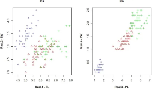
3.5.1 Iris Dataset ... 36
3.5.2 Vote Dataset ... 37
3.5.3 Heart Disease Dataset ... 37
3.5.4 Australian Credit Dataset ... 38
3.5.5 DNA-nominal Dataset ... 38
3.6 Summary ... 39
CHAPTER 4 BK INDEX FOR MIXED DATA ... 40
4.1 Motivation ... 40
4.2 Background ... 41
4.2.1 Calinski-Harabasz Index ... 41
4.2.2 Dunn Index... 42
4.2.3 Silhouette Index ... 42
4.3 Proposed Entropy-based Validity ... 43
4.3.1 Notation... 43 4.3.2 BK Index ... 44 4.3.3 Proposed Algorithm ... 45 4.4 Experiment ... 46 4.4.1 Synthetic Datasets ... 46 4.4.2 Real-world Datasets ... 49
4.4.3 Preprocessed Real Datasets... 54
4.5 Summary ... 59
CHAPTER 5 CONCLUSION ... 60
LIST OF TABLES
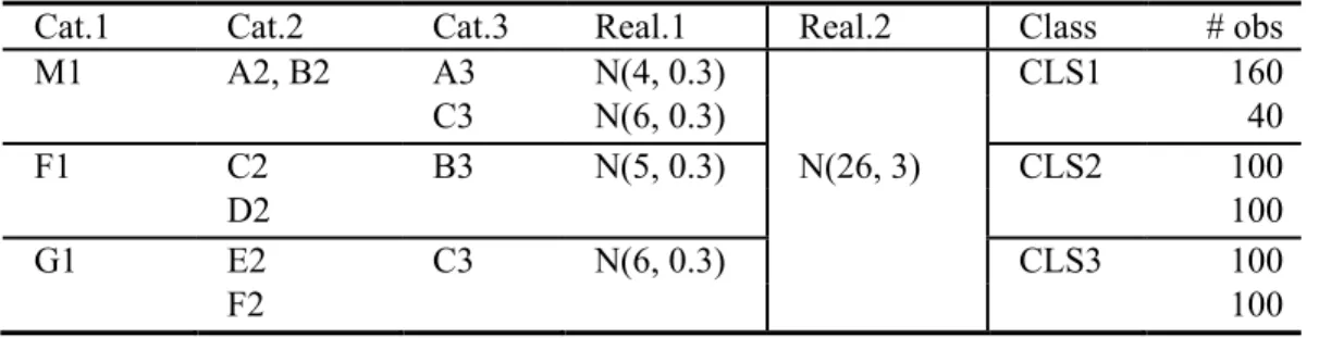
Table 1: The base dataset ds1 — three well-separated clusters. ... 27
Table 2: ds2 — co-occurrence with 20% noise. ... 27
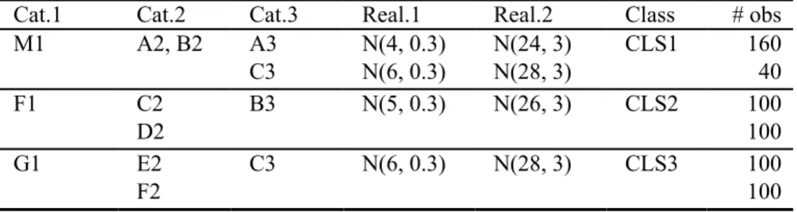
Table 3: ds5 — stronger co-occurrence with 20% noise. ... 28
Table 4: ds26 — clusters only dependent on real attributes. ... 28
Table 5: ds27 — clusters only dependent on categorical attributes... 29
Table 6: ds29 — clusters only dependent on real attributes and Cat.1. ... 29
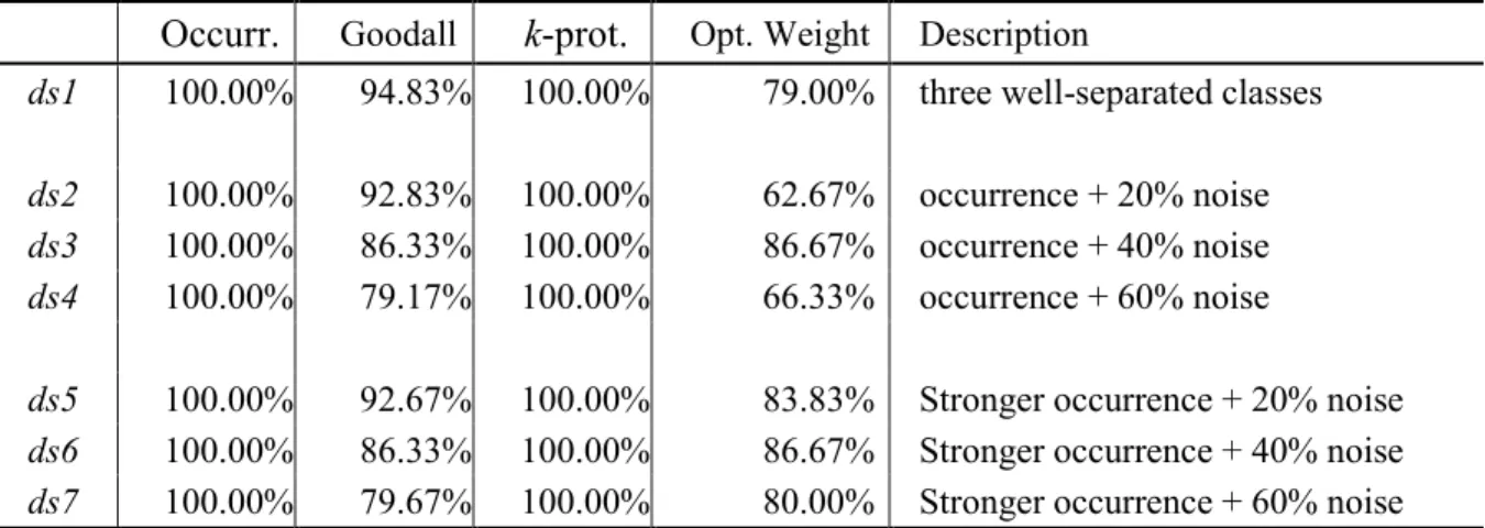
Table 7: Accuracy of synthetic datasets with co-occurrence. ... 29
Table 8: Accuracy of synthetic datasets when adding non-Gaussian noise... 30
Table 9: Accuracy of datasets with co-occurrence & nominal non-Gaussian noise. .. 30
Table 10: Accuracy of datasets with co-occurrence & real non-Gaussian noise. ... 30
Table 11: Accuracy of synthetic datasets when relaxing some attributes. ... 31
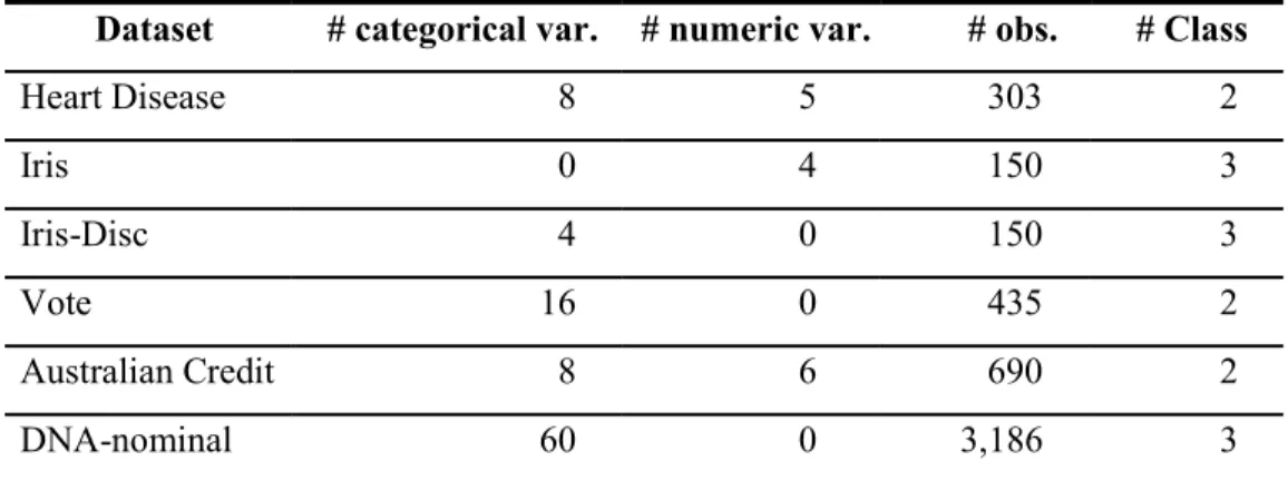
Table 12: Six real datasets from UCI. ... 32
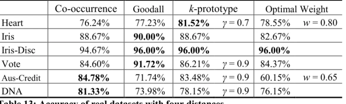
Table 13: Accuracy of real datasets with four distances... 33
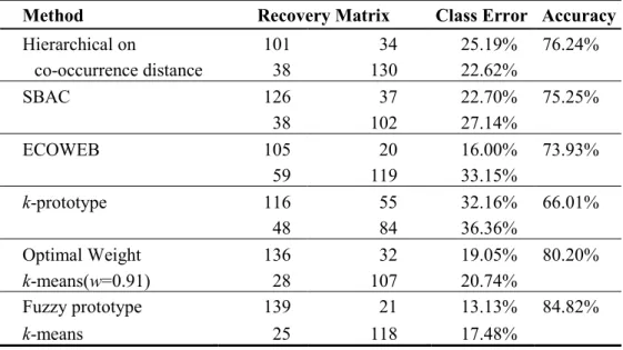
Table 14: Comparative study on Heart Disease dataset. ... 34
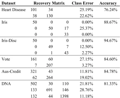
Table 15: Results of real datasets with the co-occurrence distance. ... 35
Table 16: Accuracy of preprocessed Iris dataset compared to original. ... 36
Table 17: Accuracy of preprocessed Vote dataset compared to original. ... 37
Table 18: Accuracy of preprocessed Heart Disease dataset compared to original. .... 38
Table 19: Accuracy of preprocessed Australian Credit dataset. ... 38
Table 20: Accuracy of preprocessed DNA-nominal dataset compared to original. ... 39
Table 21: Estimated numbers of clusters by four validity indices. ... 47
Table 22: Estimated numbers of clusters by four validity indices (continued). ... 48
Table 23: Estimated numbers of clusters by four validity indices for real datasets. .. 50
Table 24: Estimated numbers of clusters by four validity indices for Iris. ... 54
Table 25: Estimated numbers of clusters by four validity indices for Vote. ... 55
Table 26: Estimated numbers by four validity indices for Heart Disease. ... 56
Table 27: Estimated numbers by four validity indices for Australian Credit. ... 57
LIST OF FIGURES
Figure 1: The proposed clustering framework. ... 4
Figure 2: The scatter plots of Iris. (Left) SL vs. SW. (Right) PL vs. PW... 36
Figure 3: Plots of four indices on base dataset ds1. ... 47
Figure 4: Plots of four indices on very noisy dataset ds4. ... 48
Figure 5: B(k) for six real-world datasets. ... 50
Figure 6: Plots of four indices on Heart Disease. ... 51
Figure 7: Plots of four indices on Iris. ... 51
Figure 8: Plots of four indices on Iris-Disc. ... 52
Figure 9: Plots of four indices on Vote. ... 52
Figure 10: Plots of four indices on Australian Credit. ... 53
Figure 11: Plots of four indices on DNA. ... 53
Figure 12: Plots of four indices on Iris 2. ... 55
Figure 13: Plots of four indices on Vote 2. ... 56
Figure 14: Plots of four indices on Heart 1. ... 57
ABSTRACT
This study develops novel approaches to partition mixed data into natural groups, that is, clustering datasets containing both numeric and nominal attributes. Such data arises in many diverse applications. Our approach addresses two important issues regarding clustering mixed datasets. One is how to find the optimal number of clusters which is important because this is unknown in many applications. The other is how to group the objects “naturally” according to a suitable similarity measurement. These problems are especially difficult for the mixed datasets since they involve determining how to unify the two different
representation schemes for numeric and nominal data.
To address the issue of constructing clusters, that is, to naturally group objects, we compare the performance of four distances capable of dealing with the mixed datasets when incorporating into a classical agglomerative hierarchical clustering approach. Based on these results, we conclude that the so-called co-occurrence distance to measure the dissimilarity performs well as this distance is found to obtain good clustering results with reasonable computation, thus balancing effectiveness and efficiency.
The second important contribution of this research is to define an entropy-based validity index to validate the sequence of partitions generated by the hierarchical clustering with the co-occurrence distance. A cluster validity index called the BK index is modified for mixed data and used in conjunction with the proposed clustering algorithm. This index is compared to three well-known indices, namely, the Calinski-Harabasz index (CH), the Dunn index (DU), and the Silhouette index (SI). The results show that the modified BK index outperforms the three other indices for its ability to identify the true number of clusters.
Finally, the study also identifies the limitation of the hierarchical clustering with a co-occurrence distance, and provides some remedies to improve not only the clustering accuracy but especially the ability to correctly identify best number of classes of the mixed datasets.
CHAPTER 1
INTRODUCTION
1.1 Motivation
Clustering is one of the fundamental techniques in data mining. The primary objective of clustering is to partition a set of objects into homogeneous groups (Jain and Dubes, 1988). An effective clustering algorithm needs a suitable measure of similarity or dissimilarity, so a partition structure would be identified in the form of “natural groups”, where objects that are similar tend to fall into the same group and objects that relatively distinct tend to separate into different groups. Clustering has been extensively applied in diverse fields, including healthcare systems (Mateo et al., 2008), customer relations
management (Jing et al., 2007), manufacturing systems (Suikki et al., 2006), biotechnology (Kim et al., 2009), finance (Liao et al., 2008), and geographical information systems (Touray et al., 2010).
Many algorithms that form clusters in numeric domains have been proposed. The majority exploit inherent geometry or density. This includes classical k-means (Kaufman and Rousseew, 1990; Jing et al., 2007) and agglomerative hierarchical clustering (Day and Edelsbrunner, 1984; Yasunori et al., 2007). More recently several studies have tackled the problem of clustering and extracting from categorical data, i.e., batch self-organizing maps (Chen and Marques, 2005),matrix partitioning method (Jiau et al., 2006), k-distributions (Cai et al., 2007), and fuzzy c-means (Brouwer and Groenwold, 2010). However, while the
majority of the useful data is described by a combination of mixed features (Li and Biswas, 2002), traditional clustering algorithms are designed primarily for one data type. The
literature on clustering mixed data is still relatively sparse (Hsu et al., 2007; Ahmad and Dey, 2007; Lee and Pedrycz, 2009) and more work is needed in this area.
The main obstacle to clustering mixed data is determining how to unify the distance representation schemes for numeric and categorical data. Numeric clustering adopts distance metrics while symbolic clustering uses a counting scheme to calculate conditional probability estimates as a means for defining the relation between groups. The pragmatic methods that convert one type of attributes to the other and then apply traditional single-type clustering algorithms may lead to significant loss of information. If categorical data with a large domain
is converted to numeric data by binary encoding, more space and time are introduced. Moreover, if quantitative and binary attributes are included in the same index, these procedures will generally give the latter excessive weight (Goodall, 1966).
Apart from the need for a suitable distance measure for mixed data, another critical issue is how to evaluate clustering structures objectively and quantitatively, that is, without using the domain knowledge and expert experience. The need to estimate the number of clusters in continuous data has led to the development of a large number of what is usually called validity criteria (Halkidi et al., 2002; Kim and Ramakrishna, 2005), but there are few criteria for evaluating partitions produced from categorical clustering (Celeux and Govaert, 1991; Chen and Liu, 2009). To the best of our knowledge there is no literature that
satisfactorily addresses the cluster validation problems related to data with both discrete and real features.
The limitations of existing clustering methodologies and criterion functions in dealing with mixed data motivate us to develop clustering algorithms that can better handle both numeric and categorical attributes.
1.2 Objective
As stated above, this dissertation addresses the question of how to partition mixed data into natural groups efficiently and effectively. Later, the proposed approach will be applied to identify the “optimal” classification scheme among those partitions. The extension of clustering to a more general setting requires significant changes in algorithm techniques in several fundamental respects. To tackle the objectives stated above, the following three research tasks will therefore be addressed:
(1) We will develop an agglomerative hierarchical clustering method for clustering mixed datasets and investigate the performance of various distance measurements that represent both data types.
As mentioned above, the traditional way of converting data into a single type has many disadvantages. Within the context of an agglomerative hierarchical clustering method, we will investigate quantitative measures of similarity among objects that could keep not only the structure of categorical attributes but also relative distance of numeric values. Specifically, the measurements will be the co-occurrence distance (Ahmad and Dey, 2007),
the k-prototype distance (Huang, 1998), the optimal weight distance (Modha and Spangler, 2003), and the Goodall distance (Goodall, 1966). In the literature, the first three distances have been applied in k-means families, and the last is used in an agglomerative hierarchical clustering called the SBAC method (Li and Biswas, 2002). Our goal is to choose the distance measure that not only produces a low error rate in partitioning but is also suitable to search for the proper number of clusters.
(2) We will investigate how to determine the optimal number of classes in mixed datasets.
Evaluation of clustering structures can provide crucial insights about whether the clustering partition derived is meaningful or not. For numeric clustering, the number of clusters can be validated through geometry shape or density distribution, while cluster entropy and categorical utility are frequently used for categorical clustering. We will
investigate how to extend the extant validity indices and make them capable of handling both data types. Specifically, we will investigate two approaches since they can integrate current validation methods smoothly. First, if a quantitative distance would represent numeric and categorical dissimilarities in a compatible way, then this geometric-like distance may be exploited in traditional numeric validation methods like the Calinski-Harabasz index, in which the optimal number of clusters would be determined by minimizing the intra-cluster distance while maximizing the inter-cluster distance. Second, it is also possible to calculate the entropies of cluster structures over both components. A low entropy is desirable since it indicates an ordered structure. We claim that the increments of expected entropies of optimal clusters structures over a series of successive cluster numbers would indicate the optimal number of clusters.
(3) We will explore the property of the proposed algorithm.
There is no cure-all algorithm for clustering problems. It is important to understand which datasets would be much more applicable to be analyzed by the new algorithm. Some testing datasets with various characteristics will be generated to investigate specific
properties. Certainly, these properties could guide some data preprocessing operations on real-world datasets such as a feature selection.
1.3 Overview
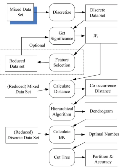
The outcome of the research is a framework that combines a hierarchical clustering integrated with a co-occurrence distance and an extension of the BK index to search for the best number of the classes. Figure 1 shows this procedure. As illustrated, it contains six main steps to recover the underlying structure of mixed datasets under the assumption that the number of classes is unknown.
Figure 1: The proposed clustering framework.
The framework works as follows: (1) calculate the significance of each attribute, in which the numeric part will be used as weights in the co-occurrence distance; (2) conduct a feature selection according to the order of attributes’ significance and the properties of the proposed algorithm. Thus, we can generate a reduced dataset that would be much more applicable to this algorithm and get better result. This step is optional, exploratory, and
iterative; (3) calculate the co-occurrence distance for the dataset of interest or the reduced mixed dataset; (4) construct a dendrogram by a hierarchical algorithm; (5) determine the optimal number of the classes by using BK index; (6) cut the tree according to this proper number and report the results.
1.4 Summary
All of the research tasks are either completely or partially new to the literature. The extended clustering applicable to arbitrary collections of datasets and the validity index for mixed datasets are particular novel and make significant contributions. The contributions in this study can be thus summarized as follows.
(1) Compare four distances capable of handling with the mixed dataset when used with hierarchical clustering.
(2) Identify limitations of the hierarchical clustering with a co-occurrence distance and propose solutions.
(3) Define a validity index to search the optimal number of clusters.
The remainder of the dissertation is organized as follows. In Chapter 2, we survey the related literature. In Chapter 3, we compare the four distances when used in an agglomerative clustering algorithm, and then choose the co-occurrence distance. The limitation of the proposed algorithm is identified. The corresponding solutions are provided. In Chapter 4, a validity index is integrated with the proposed algorithm to estimate the number of clusters for mixed data with numeric and categorical features. We conclude and suggest our future
CHAPTER 2
REVIEW OF LITERATURE
We will briefly review the literature on cluster analysis and cluster validation. The first section provides a basic understanding of clustering methods, specifically on categorical clustering and mixed clustering. Then we introduce several well-known validity indices to determine the optimal number of clusters.
2.1 Cluster Analysis
Cluster analysis was first proposed in numeric domains, where a distance is clearly defined. Then it extended to categorical data. However, much of the data in the real world contains a mixture of categorical and continuous features. As a result, the demand of cluster analysis on the mixed data is increasing.
2.1.1 Numeric Clustering
Clustering is to partition the data into groups where objects that are similar tend to fall into the same groups and objects that are relatively distinct tend to separate into different groups. Traditional clustering methodologies handle datasets with numeric attributes. The proximity measure can be defined by geometrical distance. A set of data with n objects (o1,
⋯, on) are divided into k disjoint clusters (C1, ⋯, Ck), called partition P(k). n is the number
of objects in the dataset and ni the number of objects in the ith cluster. D(Ci, Cj) is the distance
between the ith cluster and the jth cluster. d(oi, oj) is the distance between the ith object and the jth object. The centroid of the ith cluster is defined as 1
i i o C i z o n ∈ =
∑
. Z ={ ,z1 ⋯,zk}is a set of k center locations. D Z o( , i)is the shortest distance between object i and its nearest center.Clustering constructs a flat (non-hierarchical) or hierarchical partitioning of the objects. Hierarchical algorithms use the distance matrix as input and create a sequence of nested partitions, either from singleton clusters to a cluster including all individuals or vice versa. Some details on agglomerative methods are provided here since the divisive clustering is not commonly used in practice. To begin, the n objects form n singleton clusters. The clusters with the minimal distance are merged. The distances between the new generated
cluster and others will be updated according to some linkage method. The searching for two clusters with the minimal distance and the merging process continue until all objects in the same cluster. The commonly used linkage methods are listed as follows, along with the definitions of inter-cluster distances and update rules.
(1) The single linkage defines the cluster distance as the smallest distance of a pair of objects in two different clusters. It is known as the nearest neighborhood method, which tends to cause chaining effect.
, ( , ) min ( , ) i i j j i j o C o C i j D C C d o o ∈ ∈ = (2.1) ( k, ( i, j)) min( ( k, i), ( k, j)) D C C C = D C C C C (2.2)
(2) The complete linkagepicks the furthest objects in two different clusters as the cluster distance. , ( , ) max ( , ) i i j j i j i j o C o C D C C d o o ∈ ∈ = (2.3) ( k, ( i, j)) max ( ( k, i), ( k, j)) D C C C = D C C C C (2.4)
(3) The average linkageuses the average distance between all pairs of objects in cluster Ci and cluster Cj.
, 1 ( , ) ( , ) i i j j i j i j o C o C i j D C C d o o n n ∈ ∈ =
∑
(2.5) ( , ( , )) i ( , ) j ( , ) k i j k i k j i j i j n n D C C C D C C D C C n n n n = + + + (2.6)(4) The centroid linkagetakes the distance between the centroids of two clusters as the cluster distance.
( ,i j) ( ,i j) D C C =d z z (2.7) 2 ( , ( , )) ( , ) ( , ) ( , ) ( ) j i j i k i j k i k j i j i j i j i j n n n n D C C C D C C D C C D C C n n n n n n = + − + + + (2.8)
(5) The Ward’slinkage is called the minimum variance method since it uses the increment of the within-class sum of squared errors when joining clusters Ci and Cj as the
2 ( i, j) i j ( ,i j) i j n n D C C d z z n n = + (2.9) ( , ( , )) i k ( , ) j k ( , ) k ( , ) k i j k i k j i j i j k i j k i j k n n n n n D C C C D C C D C C D C C n n n n n n n n n + + = + − + + + + + + (2.10)
Non-hierarchical partition clustering employs an iterative approach to group data into a pre-specified number by minimizing a sum of weighted within-cluster distances between every object and its cluster center.
minimize 1 ( ) ( , ) n i i i f Z w D Z o = =
∑
(2.11)The weight,wi> 0, modifies the distances. If treat the weighted distance w D Z oi ( , )i as a “cost”, we formulate it as a standard discrete optimization problem.
Let xijbe a decision variable
1 if object is assigned to the cluster 0 otherwise th ij i j x =
To ensure that every object is assigned to exactly one cluster, it has
1 1 k ij j x i = = ∀
∑
The interpretation of the notation is as i : index of objects;j : index of clusters;
dij: distance between object i and the center of cluster j.
minimize 1 1 ( ) n k i ij ij i j f X w d x = = =
∑∑
(2.12) subject to 1 1 k ij j x i = = ∀∑
{0,1} , ij x ∈ ∀i jBy selecting a vector of cluster centers from the set of feasible alternatives defined by the constraints, the model achieves the minimum total cost, namely, the minimum total weighted within-group distance over all groups.
Unfortunately, this problem is NP-hard even for k = 2 (Drineas et.al, 2004). It is impossible to find exact solutions in polynomial time unless P = NP. However, there are some efficient approximate approaches, such as k-means algorithms.
2.1.2 Categorical Clustering
For categorical data which has no order relationships, conceptual clustering
algorithms based on hierarchical clustering were proposed. These algorithms use conditional probability estimates to define relations between groups. Intra-class similarity is the
probability Pr(ai = vij |Ck) and inter-class dissimilarity is the probability Pr(Ck|ai = vij), where
ai = vij is an attribute-value pair representing the ithattribute takes its jthpossible value.
Category Utility (CU) is a heuristic evaluation measure (Fisher, 1987) to guide construction of the tree in systems COBWEB (Huang and Ng, 1999) or its derivatives, e.g., COBWEB/3 (McKusick and Thomson, 1990), and ITERATE (Biswas et al., 1998). CU attempts to maximize both the probability that two objects in the same cluster have attribute values in common and the probability that objects from different clusters have different values. ROCK (Guha et al., 1999)is a clustering algorithm that works for both boolean and categorical attributes. This algorithm employs the concept of links to measure the similarity between a pair of data points. The number of links between a pair of points is the number of common neighbors shared by the points. Clusters are merged through hierarchical clustering which checks the links while merging clusters. The main objective of the algorithm is to group together objects that have more links. CACTUS (Ganti et al., 1999) is a hierarchical
algorithm to group categorical data by looking at the support of two attribute values. Support is the frequency of two values appearing in objects together. The higher the support is, the more similar the two attribute values are. The two attribute values are strongly connected if their support exceeds the expected value with the assumption of attribute-independence. This concept is extended to a set of attributes that pair wise strongly connected. Finding the co-occurrence of a set of attribute values is intensive in computational complexity.
2.1.3 Mixed Clustering
Clustering algorithms are designed for either categorical data or numeric data. However, in the real world, a majority of datasets are described by a combination of continuous and categorical features. A general method is to transform one data type to another. In most cases, nominal attributes are encoded by simple matching or binary mapping, and then clustering is performed on the new-computed numeric proximity.
Binary encoding transforms each categorical attribute to a set of binary attributes, and then encodes a categorical value to this set of binary values. Simple matching generates distance measurement in such a way that yields a difference of zero when comparing two identical categorical values, and a difference of one while comparing two distinct values. However, the coding methods have the disadvantages of (1) losing information derivable from the ordering of different values, (2) losing the structure of categorical value with different levels of similarity, (3) requiring more space and time when the domain of the categorical attribute is large, (4) ignoring the context of a pair of values, e.g., the
co-occurrence with other attributes, and (5) giving different weight to the attributes according to the number of different values they may take. Moreover, if quantitative and binary attributes are included in the same index, these procedures will generally give the latter excessive weight (Goodall, 1966).
An alternative approach is to discretize numeric values and then apply symbolic clustering algorithms. The discretization process often loses the important information especially the relative difference of two values for numeric features. In addition, it causes boundary problem when two close values near the discretization boundary may be assigned to two different ranges. Another difficult problem is to estimate the optimal intervals during discretization.
Huang (1998) extended k-modes to mixed datasets and developed k-prototype algorithm. The distances of two types of features are separately calculated. The numerical distances are measured by Euclidean distances, while the categorical distances are measured by simple matching. The centers of categorical attributes are defined as the modes in the cluster. Ahmad and Dey (2007) proposed a fuzzy prototype k-means algorithm. Similar to k -prototype, the cost function is made up of two components. The difference is that the
categorical distances are measured by the co-occurrence of two attributes and the categorical cluster centers are the lists of values in every attribute with their frequencies in the cluster. Modha and Spangler (2003) used k-means to cluster mixed datasets, but they carefully chose the weights for different features by minimizing the ratio of the between-cluster scatter matrix and the with-cluster scatter matrix of the distorted distance.
ECOWEB (Reich and Fenves, 1991) defines Category Utility measurement in
numeric attributes by approximation of the probability in some user-described interval, which has greatly impact on the performance. AUTOCLASS (Cheesman and Stutz, 1995) assumes a classical finite mixture distribution model on the data and uses a Bayesian method to maximize the posterior probability of the clustering partition model given the data. The number of classes in the data is pre-specific. The computational complexity is extremely expensive. SBAC (Li and Biswas, 2002) is a hierarchical clustering of mixed data based on Goodall similarity measurement with the assumption of attribute-independence. The distance exploits the property that a pair of the objects is closer than other pairs if it has an uncommon feature. This algorithm is computationally prohibitive and demands huge memory. Hsu and his colleagues (2007) exploited the semantics property in the domain of categorical attributes and represented each attribute with a tree structure whose leaves are the possible values of this attribute and the links associate with some user-specified weights. This hierarchical distance scheme is integrated with agglomerative hierarchical clustering and compared to binary coding and simple matching.
Some fuzzy clustering algorithms are proposed recently to attack the dataset with mixed features. Unlike hard clustering where each object belongs to only one cluster, fuzzy clustering algorithms assign each object to all of the clusters with a certain degree of membership. Yang et al. (2004) investigated symbolic dissimilarity that is originally proposed by Gowda and Diday (1991) and modified the three components parts of
dissimilarity measure. This fuzzy clustering has the strength to handle the categorical data and fuzzy data. GFCM (Lee and Pedrycz, 2009) used a fuzzy center instead of a singleton prototype for the categorical components, which took a list of partial values of a categorical attribute with their frequencies in the cluster. The size of the values in the prototype is an input parameter. Besides searching for optimal membership matrix and prototype matrix, the
algorithm has to choose a set of values from a categorical attribute domain and present them in the prototype. The size of the labels and the fuzzification coefficients affect the
performance.
2.2 Cluster Validation
Clustering algorithms expose the inherent partitions in the underlying data, while cluster validation methods are able to evaluate the result clusters quantitatively and objectively, e.g., whether the cluster structure is meaningful or just an artifact of the clustering algorithm. There are two main categories of testing criteria, known as external indices and internal indices. External indices are distinguished from internal indices by the present of priori information of known categories.
2.2.1 External Indices
Given a priori known cluster structure (P) of the data, external indices evaluate a clustering structure resulting from cluster algorithms (P′) based on counting the pairs of points on which two partitions agreement and disagreement. A pair of points can fall into one of the four cases as below:
a : number of point pairs in the same cluster in both P and P′ b : number of point pairs in the same cluster in P but not in P′ c : number of point pairs in the same cluster in P′ but not in P d : number of point pairs in different clusters under both P and P′
Wallace (1983) proposed the two asymmetric criteria W1, W2 as
W1 (P, P′) = a a+b and (2.13) W2 (P,P′)= a a+c (2.14)
representing the probability that a pair of points which are in the same cluster in P (respectively, P′) are also in the same cluster under the other clustering.
Fowlkes and Mallows (1983) took the geometric mean of the asymmetric Wallace indices and introduced a symmetric criterion
FM (P,P′) = a a .
a c a b+ + (2.15)
The Fowlkes-Mallows index assumes the two partitions are independent.
The Rand index emphasizes the probability that a pair of points in the same group or in different groups in both partitions while Jaccard’s coefficient does not take an account into ‘conjoint absence’ and only measures the portion of pairs in the same cluster.
The Rand index (Rand, 1971) R (P,P′) = a d
a b c d
+
+ + + (2.16)
The Jaccard index (Jain and Dubes, 1988) J (P,P′) = a
a b c+ + (2.17)
2.2.2 Internal Indices
Internal indices are validation measures which evaluate clustering results using only information intrinsic to the underlying data. Without true cluster labels, estimating the number of clusters, k, in a given dataset is a central task in cluster validation. Overestimation of k complicates the true clustering structure, and makes it difficult to interpret and analyze the results; on the other hand, underestimation causes the loss of information and misleads the final decision. In the following section, we will briefly review several well-known indices.
One of the oldest and most cited indices is proposed by Dunn (Dunn, 1974) to identify the clusters that are compact and well separated by maximizing the inter-cluster distance while minimizing the intra-cluster distance. The Dunn index for k clusters is defined as
1, , 1, ,
2
1, ,
( , )
* arg max ( ) min min ,
max ( ) i j i k j i k k m m k D C C k DU k diam C = = + ≥ = = = ⋯ ⋯ ⋯ (2.18)
where D(Ci, Cj) is the distance between two clusters Ci and Cj as the minimum distance
between a pair of objects in the two different clusters separately and the diameter of cluster Cm, diam(Cm), as the maximum distance between two objects in the cluster. The optimal
number of clusters is calculated at the largest value of the Dunn index. The Dunn index is sensitive to noise. By redefinitions of the cluster diameter and the cluster distance, a family of cluster validation indices is proposed (Bezdek and Pal, 1998).
Based on the ratio of the between-cluster scatter matrix (SB) and the within-cluster scatter matrix (SW), the Calinski-Harabasz index (Calinski and Harabasz, 1974) is the best among the top 30 indices ranked by Milligan and Cooper (1985). The optimal number of clusters is determined by maximizing CH(k).
( )
2 ( ) / ( 1) * arg max . ( ) / ( ) k Tr k k CH k Tr n k ≥ − = = − B W S S (2.19)Similar to the Calinski-Harabasz index, the Davies-Bouldin index (Davies and Bouldin, 1979) obtains clusters with the minimum intra-cluster distance as well as the maximum distance between cluster centroids. The minimum value of the index indicates a suitable partition for the dataset.
1, , ,
2 1
( ) ( )
1
* arg min ( ) max
( , ) k i j j k i j k i i j diam C diam C k DB k k = ≠ d z z ≥ = + = =
∑
⋯ (2.20)where the diameter of a cluster is defined as
2 1 ( ) ( , ) . i i i o C i diam C d o z n ∈ =
∑
(2.21)The Silhouette index (Kaufman and Rousseeuw, 1990) computes for each object a width depending on its membership in any cluster. For the ith object, let ai be the average
distance to other objects in its cluster and bi the minimum of the average dissimilarities
between object i and other objects in other clusters. The silhouette width is defined as (bi -
ai)/max{ai, bi}. Silhouette index is the average Silhouette width of all the data points. The
partition with the highest SI(k) is taken to be optimal.
( )
2 1 ( ) 1 * arg max max( , ) n i i k i i i b a k SI k n b a ≥ = − = = ∑
(2.22)The Geometric index (Lam and Yan, 2005) is recently proposed to accommodate data with clusters of different densities and overlap clusters. The optimal number of clusters is found by minimizing the GE(k) index. Let d be the dimensionality of the data and λpq the
eigenvalue of the covariance matrix from the data. D(Ci, Cj) is the inter-cluster distance
between cluster i and cluster j. The GE index is constructed as
2 1 1 2 1 , 2
* arg min ( ) max .
min ( , ) d ji j i k k i j j k i j k GE k D C C
λ
= ≤ ≤ ≥ ≤ ≤ ≠ = = ∑
(2.23)Unlike the criteria mentioned above, which employ the geometric-like distance, CU and entropy-based methods use the counting scheme to evaluate the performance of a categorical clustering algorithm. CU of a partition with k clusters is defined in Eq. 2.24. A cluster solution with high CU is desired since it improves the likelihood of similar patterns falling into the same cluster.
2 2 2 1 * arg max ( ) Pr( | ) Pr( ) k l i ij l i ij k l i j n k CU k a v C a v n ≥ = = = = − =
∑ ∑∑
(2.24) Entropy-based method computes the expected entropy of a partition with respect to a class attribute ai. The smaller the expected entropy, the better quality of the partition withrespect to ai. It is expected that the expected entropy decreases monotonically as the number
of clusters increases, but from some point onwards the decrease flattens remarkably. Rather than searching for the location of an “elbow” on the plot of the expected entropy versus the number of clusters, Chen and Liu (2009) calculated the second order difference of
incremental expected entropy of the partition structure, which is called the BK index. The largest value indicates an elbow point which is the potential number of clusters.
2
* arg min E ( ) Pr( | ) log Pr( | )
i l a i ij l i ij l k l j n k k a v C a v C n ≥ = = − = =
∑ ∑
(2.25)The significance test on external variables is other commonly used method. It compares the partitions using variables not used in the generation of those clusters.
Although the validity index for mixed features is relatively sparse, there are a few to evaluate fuzzy clustering algorithms based on the fuzzy partition matrices and/or
dissimilarity among objects and prototypes. For example, Lee (2009) proposed an index called CPI(k) as
2 1 1; 1; ( , ) ( , ) 1 1 * arg max ( ) ( 1) li lj i j si tj i j k k i j i j k l li lj s t s t si tj i j i j u u sim o o u u sim o o k CPI k k u u k k u u ≠ ≠ ≥ = = = ≠ ≠ ≠ = = − , −
∑
∑
∑
∑
∑
∑
(2.26)where uij is the membership of object oi in cluster j, 0 ≤ uij ≤ 1. sim(oi, oj) is any similarity
measure between object oi and oj.
2.3 Summary and Discussion
Real-life systems are overwhelmed with large mixed datasets that include numeric and nominal data. However, the majority of the clustering algorithms are designed for one data type. This study will propose a novel approach to partition mixed dataset, evaluate the resulting cluster solutions, and determine the optimal number of clusters.
CHAPTER 3
HIERARCHICAL CLUSTERING FOR MIXED DATA
Many partitioning algorithms require the number of classes, k, as a user-specified parameter. However, k is not always available in many applications. Hierarchical clustering does not need this priori information. This method creates a sequence of nested partitions. In order to form a set of clusters, a cutting point is determined by using some expert experiences to interpret each branch in the dendrogram, or by applying some validity indices to estimate where the best levels are. Our algorithm can be divided into two main procedures. First, a cluster tree is constructed by a hierarchical algorithm in a bottom up manner; and then a search procedure is followed to obtain the optimal number of classes.In this chapter, we present the first procedure that generates a cluster tree by hierarchical clustering on the distances from a co-occurrence measure. We compare four distances measurements capable of handling mixed data when used with agglomerative hierarchical clustering, and provide a solution in which the co-occurrence distance would outperform other distances. The performance is tested on some standard real-life as well as synthetic datasets.
3.1 Motivation
A distance measure that has been previously found to perform well for the fuzzy prototype k-means algorithm (Ahmad and Dey, 2007) will be adopted to define the proximity between pairs of objects. Without the assumption about data distribution, it considers the strong co-occurrence probability of two attribute values in a certain class.
Intuitively, some attribute values are associated with different classes. For example, the color of a banana is yellow while the color of a strawberry is red. If a basket has only strawberries and bananas and, by a chance, we pick a yellow fruit, then it must be a banana. Likewise, if we know the type of the fruit in this basket, then the color can be decided. Yellow and red have strong correlations with bananas and strawberries, respectively. The color of the fruit can distinguish each type of the fruit. In this context, we can assume the distance between yellow and red is large with respect to type of fruit. However, if we harvest yellow lemons and red tomatoes, and put them into this basket, then it is difficult to tell the
types of the fruits from their colors. In this situation, in terms of type of fruit, we can say a small distance between yellow and red. Therefore, a distance would be defined based on the co-occurrence of colors with respect to fruit types. A strong occurrence relationship between the two levels of color and type of fruit results in a large distance and vice versa.
Based on the power of an attribute to separate data into homogenous segments, Ahmad and Dey (2007) defined the distance between categorical attribute values and calculated the weights for numeric attributes by exploiting this co-occurrence relation. The overall distance is a sum of categorical and the weighted numeric distances and applied in the k-means algorithm to cluster mixed datasets. The comparative study showed good
performance. Ahmad and Dey’s fuzzy prototype k-means method does not work in applications without a known number of groups. Unlike Ahmad and Dey’s method, therefore, our study employs this distance in a hierarchical algorithm to derive a tree structure, which can generate a series of partitions with successive cluster numbers. These partitions will be evaluated by the validity index proposed in the following chapter. In this section, we compare the hierarchical algorithm with four distances capable of handling mixed data types in terms of clustering accuracy, and exploit the properties of the datasets would take the advantage of the co-occurrence distance when used with agglomerative hierarchical clustering.
3.2 Background
Traditional approaches of clustering datasets with mixed data types adopt distance representations by converting one type of attributes to another. One way is to transfer categorical data into numeric data by simple matching or binary coding. On the other hand, the continuous attributes are discretized into categorical data. As mentioned in the preceding chapters, these two ways are not effective in dealing with the particular mixed datasets. Some researchers have made efforts to balance numeric and nominal distances. Huang (1998) introduced a weight factor for categorical distance in his k-prototype algorithm. Modha and Spangler (2003) went further and found the optimal weight that minimizes the within-cluster weighted distance while maximizing the between-cluster weighted distance. The SBAC method (Li and Biswas, 2002) adopted the Goodall distance based on the concept that two
species are closer if they have rarer characteristics in common. From the view of probability, the Goodall distance unites categorical and numeric distances within a common framework. Ahmad and Dey (2007) defines a distance by exploiting a co-occurrence relation of values in different attributes. The k-prototype, the optimal weight, the Goodall, and the co-occurrence distances are discussed in greater details below.
3.2.1 Notation
DS(U, A) represents a set of objects in terms of their attributes, where U is a nonempty finite set of objects and A is a nonempty finite set of attributes. For example, a strawberry and a banana are two objects in U, while color, type, and weight of the fruit are the attributes in A. Let n be the number of objects and m the number of attributes. There exists a function between the set of objects and each attribute such that :
p
p a
a U→V for any ap
∈
A (p = 1, 2, …, m), i.e., ap(xi)∈Vap(i = 1, 2, …, n), xi∈
U, where Vapis called the domainof attribute ap. ap(xi) is the value of object xi on attribute ap. For example, the color of a
banana is denoted as acolor(banana) = yellow. Generally speaking, the set of attributes can be
divided into two subsets Ar and Ac according to data type, where Ar is the set of numeric
attributes and Ac the set of categorical attributes. Thus,
A
=
A
r∪
A
c. If A is the set includingcolor, type, and weight of the fruit, then Ac is the set with color and type of the fruit while Ar
contains the weight of the fruit. mrand mc are the numbers of numeric and categorical
attributes, respectively.
m m
=
r+
m
c. Given ap∈
A, x, y∈
U, if ap(x) = ap(y), then x and y aresaid to have no difference w.r.t. ap. The distance of x and y on ap is zero, denoted
by
D x y
p( , ) 0
=
when ap(x) = ap(y). For example, if one fruit in the basket is a banana andanother is a lemon, we know their colors are yellow. It can be denoted as acolor(banana) =
acolor(lemon), or
(
,
)
0
color
D
banana lemon
=
. The total distance between two objects x, y is defined as d(x, y).Let Rj = {(x, y) ∈ U
×
U: aj(x) = aj(y)}. Thus, the relation Rj partitions U into disjointsubsets according to values on attribute aj. These subsets are called equivalence classes of aj.
The equivalence class including x is Sj(x), Sj (x) = { y ∈ U : (x, y) ∈ Rj }. For example, if x
same color as the banana. Thus, Scolor(banana) is the set of all bananas and lemons in the
basket. Wj(Bj) = { Sj(x) : aj(x) ∈ Bj, Bj⊂Vap }, the set of objects whose values on aj are among
Bj. If the objects having the same value w.r.t. aj should all be included in one segment, either
Wj(Bj) or U/Wj(Bj). U/Wj(Bj) is called the simply complement of Wj(Bj), usually denoted by
~Wj(Bj). If Wcolor({yellow}) represents the set of fruits with a yellow appearance, then
~Wcolor({yellow}) is the set of fruits containing colors except yellow.
3.2.2
k
-prototype Distance
In order to cluster mixed datasets, Huang (1998) used a user-specified weight γ to balance the distance over numeric and nominal attributes and applied this measure in his k -prototype algorithm. The numeric distance is the squared-Euclidean distance; and the
categorical distance is simple matching. All numeric attributes are normalized to the range of [0, 1]. A small γ value indicates that the clustering is dominated by numeric attributes while a large γ value implies that categorical attributes dominate the clustering. Huang suggested the weight should be in the range of [0.5, 1.4]. The total distance between a pair of objects x and y is formulated as, 2 ( ) ( ) ( , ) ( , ), max( ) min( ) r i i c i i i i A a a i A a x a y d x y D x y V V γ ∈ ∈ − = + −
∑
∑
(3.1)and the computational complexity is O(mn2).
3.2.3 Optimal Weight Distance
Modha and Spangler (2003) used optimization techniques to further balance numeric and nominal distances. Instead of a user-specified weight, their method searches for an optimal weight to minimize the ratio of the within- and between-cluster weighted distances when the number of clusters is given.
The numeric features are standardized based on mean and standard deviance, and then the distance is found by taking the squared-Euclidean distance. Each categorical value is represented by a binary vector using 1-of-v encoding (v is the number of attribute values), and the distance is found by taking cosine distance. The optimal weight distance combines the weighted distances of the two data types.
2 ( ( ) ( )) ( , ) (1 ) ( , ) var( ) r i c i i i i A a i A a x a y d x y w w D x y V ∈ ∈ − = −
∑
+∑
(3.2)In order to get the optimal weight, the number of clusters should be known in
advance. Since the objective function of this minimization problem is nonlinear, it is hard to pursue an optimal solution. Modha and Spangler calculated the objective value by taking a large number in the interval [0, 1] in order to search the best one. The computational complexity is O(imn2) when choosing i iterations to search the weight.
3.2.4 Goodall Distance
Goodall (1966) proposed a similarity index based on the agreement that a pair of objects having an uncommon value of an attribute is closer than other pairs only possessing a common value among them. For example, a salmon and a bass have scales but a dolphin and a salmon have vertebra. Since there are more animals having vertebra than those having scales, a salmon is closer to a bass than to a dolphin. The author made an assumption about independent attributes. Li and Biswas (2002) adopted this distance in the SBAC method. The distance for non-identical nominal values is one, as Di(x, y) = 1, ai(x) ≠ ai(y), ai
∈
Ac. Forexample, in the case of the fruit basket, the distance between yellow and red is formulated as
D
color(
banana strawberry
,
) 1
=
. However, color( , )D banana lemon is much more complex. For a pair of identical nominal values, the distance is the sum of the possibilities of picking an identical value pair whose value is equally or more similar to the pair in question, that is, having lower or equal frequency. The formulation is as follows when s = ai(x) = ai(y), ai
∈
Ac., ( ) ( ) ( )( ( ) 1) ( , ) ( 1) ai i r V freq r freq s freq r freq r D x y n n ∈ ≤ − = −
∑
(3.3)The distance between identical numeric values is calculated as their nominal component using equation (3.3).
To calculate distance of two different numeric values, divide the domain into successive segments by the unique values of a numeric feature and count the frequency in every interval first. Sum the possibilities in a smaller range or equal-width range (l, m) but with less or equal frequency.Given s= ai(x), t= ai(y), ai(x) ≠ ai(y), ai
∈
Ar, the distance on a| | | | {| | | |, (| |) (| |)}
( )(
( ) 1)
2
( )(
( ) 1)
( , )
(
1)
(
1)
ai i r V m l t s m l t s freq m l freq t sfreq r freq r
freq l freq m
D x y
n n
n n
∈ − < − ∨ − = − − ≤ −−
−
=
+
−
−
∑
∑
(3.4)When having calculated the distances for each attribute, we use χ2 transformation to get corresponding chi-square values. The sum of these values is distributed as χ2 with the degree of freedom two times of the number of attributes. The probability of this sum is the Goodall distance of a pair of objects.
It takes O(n+vilogvi) to compute the nominal distance for a categorical attribute with
vi levels. For mc attributes, it needs mc such calls. Therefore, the running time is
O(nmc+mqclogqc), where qc = max{
i
a
V , ai
∈
Ac}. Sorting the intervals of a numeric attributewith vi unique values requires O(vi2logvi). Given lj, the number of the intervals in jth
equal-range intervals, the same-equal-range intervals are sorted by their frequencies in
2 1 ( log ) i v j j j O l l =
∑
,which is upper bounded by O v l( i2 log )l and l is the maximum number over all lj. Accordingly,
the computational complexity of numeric distances is O(nmr+mrqr2logqr+mr qr2llogl); and the
total running time is O(nm+mqclogqc+mqr2logqr+mqr2llogl), where qr is the number of
maximum number of unique values in the numeric attributes. Even in an ordinary dataset, the number of qr is huge.
3.2.5 Co-occurrence Distance
Ahmad and Dey (2007) exploit the property that if there is a stronger connection of values on ai (e.g., s and t) with different values on aj, then s and t are more powerful to
separate a dataset into pure segments w.r.t. aj. The extreme case is when s and t associate
with different values in aj.
Given Wj(Bj), let Pi(Wj(Bj)|s) be the conditional probability w.r.t. Wj(Bj) when the
value of object x on attribute ai is s, and Pi(~Wj(Bj)|s) the conditional probability of set
U/Wj(Bj) when the value of object x on attribute ai is s, where s∈Vai, ai
∈
Ac. These two(
)
i the number of , ( ) ( ) P ( ) | the number of , ( ) j j i j j i y y W B a y s W B s x x U a x s ∈ ∧ = = ∈ ∧ = (3.5)(
)
i the number of , / ( ) ( ) P ( ) | . the number of , ( ) j j i j j i y y U W B a y s W B s x x U a x s ∈ ∧ = ∼ = ∈ ∧ = (3.6)The definition of the distance of two levels in categorical attribute ai with respect to
attribute aj is
{
}
( , ) max P ( ( ) | ) P ( ( ) | ) 1.0 , j ij i j j i j j B D s t = W B s + ∼W B t − (3.7) where s, t i a V∈ , s ≠ t, ai, aj
∈
Ac. Ahmad and Dey (2007) showed an optimal solution would beobtained in polynomial algorithm in terms of
j
a
V .
The distance of two levels in categorical attribute ai is the average of Dij(s, t) over all
categorical attributes but ai. Given s = ai(x), t = ai(y), s ≠ t, ai
∈
Ac,, 1 ( , ) ( , ), 1 j c i ij j i a A c D x y D s t m ≠ ∈ = −
∑
and (3.8a) , 1 ( , ) ( , ) ( , ). 1 j c i i ij j i a A c Dist s t D x y D s t m ≠ ∈ ≡ = −∑
(3.8b)The distance between two values on numerical attribute ai
∈
Ar is( ) ( ) ( , ) , max( ) min( ) i i i i i a a a x a y D x y V V − = − (3.9)
which is equivalent to normalizing numerical attribute ai first and then taking the absolute
value of the difference.
The distance between every pair of objects w.r.t. attribute set A is defined as
2 ( ) ( ) ( , ) ( , ), max( ) min( ) r i i c i i i i i A a a i A a x a y d x y w D x y V V ∈ ∈ − = + −
∑
∑
(3.10)where wi is the weight of real attribute ai. The weight wiis introduced to modify numerical
distances based on separating power to divide the dataset into pure segments. First, a
numerical attribute ai
∈
Ar will be discretized into v intervals, where v is a predefined integer.( , ) ( , ) , ( 1) i s t i i i Dist s t w v v = −
∑
(3.11) s and t are the new assigned categorical values for discretized numerical attribute ai and vi isthe number of categorical values, vi =
i
a
V .
The running time of calculating the co-occurrence distance is O(n2m+nm2+q3m2), where q = max{
i
a
V , ai
∈
Ac}.3.3 Proposed Hierarchical Clustering Method
In this section, we will integrate an agglomerative clustering algorithm with the four distances measures capable of handling mixed datasets.
3.3.1 Agglomerative Hierarchical Algorithm
Agglomerative hierarchical algorithms start from singleton clusters and merge those clusters with minimal distances until all objects are included in one cluster. The distance between individual objects is as important in creating clusters as the cluster distance, but the cluster distance has greater weight on creating the final partition. Although there are a large number of distance definitions between a cluster and a newly formed cluster, we choose Ward’s method to minimize the increase of the within-class sum of the squared errors since we wish the formed clusters would be compact, not chain-like or with one object. The within-class sum of the squared errors is the sum of squared-Euclidean distance between each object to its nearest cluster center and is formulated as
2
i k
k i
E=
∑∑
o −z (3.12)where oi is an object in the kth cluster and zk the centroid of this cluster. If two clusters Ci and
Cj are merged, the increment of E will be calculated with the following equation: 2 . i j ij i j i j n n E z z n n ∆ = − + (3.13)
2 ( i, j) i j ( ,i j). i j n n D C C d z z n n = + (3.14)
The distance between a cluster Ck and a newly emerged cluster (Ci and Cj) is
determined by ( , ( , )) i k ( , ) j k ( , ) k ( , ), k i j k i k j i j i j k i j k i j k n n n n n D C C C D C C D C C D C C n n n n n n n n n + + = + − + + + + + + (3.15)
which would be used to update cluster distances after a merge.
The following procedure summarizes the agglomerative hierarchical algorithm. INPUT. Distance matrix for each pair of objects (x, y) ∈ (U×U).
OUTPUT. A dendrogram.
Initial: Every object forms a singleton cluster. There are n clusters.
Step 1: Search the minimal cluster distance. Assume between Cluster i and Cluster j. Step 2: Merge Cluster j into Cluster i.
Step 3: Delete the distances between Cluster j and other clusters.
Step 4: Update the distances between Cluster i and other clusters using Eq. 3.15. Step 5: Repeat Steps 2 – 4 until all objects in the same cluster.
The computational complexity for the agglomerative clustering algorithm, O(n2), is well-established in the literature (Jain and Dubes, 1988).
3.3.2 Evaluation Methodology
In the chapter on literature review, we discussed that internal criteria such as validity indices could be used to discover inherent data structures. However, in this chapter, assuming pre-classified data is provided, we can adopt an external criterion which measures the
performance of hierarchical clustering algorithms with various distances against the classes assigned a priori. Clustering accuracy is used as a main external measure of clustering results. Let ai denote the number of objects correctly assigned to the true class Ci, while bi
denotes the number of objects incorrectly assigned to the true class Ci and ci the number of
objects incorrectly rejected from the true class Ci. Clustering accuracy is defined as
1 1 . k i i d a n = =
∑
(3.16)Clustering error is defined as e = 1 – d. The error ei for class Ci is 1 – ai/n. The
precision pi and recall ri of class Ci is given by
i i i i a p a b = + and . i i i i a r a c = +
The average precision and average recall are
1 1 k i i p k
∑
= and 1 1 k i i r k∑
= , respectively. Since 1 1 ( ) ( ) k k i i i i i i a b a c n = = + = + =∑
∑
, the average precision, the average recall, and clustering accuracy are the same.3.4 Experiment
The algorithm will be tested on two kinds of datasets, synthetic and real. The use of constructed artificial datasets allows us to control their structures and facilitates investigation of which distance brings better results in which scenarios.
In order to investigate the performance of the agglomerative hierarchical algorithm integrated with four different distances, namely, the co-occurrence distance, the Goodall distance, the k-prototype distance, and the optimal weight distance, we cut the generated trees according to the priori information, the true number of clusters, and then compare the set of generated clusters with the true classes.
The weights in both the k-prototype and optimal weighted distances need to be decided. The k-prototype distance needs a user-specified weight γ to balance the nominal and numeric distances. As Huang suggested, the weight in k-prototype distance, γ, should be in the range of [0.5, 1.4]; therefore, in the experiment, γ will be set as {0.5, 0.7, 0.9, 1.1, 1.3}. We pick the solution with the highest accurate rate. What’s more, the weight w in the optimal weight distance needs intensive search in the range of [0, 1]. We therefore set w from 0 to 1 by increasing 0.05 and calculate the ratio of the within-cluster and between-cluster weighted distances given the number of clusters. The best solution is the one with the minimal ratio.