longitudinal and multilevel functional data
Huaihou Chen
Submitted in partial fulfillment of the requirements for the degree
of Doctor of Philosophy
in the Graduate School of Arts and Sciences
COLUMBIA UNIVERSITY
2012Huaihou Chen All Rights Reserved
Flexible models and methods for
longitudinal and multilevel functional data
Huaihou Chen
In the first part of this dissertation, we propose penalized spline (P-spline)-based methods for functional mixed effects models with varying coefficients. This work is motivated by a clinical study of Complicated Grief (Shear et al. 2005). In the Com-plicated Grief Study, patients receive active treatment during a treatment period and then enter a follow-up period during which they no longer receive active treat-ment. It is conceivable that the primary outcome Inventory of Complicated Grief (ICG) Scale shows different trajectories for the treatment phase and follow-up phase. The length of treatment period varies across patients, i.e., some patients stay longer in the treatment than the others, thus a model that can flexibly accommodate the subject-specific curves and predict individual outcomes is desirable. In our proposed model, we decompose the outcome into a sum of several terms: a population mean function, covariates with time-varying coefficients, functional subject-specific random effects, and a residual measurement error process. Using P-splines, we propose non-parametric estimation of the population mean function, the varying coefficient, the random subject-specific curves, the associated covariance function that represents between-subject variation, and the variance function of the residual measurement er-rors (which represents within-subject variation). The proposed methods offer flexible estimation of both the population- and subject-level curves. In addition, decompos-ing variability of the outcomes into a between- and within-subject sources is useful for identifying the dominant variance component, which in turn produces an optimal
the smoothing parameters. Furthermore, we study the asymptotic behavior of the baseline P-spline estimator. We conduct simulation studies to investigate the per-formance of the proposed methods. The benefit of the between- and within-subject covariance decomposition is illustrated through an analysis of the Berkeley growth data (Tuddenham and Snyder 1954). We identify distinct patterns in the between-and within-subject covariance functions of the children’s heights. We also apply the proposed methods to the Framingham Heart Study data.
In the second part of the dissertation, we applied a semiparametric marginal model to analyze the Northern Manhattan Study (NOMAS) data (Sacco et al. 1998). NO-MAS is a prospective, population-based study, with a goal of characterizing the func-tional status of stroke survivors following stroke. The funcfunc-tional outcome is a binary indicator of functional independence, defined by Barthel Index greater than or equal to 95. Based on generalized estimating equation (GEE) models, a previous paramet-ric analysis showed that the functional status declines over time and the trajectories of decline are different depending on insurance status. The trend in functional status may not be linear, however, which motivates our semiparametric modeling approach. In this work, we consider a partially linear model with time-varying coefficient to model the trend nonparametrically, and we include an interaction term between the nonparametric trend and the insurance variable. We consider both kernel-weighted local polynomial and regression spline approaches for estimating components of the semiparametric model, and we propose a test for the presence of the interaction effect. To evaluate the performance of the parametric model in the case of model misspeci-fication, we study the bias and efficiency of the estimators under various misspecified parametric models. We find that when the adjusted covariates are independent of time, and the link function is identity, the estimators for those covariates are asymp-totically unbiased, even if the time trend is misspecified. In general, however, under other conditions and a nonidentity link, the parametric estimators under the
mis-testing the adjusted covariates when the time trend is modeled parametrically versus nonparametrically. In the simulation studies, we observe significant gain in power of those estimators obtained from a semiparametric model compared to the parametric model when the time trend is nonlinear.
In the third part of the dissertation, we extend the semiparametric marginal model in the second part to the multilevel functional data case. This work is motivated by a clinical study of subarachnoid hemorrhage (SAH) at Columbia University, where patients undergo multiple 4-hour treatment cycles and within each treatment cycle, repeated measurements of subjects’ vital signs are recorded (Choi et al. 2012). This data has a natural multilevel structure with treatment cycles nested within subjects and measurements nested within cycles. Most literature on nonparametric analysis of such multilevel functional data focus on conditional approaches using functional mixed effects models. However, parameters obtained from the conditional models do not have direct interpretations as population average effects. When population effects are of interest, we may employ marginal regression models. In this work, we propose marginal approaches to fit multilevel functional data through penalized spline generalized estimating equation (penalized spline GEE). The procedure is effective for modeling multilevel correlated categorical outcomes as well as continuous outcomes without suffering from numerical difficulties. We provide a new variance estimator robust to misspecification of correlation structure. We investigate the large sample properties of the penalized spline GEE with multilevel continuous data and show that the asymptotics falls into two categories. In the small knots scenario, the estimated mean function is asymptotically efficient when the true correlation function is used and the asymptotic bias does not depend on the working correlation matrix. In the large knots scenario, both the asymptotic bias and variance depend on the working correlation. We propose a new method to select the smoothing parameter for marginal penalized spline regression based on an estimate of the asymptotic mean squared
parameter selector to existing alternatives such as cross validation in several settings. Finally, we apply the methods to the SAH study to evaluate a recent debate on discontinuing the use of Nimodipine in the clinical community.
Key words: Functional random effects; Generalized estimating equation; Kernel
method; Multilevel functional data; Penalized GEE; Penalized splines; Regression splines; Semiparametric longitudinal data analysis.
List of Figures vi
List of Tables viii
1 Introduction 1
1.1 Overview . . . 1
1.2 Introduction to the functional mixed-effects model . . . 2
1.3 Introduction to the semiparametric analysis of the Northern Manhat-tan Study data . . . 5
1.4 Introduction to the penalized GEE model for multilevel data . . . 8
2 A penalized spline approach to functional mixed-effects model anal-ysis 13 2.1 Overview . . . 13
2.2 Semiparametric estimation of the within-subject variation . . . 14
2.2.1 Model and proposed methods . . . 14
2.2.2 Choice of the smoothing parameters . . . 16
2.3 Functional mixed effects model and nonparametric estimation of the between-subject variation . . . 19
2.3.1 Model and proposed methods . . . 19
2.3.2 Testing the varying coefficients . . . 22
2.4.1 Preliminary . . . 23
2.4.2 Asymptotic properties for P-spline estimators with B-spline basis 25 2.4.3 Asymptotic properties for P-spline estimators with truncated polynomial basis . . . 26
2.5 Numerical results . . . 28
2.5.1 Simulation Studies . . . 28
2.5.2 Data examples . . . 32
2.6 Conclusion and discussion . . . 37
3 Semiparametric model for the functional outcome after stroke: The Northern Manhattan Study 38 3.1 Overview . . . 38
3.2 Parametric GEE . . . 39
3.3 Semiparametric model for GEE . . . 40
3.3.1 Local polynomial-based approach . . . 40
3.3.2 Regression splines-based approach . . . 41
3.4 Semiparametric model with interaction term . . . 42
3.4.1 Estimation of the semiparametric model . . . 42
3.4.2 Testing the interaction term . . . 44
3.4.3 Analysis of NOMAS data . . . 45
3.5 Bias and efficiency of the parametric estimators . . . 48
3.6 Simulation study . . . 51
3.7 Conclusion and discussion . . . 54
4 A marginal approach to reduced-rank penalized spline smoothing for multilevel data 57 4.1 Overview . . . 57
4.2 Marginal semiparametric models and reduced rank smoothing . . . . 58
4.2.2 Single-level models with categorical outcome . . . 60
4.2.3 Multilevel models . . . 61
4.3 Asymptotic properties . . . 62
4.4 Selection of the smoothing parameter . . . 65
4.5 Simulation studies . . . 66
4.6 Data analysis . . . 73
4.7 Conclusion and discussion . . . 77
Appendices 85 A. Proofs of the theorems in Chapter 2 . . . 85
B. Appendix for Chapter 3 . . . 91
C. Proofs of theorems in Chapter 4 . . . 96
Bibliography 102
List of Figures
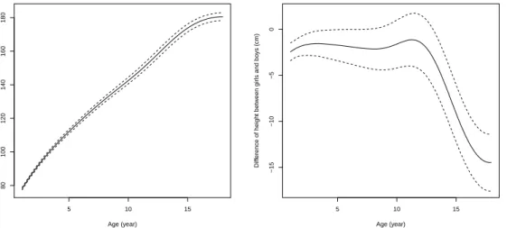
1.1 Percentage of subjects with Barthel index≥ 95 by insurance status. . 6 2.1 Estimated population mean function for boysf(t) (left panel), varying
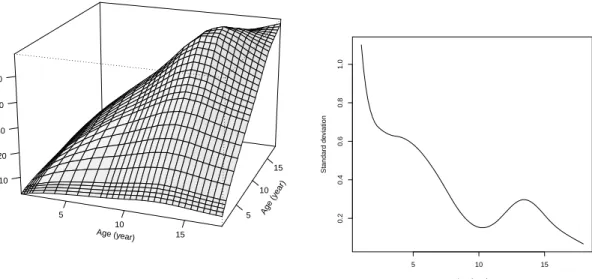
coefficient β(t) (right panel) and their 95% confidence bands. . . 33 2.2 Estimated between-subject variation γ(s, t) (left panel) and
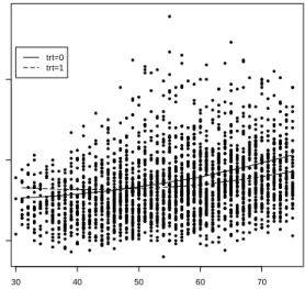
within-subject variationσ(t) (right panel). . . 34 2.3 Observed SBP values (dots) and estimated mean SBP function for
treated (f(t) +β(t), trt=1) and untreated subjects (f(t), trt=0). . . 36 2.4 Estimated between-subject variation γ(s, t) (left panel) and
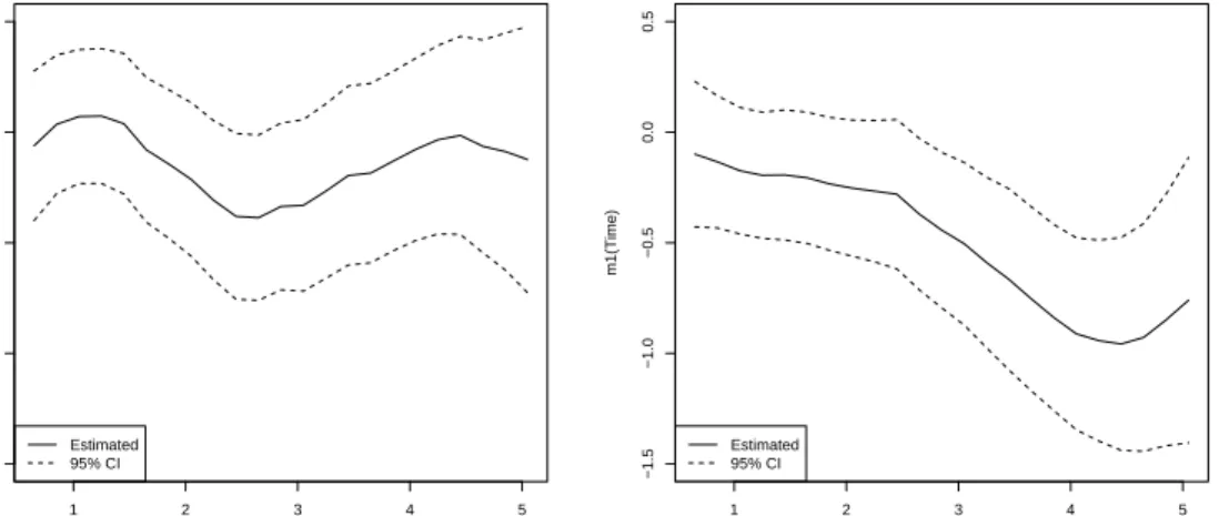
within-subject variationσ(t) (right panel). . . 36 3.1 Estimated Pr(Barthel index ≥ 95) stratified by insurance status. . . . 46 3.2 Estimated m0(t) andm1(t) and their 95% pointwise confidence bands. 46
3.3 Estimated α(t) and its 95% pointwise confidence band. . . 47 3.4 ARE of the parametric estimator ofβ. The curves from bottom to top
corresponds toρ=0, 0.1, 0.3, and 0.5. . . 50 4.1 Scatterplot of the MAP versus time measured on a subject during four
treatment cycles (dot: observed MAP; solid line: local polynomial smoothing using observed MAP in a cycle) . . . 81
at each time point; bottom left panel: assuming between-cycles inde-pendence; bottom right panel: using two-way ANOVA model based correlation structure.) . . . 82 4.3 Estimated ˆd1(t) and ˆd2(t) for MAP. (Left panel: the low dose cycles;
Right panel: the high dose cycles.) . . . 83 4.4 Estimated effect of Nimodipine on cerebral autoregulation (left panel:
the low dose cycles; right panel: the high dose cycles) . . . 83 4.5 Estimated odds ratio exp{dˆ1(t)} and exp{dˆ2(t)} of loss of
autoregu-lation. (Left panel: the low dose cycles; Right panel: the high dose cycles.) . . . 84
List of Tables
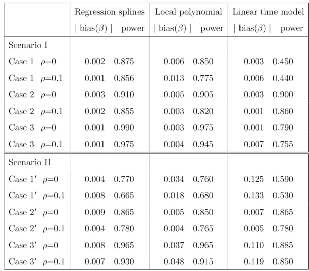
2.1 Simulation results based on model 2.1, 200 replications . . . 29 2.2 Simulation results based on model 2.5, 200 replications . . . 30 3.1 Regression coefficients in the NOMAS using the semiparametric models
and linear time model . . . 55 3.2 Semiparametric model versus linear time model, 200 replications . . . 56 4.1 Mean average MSE of fb(t) using various smoothing techniques and
smoothing parameter selectors, continuous outcome, n = 200, m = 3, 500 replications. . . 67 4.2 Pointwise standard deviation, continuous outcome, f(t) = 2 sin(2πt),
compound symmetry correlation (ρ= 0.2), normal random error, n = 200, m= 3,500 replications. . . 68 4.3 Mean average MSE of fb(t) using various smoothing techniques and
smoothing parameter selection, binary outcome, n = 100, m = 5, 500 simulations . . . 70 4.4 Pointwise standard deviation with binary outcome, exchangeable
cor-relation (ρ= 0.2), f(t) = sin(2πt),n = 100, m= 5, 500 replications. . 70 4.5 Mean average MSE of fb(t) and SE of ˆβ using different correlation
structures, continuous outcome, multilevel model, 500 replications. . . 71 4.6 Pointwise standard deviation, continuous outcome, multilevel model,
normal random error, 500 replications. . . 79
structures, binary outcome, multilevel model, 500 replications. . . 80 4.8 Pointwise standard deviation, binary outcome, multilevel model, 500
replications. . . 80
Acknowledgments
This project would not have been possible without the support of many people. Many thanks to my advisers, Professor Myunghee Cho Paik and Professor Yuanjia Wang, for their invaluable guidance and comments while this work being conducted. Also thanks to my committee members, Professor Ian McKeague, Professor Naihua Duan and Professor Mitchell S. V. Elkind, who offered guidance and support. Thanks to Dr. Elkind for providing the The Northern Manhattan Study data. Thanks to H. Alex Choi for providing the Nimodipine data. Thanks to all my classmates at Columbia University and my friends for their support and help. Finally, thanks to my parents, and my wife Xiaoyi An for their understanding and endless love, through the duration of my studies.
Chapter 1
Introduction
1.1
Overview
This dissertation develops several new methods for semiparametric analysis of longi-tudinal data and multilevel functional data. The dissertation consists of three parts. In the first part of (Chapter 2), we propose flexible functional mixed-effects models as conditional approaches for the analysis of longitudinal or functional data. The proposed methods offer flexible estimation of both the population- and subject-level curves. In the second and third parts (Chapters 3 and 4), we propose marginal semiparametric generalized estimating equation (GEE) models and methods for the analysis of single-level and multilevel functional data. In Chapter 3, we consider a partially linear model with a varying coefficient function. We use both kernel weighted local polynomial and regression splines approaches for estimating the components in the semiparametric model, and propose a test for the presence of the interaction ef-fect. In Chapter 4, we propose marginal approaches to fit multilevel functional data through penalized splines. In contrast to Chapter 2, here we are interested in pop-ulation averaged marginal means. Since the procedure only requires specification of the first two moments, it is particularly effective for modeling multilevel categorical outcomes and does not suffer from numerical difficulties.
1.2
Introduction to the functional mixed-effects
model
Repeated measurements are routinely collected in biomedical research studies. Com-prehensive reviews of parametric methods for analyzing repeated measurements data can be found in Diggle et al. (2002) or Fitzmaurice et al. (2004). In some applications, concerns on model misspecification for parametric methods may call for more flex-ible nonparametric or semiparametric approaches. Functional mixed effects models are suitable tools to accommodate flexible population mean curves and subject-level curves. For example, in many clinical studies, patients receive active treatment dur-ing a treatment period and then enter a follow-up period durdur-ing which they no longer receive active treatment. Taking the Complicated Grief Study (Shear et al. 2005) as an example, patients in the study are randomly assigned to either an interpersonal psychotherapy or a complicated grief treatment in 16 sessions over a 16- to 20-week treatment period. In addition to the treatment sessions, there is a 6-month follow-up period. For each patient, their Inventory of Complicated Grief (ICG) Scale, a 19-item self-report instrument that assesses symptoms of complicated grief, are obtained over the treatment and follow-up periods. It is conceivable that the primary outcome, ICG, shows different trajectories for the treatment phase and follow-up phase. Since each patient received a different length of treatment ranging from 16 to 20 weeks, a flex-ible model that can accommodate the subject-specific curves and predict individual outcomes is desirable.
In other applications, in addition to modeling a mean function, modeling a covari-ance function of the subject-specific processes is of scientific interest. For example, in genetic studies such as the Framingham Heart Study, the covariance of related sub-jects within a family represents genetic information. This function is used to compute heritability (ratio of genetic variance and total trait variance) which quantifies the genetic effect on a trait (Khoury et al. 1993). In some applications, although not
of direct scientific interest, accurate estimation of a covariance function leads to effi-ciency gain in estimating population mean function and fixed effects parameters (Fan et al. 2007).
In the context of longitudinal data analysis, Diggle and Verbyla (1998) pro-vided nonparametric estimation of covariance structure by using local polynomials to smooth various moment estimators of the variance and covariance functions. Wu and Pourahmadi (2003) and Huang et al. (2006) proposed nonparametric estimators for large covariance matrix via Cholesky decomposition for balanced data, which are guaranteed to be positive definite. In the context of functional data analysis, Guo (2002) considered functional mixed effects models and introduced a Kalman filtering algorithm to handle large matrices in the mixed model representation of smoothing splines which may be computationally challenging. Krafty et al. (2008) dealt with a varying coefficient model and pursued a smoothing spline based approach with an it-eratively reweighted least square procedure to fit the model. Rice and Wu (2001) used regression spline based methods and treated subject-specific curves to be nonparamet-ric random curves. Fan et al. (2007) proposed a semiparametnonparamet-ric method to estimate the error covariance function where the variance function is modeled nonparametri-cally with local polynomials and the correlation function is modeled parametrinonparametri-cally. To alleviate computational burden, Durban et al. (2005) pursued a simple penalized spline (P-spline, Eliers and Marx 1996) based approach to fit subject-specific curves which expressing these curves as a linear combination of truncated polynomial spline basis with random coefficients and specified a simplified parametric covariance matrix for the basis coefficients.
In the first part of the dissertation (Chapter 2), we present general models that decompose longitudinal outcome as a sum of several terms: a baseline mean function, covariates with time-varying coefficient, random subject-specific curves and a residual measurement error process. Using penalized splines, we propose nonparametric esti-mation of the baseline function, the varying coefficient, the subject-specific curves and
the associated covariance function which represents between-subject variation, and the variance function of the residual measurement errors (which represents within-subject variation). Decomposing variability of the outcomes as a between-within-subject source and a within-subject source is useful in identifying the dominant variance component, which in turn produces an optimal model for the covariance function. The benefit of such decomposition is illustrated through an analysis of the Berke-ley growth data (Tuddenham and Snyder 1954), where we identify clearly distinct patterns of the between- and within-subject covariance. Both covariance function estimations proposed here satisfy the positive semidefinite constraint.
All nonparametric components of our model are estimated through P-splines, which is considered as a reduced rank smoother. P-spline was originally proposed by O’Sullivan (1986) and has gained popularity since publications of Eilers and Marx (1996) and Ruppert, Wand, and Carroll (2003). A comprehensive review of penal-ized splines can be found in Ruppert et al. (2003, 2009). The number of knots in a penalized spline smoothing is usually less than the sample size which may lead to computational advantage in estimating a covariance function and subject-specific curves. More specifically, through the mixed effects model representation of a penal-ized spline expansion of the random subject-specific curves, one would notice that the dimensionality of the covariance matrix of the random basis functions is reduced due to moderate number of knots. Theoretical work has shown that penalized spline as a low rank approximation can be asymptotically as efficient as as full rank estimators such as smoothing splines (Li and Ruppert 2008; Claeskens et al. 2009).
Current literature studies the asymptotic properties of penalized spline estima-tor obtained from univariate data (a single measurement for each subject). Li and Ruppert (2008) examined the asymptotics of a P-spline estimator with B-spine basis and first or second order penalty assuming the number of knots is relatively large. Kauermann et al. (2009) studied the P-spline estimator with generalized non-normal outcomes. Claeskens et al. (2009) obtained two asymptotic scenarios of the P-spline
estimator and showed the asymptotic bias and variance for each scenario with univari-ate data. In the first part of this dissertation, we examine the asymptotic properties of the P-spline nonparametric baseline function estimated with longitudinal data. We show that under appropriate assumptions, the order of the bias and the variance term is the same as for the univariate data as shown in Claeskens et al. (2009).
Chapter 2 is structured as follows. Section 2.2 proposes methods to estimate the within-subject covariance function semiparametrically, and introduces likelihood based methods to choose smoothing parameters. Section 2.3 develops methods for a wider class of partially linear model with varying coefficients, random subject-specific curves and heteroscedastic measurement errors. In Section 2.4, we show the asymptotic bias, variance and normality of the penalized spline estimator with balanced data. In Section 2.5, we conduct two simulation studies to investigate performance of the proposed methods and apply them to analyze the Berkeley growth data and the Framingham Heart Study data. In Section 2.6, we summarize our findings and discuss possible extensions.
1.3
Introduction to the semiparametric analysis of
the Northern Manhattan Study data
In the second part of this dissertation (Chapter 3), we applied a semiparametric model with interaction term to analyze the Northern Manhattan Study (NOMAS) data. The NOMAS includes a population-based, prospective incident ischemic stroke follow-up study, which is designed to determine stroke incidence, outcomes, and risk factors in a multiethnic urban population (Sacco et al. 1998). One of the goals of NOMAS is to characterize the functional status of stroke survivors over time after stroke. All patients enrolled in the study were scheduled to have semi-annual follow up visits for the first two years after stroke, then annually until 5 years of follow-up. Dhamoon et al. (2009) analyzed functional outcomes among 379 subjects after stroke
in the NOMAS cohort. The outcome is a binary indicator of functional independence, defined by Barthel Index greater than or equal to 95. Based on Generalized Estimat-ing Equation (GEE) models, Dhamoon et al. (2009) reported that functional status declines over time, and the trajectories are different depending on insurance status, adjusting for demographics and known risk factors. In addition, we noted that the time trends may not be linear. Figure 1.1 shows that time trends for the two groups defined by insurance status are different.
Figure 1.1: Percentage of subjects with Barthel index ≥95 by insurance status.
1 2 3 4 5 0 10 20 30 40 50 60
Year after stroke
Percentage of subjects with Barthel >=95
● ● ● ● ● ● ●
Medicare or private insurance Medicaid or uninsured
In practice, parametric models are parsimonious and useful. However, they may not be sufficient in describing the relationship between the outcome variable and the covariates. Misspecification of the time trend could result in bias and inefficiency of coefficient estimates for other covariates in a model. Semiparametric models re-late the outcome variable with some covariates parametrically and other covariates nonparametrically, hence semiparametric models keep the flexibility of the nonpara-metric models for the time trend, and retain the parsimonious property of paranonpara-metric models as well. Lin and Carroll (2001) proposed a semiparametric model along with the kernel weighted local polynomial method for estimation. They showed that the estimator using working independence is quite efficient. However, in practice, when
the within-subject correlation is strong, it will be less efficient if one uses working independence (Wang 2003). Three more efficient approaches have been proposed: Wang et al. (2005), Chen and Jin (2006) and Huang et al. (2007). The method in Wang et al. (2005) involved residuals from an initial model, for example, the working independence model in Lin and Carroll (2001), therefore, it is computationally in-tensive to be implemented. Chen and Jin (2006), used piecewise local polynomial to approximate the unknown function, obtained consistent estimator for the parametric part, and then used backfitting to obtain a smooth estimator for the unknown func-tion. Alternatively, Huang et al. (2007) applied regression splines to approximate the unknown function, and obtained a smooth fit for the nonparametric function and con-sistent estimators for the parametric part simultaneously. When the within-subject correlation is strong, all the three aforementioned methods are more efficient than the one in Lin and Carroll (2001). Among the three methods, Huang et al.(2007) is easier to implement than the other two.
One of our goals is to apply a semiparametric model to reanalyze functional out-come data after stroke to better understand the trajectory after stroke and to effi-ciently estimate the covariates. Since Figure 1.1 shows that the trajectories of the two insurance groups are different, we need to distinguish the two functions in the semi-parametric model. First, we consider an extension of the method in Lin and Carroll (2001) by allowing an interaction term between the nonparametric time trend and an indicator variable. We show the asymptotic properties of the estimators and propose a statistic to test the interaction term between the time trend and a covariate. We also consider the regression spline-based method in Huang et al. (2007) and extend the model to the time-varying coefficient model.
Another goal is to evaluate bias and efficiency of parametric model in case of model misspecification. Specifically, we investigate the bias of the estimators from a possibly misspecified parametric model. We identify conditions for the misspecified time trend to still result in unbiased estimator of the covariates and compare their efficiency to
the regression splines-based estimators. We find that when the adjusted covariates are independent of the time, and the link function is identity, the estimators for the covariates are asymptotically unbiased, even if the unknown function is misspecified. In general, however, under other conditions and non-identity link, the parametric estimators are biased and less efficient even when they are unbiased. This gives an important message in designing and executing studies in that if measurements are taken in a balanced way between the treatment or exposure groups, the resulting modeling will be robust against misspecification.
The structure of Chapter 3 is as follows. Sections 3.2 and 3.3 respectively review the parametric and semiparametric GEE methods for longitudinal data analysis. Sec-tion 3.4 presents the semiparametric model with an interacSec-tion term, i.e., the time-varying coefficient model, the algorithm for estimation, and a statistic for testing no interaction. We also show the semiparametric analysis results for the NOMAS data in Section 3.4. In Section 3.5, we study the bias of the estimators from misspecified parametric model and compare the efficiency with the regression splines-based esti-mators when misspecified parametric models give consistent estiesti-mators. In Section 3.6, we conduct simulation studies to compare the semiparametric methods with the parametric method in terms of power for testing the adjusted covariates. Discussions follow in Section 3.7.
1.4
Introduction to the penalized GEE model for
multilevel data
In the third part of the dissertation (Chapter 4), we extend the semiparametric marginal model in the second part to the multilevel functional data case. Multi-level functional data is often collected in many biomedical studies. For example, in the study of the effect of Nimodipine on patients diagnosed with subarachnoid hem-orrhage (SAH) at Columbia University, each patient is administered with one of the
two doses of Nimodipine during multiple 4-hour treatment cycles (Choi et al. 2012). Subarachnoid hemorrhage (SAH) is an acute cerebrovascular event caused by rup-ture of a cerebral aneurysm. It can have devastating consequences, causing serious morbidity and mortality. Nimodipine is the only medication shown in phase III tri-als to improve clinical outcomes after SAH (Dorhout et al. 2007). Although initial clinical studies did not document low blood pressure as a side effect, during routine clinical usage a decrease in the blood pressure and even a decrease in brain oxygen delivery has been observed (Stiefel et al. 2004). Given these more recent findings and observations from clinical experience, the clinical utility of Nimodipine has been challenged and recent clinical guidelines have suggested discontinuing the use of Ni-modipine if it is associated with significant decreases in blood pressure. Although this is a strong recommendation, the committee admits to little clinical data supporting their recommendation (Dringer et al. 2011).
Nimodipine is administered to patients with SAH at one of the two doses every 4 hours, creating multiple 4-hour treatment cycles. Within each treatment cycle, subjects’ vital signs such as mean arterial blood pressure (MAP) and brain tissue oxygenation are recorded continuously and averaged over 10 minutes. Every 4 hours a patient receives a high dose or a low dose of Nimodipine depending on his or her clinical profile. This scenario creates a natural multilevel data structure with treatment cycles nested within subjects and repeated outcome measurements nested within cycles. Our primary research interest is to estimate mean physiologic outcomes averaged across treatment cycles and across subjects to evaluate the acute effects of Nimodipine on systemic and brain physiology. Specific research questions include whether Nimodipine increases or reduces the MAP and its effect on the risk of cerebral autoregulation loss.
Modeling multilevel functional data has received extensive attention recently. Brumback and Rice (1998) used smoothing splines based methods to analyze multi-level nested samples of functional data. Zhou et al. (2008) proposed jointly modeling
of paired sparse functional data by reduced rank principal components. Baladan-dayuthapani et al. (2008) and Staicu et al. (2010) developed functional mixed effects model based Bayesian approaches for correlated multilevel spatial data. Apanasovich et al. (2008) proposed composite likelihood based approach for correlated binary data. Di et al. (2009) developed functional multivariate analysis of variance which used a few functional principal components to reduce dimensionality. Greven et al. (2010) proposed a computationally efficient functional principal components analysis appli-cable to functional data observed at multiple time points.
The above methods on multilevel functional data in the current literature focus on conditional approaches through a functional mixed effects model or functional principal components analysis. In clinical trials, such as the SAH study (Choi et al. 2012), the goal is to estimate the population average effect or group difference. To achieve this goal, marginal approaches are more suitable than conditional approaches. There is a wealth of literature on nonparametric marginal regression models through local polynomial or kernel based methods (see for example, Lin and Carroll 2000, Welsh et al. 2002, Lin et al. 2004). In particular, Welsh et al. (2002) compared the efficiency of the local kernel based methods with spline based methods for marginal models with single-level functional data. However, it is not straightforward to apply kernel smoothing to accommodate the multilevel data structure. A few other works that propose marginal models fitted by smoothing splines include Ibrahim and Su-liadi (2010a, 2010b). In a variable selection setting, Fu (2003) proposed penalized generalized estimating equation (penalized spline GEE) to handle collinearity among variables.
The pros and cons of marginal versus conditional model for longitudinal data has been debated extensively in literature (see for example, Diggles et al. 2002). Marginal models provide a direct estimation of the population average effect. In contrast, for categorical outcomes, conditional models do not directly give estimators of popula-tion averaged marginal effects due to a non-identity link funcpopula-tion. Therefore, when
marginal effects are of interest, subject-specific random effects need to be integrated out, usually through numerical integration. In addition, a potential computational advantage of the marginal regression is that since the procedure only requires the specification of the first two moments of the marginal distribution, it is particularly effective for modeling correlated categorical outcomes. Numerical algorithms for con-ditional approaches for multilevel functional data with categorical outcomes may not always converge. In the SAH study, the functional mixed effects model with a two-level random effects did not converge for the primary binary outcome. Furthermore, a widely known advantage of using a robust sandwich variance estimator in marginal models is that it remains consistent under a misspecified working correlation struc-ture. For a parametric model, the estimated mean parameters are asymptotically efficient when the true correlation is used. However, for nonparametric models fit-ted by local polynomials, such property does not hold (Lin and Carroll 2000). To take into account the within-cluster correlation to improve efficiency, seemingly un-related kernel estimator should be used (Wang 2003, Lin et al. 2004). It may not be straightforward to adapt local kernel based approaches to effectively account for more complicated multilevel functional data.
There is few literature on marginal approaches for multilevel functional data through reduced-rank penalized spline smoothing (P-spline; Eilers and Marx 1996; Ruppert et al. 2003). In this work, we study semiparametric marginal models for multilevel functional data through reduced-rank penalized spline smoothing. These methods provide tools to evaluate population average effect for categorical outcomes without integrating over distribution of random effects. We investigate large sam-ple properties of the proposed estimator and show that similar to the asymptotic results in Chapter 2, the asymptotics falls into two scenarios. For the small knots scenario, the estimated mean function is asymptotically efficient when the true cor-relation function is used, and the asymptotic bias does not depend on the working correlation matrix. In contrast, for the large knots scenario, both the asymptotic bias
and variance depend on the working correlation. A practical use of the asymptotic results is to develop a new method for selecting the smoothing parameter based on an estimated asymptotic mean squared error (MSE). Simulation studies suggest superior performance compared to existing alternatives such as cross validation or generalized cross validation.
The structure of Chapter 4 is as follows. Section 4.2 studies semiparametric marginal models for single-level and multilevel functional data. Section 4.3 inves-tigates large sample properties of the proposed estimator. Section 4.4 proposes a new method to select the smoothing parameter based on an estimate of the asymptotic mean squared error (MSE). In Section 4.5, we conduct simulation studies to evaluate the performance of the proposed methods. In Section 4.6, we apply the proposed methods to the study of Nimodipine on patients with SAH. Finally, in Section 4.7 we summarize our findings and discuss some possible extensions of the work.
Chapter 2
A penalized spline approach to
functional mixed-effects model
analysis
2.1
Overview
In this chapter, we propose flexible functional mixed-effects models as conditional approaches for the analysis of longitudinal or functional data. The proposed methods offer flexible estimation of both the population- and subject-level curves. In the first section, we propose methods to estimate the within-subject covariance function semi-parametrically and introduce likelihood based methods to choose smoothing param-eters. In the second section, we develop methods for a wider class of partially linear model with varying coefficients, random subject-specific curves and heteroscedastic measurement errors. In the third section, we show the asymptotic bias, variance and normality of the penalized spline estimator with balanced data. In the fourth section, we conduct two simulation studies to investigate performance of the proposed meth-ods and apply them to analyze the Berkeley growth data and the Framingham Heart Study data. Finally, we summarize our findings and discuss possible extensions in
the fifth section.
2.2
Semiparametric estimation of the within-subject
variation
2.2.1
Model and proposed methods
In this section we first propose methods to account for the within-subject het-eroscedastic errors while estimating the mean function nonparametrically. In the next section, we propose a wider class of models to accommodate covariates with varying coefficients functions and functional subject-specific random effects. Consider a par-tially linear model,
Yij =f(Tij) +XijTβ0+ZijTbi+ij, i= 1,· · · , n, j = 1,· · · , mi, (2.1) where f(t) is a nonparametric baseline function, Tij is the design time point, Xij is a px ×1 vector of covariates and β0 is the associated parameter vector, bi are i.i.d. random effect vectors following N(0, D), Zij are the associated design vectors, n is the number of subjects, and mi is the number of repeated measurements for subject i. The measurement errorsi = (i1,· · · , imi)
T are assumed to be independent of the random effects and follow
i ∼N(0, V 1 2 i Ri(ρ)V 1 2 i ), (2.2)
where Vi = diag{σ2(Ti1),· · · , σ2(Ti,mi)} is the variance function which will be
mod-eled nonparametrically and Ri(ρ) is a parametric correlation matrix such as AR-1 or compound symmetry with ρ as the unknown vector of parameters. In practice the parametric form of the mean function and the covariance function may be un-known. For example, the Berkeley growth data which we analyzed in Section 2.5.2 clearly illustrates a non-linear trend of the mean function and the variance function of children’s heights which are not straightforward to model parametrically. The Fram-ingham data in Section 2.5.2 also shows features that may be missed if one specifies
an incorrect parametric model. It is well known that when a parametric model is misspecified, the model-based inferences are invalid. Therefore it is useful to examine more flexible nonparametric or semiparametric models.
Define the pth order truncated polynomial spline base
B(t) = {1, t,· · · , tp,(t−τ1)+p,· · · ,(t−τK)p+}, (2.3)
where τ1,· · · , τK are K knots.
Assume that the mean and the residual variance function can be approximated by
f(t)≈B(t)βf, log{σ2(t)} ≈B(t)η,
where B(t) is a row vector of basis functions and βf and η are the associated coef-ficients for the mean and the variance function. The heteroscedastic variance of the residual errors can be expressed as
Vi = diag{exp(B(Tij)η)}j=1,···,mi.
With the above notation, we can rewrite the model (2.1) as Yi =Xiβ+Zibi+i, whereYi = (Yij)j=1,···,mi,Bi ={B T(T i1),· · · , BT(Timi)} T,X i ={(Xi1,· · · , Ximi) T, B i}, β = (βT 0, βfT)T, and Zi = (Zi1,· · · , Zimi) T. Denote Y∗ i = Yi −Xiβ−Zibi, we define the penalized log-likelihood as
lp = n X i=1 {log|V 1 2 i RiV 1 2 i |+Y ∗ i T (V 1 2 i RiV 1 2 i ) −1Y∗ i }+λfβfTP βf +λσηTP η, (2.4) where λf and λσ are smoothing parameters for the mean and the variance function and P is penalty matrix depending on the chosen basis. For example, for the p-th order truncated polynomial basis with K knots, P = diag{0p+1,1K} which implies that (2.4) only penalizes the spline coefficients. Throughout this section, we use truncated polynomial basis.
For given variance components, we estimate the baseline function by minimizing lp in (2.4) and the solution takes the form of a ridge estimator as
b β = ( n X i=1 XiTΣ−i 1Xi+λfdiag{0px, P}) −1 n X i=1 XiTΣ−i 1Yi, where Σi =ZiDZiT +V 1 2 i RiV 1 2
i . To estimate the covariance matrix of the parametric random effectsD, we use the EM algorithm. To fit the variance function of the within-subject residual measurement error, since no explicit solution exists for minimizing lp with respect to η, we use the Newton-Raphson algorithm. To be specific, we obtain
b η iteratively by b η(k+1) =ηb(k)− ∂2l p ∂η∂ηT|ηb (k) −1 ∂lp ∂η |ηb (k) ,
where k index an iteration of the algorithm, and the first and the second derivatives are easily obtained based on (2.4). The correlation parameters ρ are obtained by minimizing lp also through a Newton-Raphson algorithm when no explicit solution exists.
2.2.2
Choice of the smoothing parameters
The smoothing parameters play a crucial role in the estimation procedure. Too small a penalty will lead to wiggly curves, while too large a penalty will result in flat polynomial curves which may lose the characteristic of the functions. Wand (2003) showed that by specifying spline coefficients of truncated polynomial basis functions as random effects in a linear mixed effects model, the penalized spline estimate with the smoothing parameter taken as the ratio of two variance components is identical to the best linear unbiased predictor (BLUP) obtained from a mixed effects model. Krivobokova and Kauermann (2007) showed that using the restricted maximized like-lihood (REML) to estimate smoothing parameter outperforms other methods such as (generalized) cross-validation or the Akaike information criterion especially when the error correlation structure is misspecified. Krivobokova et al. (2008) formulated a
hierarchical mixed model to estimate local smoothing parameter to achieve adaptive penalized spline smoothing. Kauermann and Wegener (2011) proposed to view the smoothing parameter of a variance function as a parameter and estimate it via max-imizing the marginal log-likelihood. Here we use a similar likelihood-based strategy to chose λf and λσ.
Denote X = (X1T,· · · , XnT)T = (X(1), X(2)) where X(1) is the first px +p + 1
columns of X and X(2) is the remaining K columns, where px is the length of the vector Xij. Denote β = (β1T, β2T)T as the associated parameter vector. Due to the link of penalized spline likelihood and mixed effect models, we can treat the spline coefficients β2 as random effects following N(0, σ2β2I) (Wand 2003; Krivobokova and
Kauermann 2007). Integrating out the random components bi, i = 1,· · · , n, and β2
results in the marginal likelihood. The smoothing parameter can be obtained via maximizing the marginal restricted log-likelihood
lm(λf) =−1 2log|Σ| − 1 2(Y −X(1)β1) T Σ−1(Y −X(1)β1)− 1 2log|X T (1)Σ −1 X(1)|,
where Σis the marginal covariance of Y, i.e.,
Σ = E{V ar(Y|b, β2)}+V ar{E(Y|b, β2)} = V +Zdiag{D,· · · , D}ZT + 1 λf X(2)X(2)T , with V = diag{V 1 2 1 R1V 1 2 1 ,· · · , V 1 2 n RnV 1 2
n}. Note that here the smoothing parameter λf appears as a parameter in the covariance matrix Σ. Applying Newton-Raphson algorithm, we have λ?f(k+1) =λ?f(k)− ∂ 2l m(λf) ∂λ?2 f |λ∗f(k) !−1 ∂lm(λf) ∂λ? f |λ∗f(k) ! ,
where λ?f = 1/λf. The first and the second derivatives are easy to obtain. Finally, we obtainλbf = 1/bλ?f.
We use a similar strategy to choose the smoothing parameter λσ of the variance function. To be specific, regard the spline coefficients in η as random effects and
integrate them out to obtain the marginal log-likelihood lm(λσ) = log Z expn− 1 2 n X i=1 (log|V 1 2 i RiV 1 2 i |+Y ∗ i T (V 1 2 i RiV 1 2 i ) −1Y∗ i ) − 1 2λση T P η+1 2log|λσP|+ o dη.
Since there is no explicit solution to such an integration, we apply Laplace approxi-mation to obtain lm(λσ) ≈ − 1 2 n X i=1 {log|V 1 2 i RiV 1 2 i |+Y ∗ i T (V 1 2 i RiV 1 2 i ) −1Y∗ i } − 1 2λση TP η− 1 2log|H|+ 1 2log|λσP|+, withH =−∂ 2(−1 2lp) ∂η∂ηT = 1 2 ∂2lp
∂η∂ηT.Laplace approximation of a likelihood function has been discussed in Wolfinger (1993) and Kauermann and Wegener (2011). Specifically, we can approximate the marginal log-likelihood function
log Z exp{l(η)}dη≈l(bη)− 1 2log| −l 00 (η)b|+const.
The above approximation has an error of order O(1/n). One important condition to achieve this approximation rate is that the number of spline bases functions must be small compared to the sample sizen, that is, K n (Severini 2000; Kauermann and Wegener (2011)). This condition is satisfied by penalized spline smoothing since the number of knots is much smaller than the sample size. Denote the right hand side of the above display as ˜lm(λσ) and set its first derivative with respect toλσ to zero, i.e.,
∂˜lm(λσ) ∂λσ =−1 2ηb TP b η−1 2tr{H −1P}+ Kσ 2λσ = 0, yields b λσ = 1 Kσ (bηTPbη+tr{H−1P}).
2.3
Functional mixed effects model and
nonpara-metric estimation of the between-subject
vari-ation
2.3.1
Model and proposed methods
In this section, we propose methods for a wider class of functional mixed effects models where we accommodate covariates with varying coefficients and in addition to heteroscedastic errors, we accommodate functional subject-specific random effects. To be specific, consider Yij =XijTβ0+f(Tij) +wiβ(Tij) +νi(Tij) +ij(Tij), (2.5) νi(t)∼W(0, γ), i ∼N(0, V 1 2 i Ri(ρ)V 1 2 i ), Vi = diag{σ2(Ti1),· · · , σ2(Ti,mi)},
whereνi(t) are functional subject-specific random effects assumed to be independent, W(0, γ) is a Gaussian process with covariance function γ(s, t), and the residuals ij are again assumed to have nonparametric variance σ2(t). The model (2.5) can handle nonparametric population mean function, varying-coefficients and unspecified subject-specific curves with an unspecified covariance function, therefore one obtains flexible estimation of both the population-level and subject-level curves.
Assume that the population mean, time-varying coefficient, functional random effects and heteroscedastic error variance functions can be approximated as
f(t)≈B(t)βf, β(t)≈B(t)βc, νi(t)≈B(t)ξi, and log{σ2(t)} ≈B(t)η, whereB(t) is a row vector of basis functions, βf,βcandη are the associated basis co-efficients for the mean, varying coefficient, subject-specific curves and error variance function, and ξi are vectors of random subject-specific basis coefficients. Since the functional random effects νi(t) are approximated by a linear combination of spline basis with random coefficients, the between-subject covariance function can be
ap-proximated by γ(s, t)≈B(s)ΩBT(t), where Ω = cov(ξi). Let Bi c = {wi1BT(Ti1),· · · , wimiB T(T imi)} T, X i = {(Xi1,· · · , Ximi) T, Bi, Bi c}, Zi = Bi andβ = (β0T, βfT, βcT)T. Under regression splines approach, the model (2.5) can be rewritten as Yi =Xiβ+Ziξi+i, ξi ∼N(0,Ω), and i ∼N(0, V 1 2 i RiV 1 2 i ).
Parameters estimated from a regular EM algorithm can be obtained via PROC MIXED in SAS. Under penalized spline approach, we can treat ξi as missing data and employ the EM algorithm. Define the penalized joint log-likelihood of Yi and ξi as n X i=1 {(Yi−Xiβ−Ziξi)T(V 1 2 i RiV 1 2 i ) −1 (Yi−Xiβ−Ziξi) +ξTi Ω −1 ξi} +λfβfTP βf +λcβcTP βc+ληηTP η+λν m X i=1 ξiTP ξi, (2.6)
whereλf, λc, λν andλσ are smoothing parameters andP is a penalty matrix depend-ing on the chosen basis. For example, for the pth order truncated polynomial basis with K knots, the penalty matrix is diag(0p+1,1K). The first three penalty terms in
(2.6) control the smoothness of the fitted population mean, varying coefficient and error variance functions. The last penalty term controls smoothness of the fitted subject-specific curves. It is motivated by the assumption that the random effects are realizations of a Gaussian process with smooth covariance function. Similar penalty was used in Krafty et al. (2008) for smoothing splines and in Wu and Zhang (2006). Given the variance components Ω, Vi and Ri, we minimize the joint penalized likelihood (2.6) with respect toβ and ξi to obtain
b β = ( n X i=1 XiTΣb−i 1Xi+Pλf,λc)−1( n X i=1 XiTΣb−i 1Yi), b ξi = Ωb∗λ νZ T i Σb−i 1(Yi−Xiβ),b (2.7)
whereΣib =ZiΩ∗λ νZ T i +V 1 2 i RiV 1 2 i ,Ωb∗λ ν = (Ωb −1+λνP)−1, andPλ f,λc = diag(0px, λfP, λcP),
where px is the length of Xij. The estimation of the between-subject variance com-ponent Ω is through restricted maximum likelihood (REML) which yields
b Ω = 1 n n X i=1 {ξbiξbiT +Ωb ∗ λν −Ωb ∗ λνZ T i MiZiΩb ∗ λν}, (2.8) with Mi =Σb −1 i −Σb −1 i Xi(Pni=1XiTΣb −1 i Xi+Pλf,λc) −1X iΣb −1 i .
To summarize, we use the following algorithm to estimate parameters in (2.5). Assuming a working independent residuals with constant variance, we can obtain initial value βb(0). Let Ω(0)=diag{1,· · · ,1}, λν = 1, Ω∗(0) = (Ω−(0)1 + λνP)−1, and b
ξi(0) = Ω∗(0)ZiTΣb
−1
i(0)(Yi − Xiβb(0)). We repeat the following step 1 and step 2 until
convergence is reached.
Step 1. Use methods introduced in Section 2.2.1 to estimate η and ρ which are
associated with the within-subject covariance function.
Step 2. Calculate the EM algorithm based estimators (2.7) and (2.8).
There are four smoothing parameters, λf, λc, λν and λσ, involved in the estima-tion. A cross-validation based approach would be computationally intensive. It is also complicated to carry out information criteria based model selection due to difficulties in defining degrees of freedom. The smoothing parameters λf and λc for the mean function and varying coefficient functions are chosen by REML as in Section 2.2.2. λσ is chosen in the same fashion as in Section 2.2.2 for the variance function. λν is selected by REML as well.
After the convergence is reached, the estimated nonparametric population-level curve is f(t) =b B(t)βbf, and the predicted nonparametric subject-level curve for the
individuali is
b
si(t) =XiT(t)βb0+B(t)βbf +wi(t)B(t)βbc+B(t)ξbi.
Furthermore, the estimated between-subject covariance function is
b
The covariance matrix of βbis obtained by d V ar(β) = (b n X i=1 XiTΣb−i 1Xi +P)−1( n X i=1 XiTΣb−i 1Xi)( n X i=1 XiTΣb−i 1Xi+P)−1, with Σib = ZiΩZb iT +Vb 1 2 i RibVb 1 2
i , which can be used to construct the pointwise 95% confidence bands for the estimated mean and varying coefficient functions.
2.3.2
Testing the varying coefficients
In some applications, one may be interested in testing whether the varying-coefficient changes with time, that is, the hypothesis
H0 :β(t) =β∗ for any t vs. H1 :β(t)6=β∗ for some t.
Due to the non-standard distribution of the likelihood ratio test under the null hy-pothesis reported in Crainiceanu and Ruppert (2004a, 2004b), we computepvalue of the likelihood ratio test based on bootstrap resampling. Specifically, let
b
i =Yi−Xiβb0−B(Ti)βbf −wiB(Ti)βbc−Ziξbi
be the residuals obtained underH1, and let
Yi(b) =Xiβb0H0+B(Ti)βbfH0 +wiβbc+ZiξbiH0 + b
i, i= 1,· · · , n,
denote the bth pseudo-outcome under H0, whereβb0H0, βbfH0, βbc and ξbiH0 are the
corre-sponding estimators obtained under the null hypothesis. We resample the data Yi(b) from the above model B times, and compute the likelihood ratio test with each copy of the B samples. We then compute the p-value of the test based on the empirical distribution of the bootstrapped likelihood ratio statistics. Similar procedure was used in Huang et al. (2002).
2.4
Asymptotic properties
In this section, we investigate the asymptotic convergence rate of the bias and variance of the estimated baseline function and examine the asymptotic normality. These
results are closely related to those obtained in Claeskens et al. (2009) and Zhu et al. (2008). Assume that the range of the variableTij is [a, b], with −∞< a < b <∞. We will first consider the estimator with B-spline basis, and then extend the results to the truncated polynomial basis by a transformation of the two sets of basis functions. All the proofs of the theorems are shown in the Appendix A.
2.4.1
Preliminary
Let a = τ0 < τ1 < · · · < τK < τK+1 = b. In addition, define p knots τ−p = τ−p+1 =· · ·=τ−1 =τ0 and another set of p knotsτK+1 =τK+2 =· · ·=τK+p+1. The
B-spline basis functions are defined recursively (de Boor 2001)
Nj,1(t) = { 1 τj ≤t < τj+1, 0 otherwise, Nj,p+1(t) = t−τj τj+p−τj Nj,p(t) + τj+p+1−t τj+1+p−τj+1 Nj+1,p(t), j =−p,· · · , K. Define 0/0 = 0. Let Y = (YT
1 ,· · · , YnT)T, Denote the B-spline basis functions as N(t) = {N−p,p+1(t),· · · , NK,p+1(t)}, let N = {NT(T11),· · · , NT(Tnm)}T and Σ =
diag{Σ1,· · · ,Σn}, with Σi = cov(Yi). We allow the covariance of Yi to be unstruc-tured and assume it is known and does not change across subjects, i.e. Σi = Σ. As described in Section 2.2, the population mean function is obtained by minimizing
(Y −N βf)TΣ−1(Y −N βf) +λ
Z b
a
[{N(t)βf}(q)]2dt, (2.10) where the penalty is the integrated squared qth order derivative of the B-spline func-tion and is assumed to be finite. From the derivative formula for B-spline funcfunc-tions (de Boor 2001, Ch. 10, see also Claeskens et al. 2009),
{N(t)β}(q) ={ K X j=−p βjNj,p+1(t)}(q) = K X j=−p+q Nj,p+1−q(t)β (q) j
where the coefficients βj(q) are defined recursively as βj(1) = p(βj−βj−1) τj+p−τj , βj(q) = (p+ 1−q)(β (q−1) j −β (q−1) j−1 ) τj+p+1−q−τj , q= 2,3,· · ·p.
Let R denote a matrix with elements Rij = RabNj,p+1−q(t)Ni,p+1−q(t)dt, for i, j =
−p+q,· · · , K and let ∆q denote a difference operator. The penalty term can be re-written as λβfT∆TqR∆qβf. Let Dq = ∆TqR∆q, the fitted population mean function can be expressed as a ridge regression estimator with weighted least square
b
f =N(NTΣ−1N +λDq)−1NTΣ−1Y,
with fb = {fb(T11),· · · ,fb(Tnm)}T. A regression spline estimator is the solution to
(2.10) ignoring the penalty term, that is,
b
freg =N(NTΣ−1N)−1NTΣ−1Y.
Denote Cp+1[a, b] ={f :f has p+ 1 continuous derivatives}. Under the
assump-tions A1, (A-1) in A2, and A3 stated in the Appendix A, and f ∈Cp+1[a, b], Zhu et al. (2008) obtained the approximation bias and variance forfbreg as
Efbreg(t)−f(t) = ba(t, p+ 1) +o(δp+1),
V ar{fbreg(t)} =
1
nN(t)G
−1NT(t) +o((nδ)−1),
where fbreg(t) = N(t)(NTΣ−1N)−1NTΣ−1Y, G= (gij), and Σ−1 = (σst) with
gij = m X s6=t Z b a Z b a Ni(x)σstNj(y)ρst(x, y)dxdy+ m X s=1 Z b a Ni(x)σssNj(x)ρs(x)dx, where ρs and ρst are defined in the Appendix A. The approximation bias is
ba(t, p+ 1) =− f(p+1)(t) (p+ 1)! K X i=0 I(τi ≤t < τi+1)δ p+1 i Bp+1( t−τi δi ),
with Bp+1(t) as the (p+ 1)th Bernoulli polynomial (Barrow and Smith 1978). These
results will be used to derive the asymptotic properties of the penalized spline esti-mator. The asymptotic results are in the sense of keeping number of measurements per subject fixed and letting the number of subjects go to infinity.
2.4.2
Asymptotic properties for P-spline estimators with
B-spline basis
Denote Kq =λK2q/n and f(t) =b N(t)(NTΣ−1N +λDq)−1NTΣ−1Y.
Theorem 2.4.1 1. Under assumptions A1, (A.1) in A2, A3, Kq =o(1), and f(·)∈
Cp+1[a, b], the following statements hold
E{f(t)b } −f(t) = ba(t, p+ 1) +bλ(t,Σ) +o(δp+1) +o(λn−1δ−q), V ar{fb(t)} = 1 nN(t)(G+ λ nDq) −1G(G+ λ nDq) −1NT(t) +o(n−1δ−1),
and for K ∼n1/(2p+3) and λ =O(n(p+2−q)/(2p+3)), the optimal rate for mean squared
error (MSE), n−(2p+2)/(2p+3), is attained by the penalized spline estimator.
2. Under assumptions A1, (A.2) in A2, A3, Kq = O(1) and f(·) ∈ Wq[a, b] =
{f : f has q-1 absolutely continuous derivatives, Rab{f(q)(x)}2dx < ∞} the Sobolev
space of order q, the following statements hold
E{fb(x)} −f(x) =ba(t, q) +bλ(t,Σ) +o(δq) +o((λ/n)1/2), V ar{fb(x)}= 1 nN(t)(G+ λ nDq) −1G(G+λ nDq) −1NT(t) +o(n−1(λ/n)−1/2q),
and for λ ∼ n1/(2q+1) and K ∼ n1/(2q+1), the optimal rate for MSE, n−2q/(2q+1), is
attained by the penalized spline estimator.
Remark 1 For the both scenarios in the Theorem 2.4.1, the shrinkage biasbλ(t,Σ) =
−λ nN(t)(G+ λ nDq) −1D qβ depends on Σ through G.
Remark 2 Theorem 2.4.1 holds for both fixed designs and random designs. The
asymptotic approximation bias does not depend on the design distribution. The
asymp-totic shrinkage bias depends on the design distribution through G.
Remark 3 Under different conditions, Theorem 2 in Claeskens et al. (2009) obtained
the same rate for the bias and the variance with m = 1 and Σ = σ2In, i.e., the
Remark 4 The above theorem suggests that the asymptotic properties of the penalized spline estimator are closer to the regression spline estimator when the number of knots
is small (Kq =o(1)) while its asymptotic properties are closer to the smoothing spline
estimators when the number of knots is large (Kq =O(1)). This observation is also
noted in Claeskens et al. (2009) for independent data.
Theorem 2.4.2 Assume K2p+3 ∼ n, λ = O(Kp−q+2), and h > 0, C > 0, such that
supi,jE|ij|2+h ≤C. Then
b f(t)−f(t)−ba(t, p+ 1)−bλ(t,Σ) q V ar{f(t)b } −→N(0,1) in distribution, as n −→ ∞.
Remark 5 Under the assumptions of this theorem,Kq =λK2q/n=O(Kp−q+2K2q/n) =
O(n(p+q+2)/(2p+3)/n) = O(n−p
−q+1
2p+3 ) = o(1). Hence, the asymptotic normality
ad-dresses the first scenario in the Theorem 2.4.1.
2.4.3
Asymptotic properties for P-spline estimators with
trun-cated polynomial basis
We now extend the asymptotic properties in Section 2.4.2 to the truncated polyno-mial basis. With a slight abuse of notation, letB(t) be the pth order truncated poly-nomial basis withKknots, letB ={B(T11)T,· · · , B(Tnm)T}T, letP = diag(0p+1,1K) and let λ∗ denote the penalty for the truncated polynomial spline estimator. The
fit-ted estimator is
b
f∗ =B(BTΣ−1B+λ∗P)−1BTΣ−1Y.
Since there exists a square and invertible transition matrix L, such that N =BL (de Boor 2001, Claeskens et al. 2009), we can rewrite the estimator as
b
Therefore, replacing the penalty term λDq in a B-spline estimator byλ∗LTP Lyields
an equivalent estimator, fb∗. Denote fb∗(t) = B(t)(BTΣ−1B +λ∗P)−1BTΣ−1Y and
Kp+1 =λK2p+2/n. Applying the asymptotic results obtained in the previous section
to the fb∗(t), we have the following theorems.
Theorem 2.4.3 Under the assumptions A1-A3 and f(·) ∈ Cp+1[a, b], the following
results hold: 1. If Kp+1=o(1), then E{fb∗(t)} −f(t) = ba(t, p+ 1) +b∗λ(t,Σ) +o(δp+1) +o(λn −1δ−p), V ar{fb∗(t)}= 1 nN(t)(G+ λ nDq) −1G(G+ λ nDq) −1NT(t) +o((nδ)−1),
and for K ∼n1/(2p+3) and λ =O(n2/(2p+3)), the optimal rate for MSE n−(2p+2)/(2p+3)
is attained by the penalized spline estimator.
2. If Kp+1=O(1), then E{fb∗(t)} −f(t) =ba(t, p+ 1) +b∗λ(t,Σ) +o(δp+1) +o((λ/n)(p+1)/(2p+1)), V ar{fb∗(t)}= 1 nN(t)(G+ λ nDq) −1G(G+ λ nDq) −1NT(t) +o(n−1(λ/n)−1/(2p+1)),
and for λ ∼ n2/(2p+3) and K ∼ n1/(2p+3), the optimal rate for MSE n−(2p+2)/(2p+3) is
attained by the penalized spline estimator.
Remark 6 In contrast to the B-spline basis, the optimal rate of convergence for f(t)
estimated by truncated polynomial basis is the same for the small and large number of knots case. This result also holds for univariate data (Claeskens et al. 2009).
Remark 7 Lin et al. (2004) showed that the asymptotic rate of the MSE of the
qth order smoothing spline is O((λ/n)2) + O(n−1+1/2qλ−1/(2q)). Thus when λ =
O(n−2q/(4q+1)) the optimal rate is achieved at O(n−4q/(4q+1)), which corresponds to
Theorem 2.4.4 Assume K2p+3 ∼ n, λ = O(K2) and h > 0, C > 0, such that
supi,jE|ij|2+h ≤C. Then
b f∗(t)−f(t)−ba(t, p+ 1)−b∗λ(t,Σ) q V ar{fb∗(t)} −→N(0,1) in distribution, as n −→ ∞.
2.5
Numerical results
2.5.1
Simulation Studies
Simulation Study I.Our first simulation study examines performance of the semiparametric estimator of the within-subject covariance presented in Section 2.2. We compared the proposed P-spline estimator with three other alternatives: (1) Regression spline estimator (R-spline) for both mean and variance function; (2) Penalized spline estimator for the mean function when assuming working independent residuals with constant variance (WI); and (3) Penalized spline estimator for the mean function when assuming a cor-rectly specified parametric model for the covariance function of the residuals (Para-metric). Two simulation scenarios were considered. In the first model, we generated data from
Yij = sin(2πTij) +bi+ij(Tij),
where the variance function of the residuals was V ar{ij(t)} = exp(3t), and the correlation structure was AR-1 with autoregressive parameterρ= 0.6. The number of subjectsn = 200 and the number of repeated measurements per subjectm = 10 with probability of missing equals to 0.1. Hence the number of repeated measurements can differ across subjects. The covariatesTij were generated from a uniform distribution, U(0,1). The random effectsbi were generated independently from a standard normal distribution.
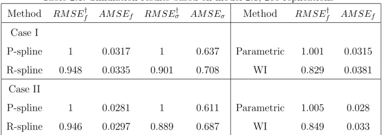
Table 2.1: Simulation results based on model 2.1, 200 replications Method RM SEf† AM SEf RM SE † σ AM SEσ Method RM SEf† AM SEf Case I P-spline 1 0.0317 1 0.637 Parametric 1.001 0.0315 R-spline 0.948 0.0335 0.901 0.708 WI 0.829 0.0381 Case II P-spline 1 0.0281 1 0.611 Parametric 1.005 0.028 R-spline 0.946 0.0297 0.889 0.687 WI 0.849 0.033
†RMSE: The ratio of AMSE between the proposed method and other methods.
In the second simulation model, we used f(t) = 7−16t+ 30t2−15t3 and σ2(t) =
10√t and all the other settings were the same as the first case.
We conducted 200 simulation runs. To evaluate performance of the estimated nonparametric functions, the mean squared errors (MSEs) were calculated over grid points {0.05,0.06,· · ·,0.95} for each simulated dataset. The MSEs were then aver-aged across the 200 simulated datasets to obtain the average MSE (AMSE). Table 2.1 summarizes the simulation results. The AMSEf and AMSEσ are the corresponding AMSEs of f(t) and σ2(t). The RMSEf and RMSEσ are the ratios of AMSE of the proposed P-spline estimators fb(t) and
b
σ2(t) over other estimators. The RMSE
f of the proposed method over assuming working independent residuals was around 0.85 for both simulation models which suggests efficiency gain of estimating mean function by properly accounting for the within-subject covariance by the proposed semipara-metric estimator. The RMSEf of the proposed P-spline estimator over the regression spline was about 0.95. The corresponding AMSEσ for the variance function of the proposed over the regression spline was about 0.90 for both simulation models, which shows the proposed method to be also more efficient (10% reduction in AMSE) in es-timating the variance function. To compare with the parametric approach assuming the functional form of the variance function to be known, we note that the RMSEf of the proposed over the parametric approach was slightly over one indicating low
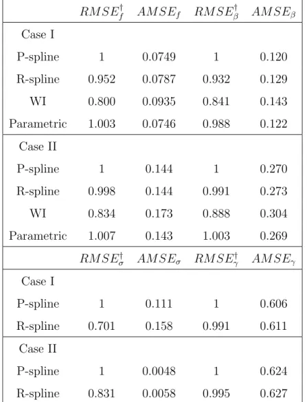
ef-Table 2.2: Simulation results based on model 2.5, 200 replications RM SEf† AM SEf RM SE † β AM SEβ Case I P-spline 1 0.0749 1 0.120 R-spline 0.952 0.0787 0.932 0.129 WI 0.800 0.0935 0.841 0.143 Parametric 1.003 0.0746 0.988 0.122 Case II P-spline 1 0.144 1 0.270 R-spline 0.998 0.144 0.991 0.273 WI 0.834 0.173 0.888 0.304 Parametric 1.007 0.143 1.003 0.269 RM SEσ† AM SEσ RM SEγ† AM SEγ Case I P-spline 1 0.111 1 0.606 R-spline 0.701 0.158 0.991 0.611 Case II P-spline 1 0.0048 1 0.624 R-spline 0.831 0.0058 0.995 0.627
†RMSE: The ratio of AMSE between the proposed method and other methods.
ficiency loss in adopting the proposed semiparametric approach to estimate variance functions.
Simulation Study II.
Our second simulation study examines methods proposed for the functional mixed effects model with varying coefficients and nonparametric random subject-specific curves in Section 2.3. We generated data from the model
where we considered two simulation scenarios. In the first scenario, we specified f(t) = 2 sin(2πt), β(t) = 1
3logt, ν(t) = 1.5 exp{−10(t−0.8)
2}, σ2(t) = exp(t).
The random coefficients bi0 and bi1 were sampled from N(0,4) and N(0,1),
respec-tively. The measurement errorsij(Tij) were generated independently fromN(0, σ2(Tij)). The group indicators, trti, were generated from Bernoulli distribution with probabil-ity 0.6. The total number of subjectsn = 200 while the repeated measurements within each subject m = 10 with probability 0.15 of being missing. The measurement time points were generated from U(0,1).
In the second scenario, we specified
f(t) = 2 exp{sin(4t)}, β(t) =√t, ν(t) = 0.7 exp(t), σ2(t) = exp{−5(t−0.1)2}, n = 100, and m= 20 with a missing probability of 0.15. All the other settings were the same as the first case.
The simulation results are summarized in Table 2.2. Again the AMSEf, AMSEβ, AMSEσ and AMSEγ are the corresponding AMSEs of f(t),β(t),σ2(t) andγ(t, t), re-spectively. The RMSEs are the ratios of the AMSE of the proposed method over other methods. Similar to the first simulation study, we compared the proposed estimators to regression spline (R-spline), P-spline assuming working independent residuals (WI) and P-spline assuming a correctly specified parametric model for the subject-specific random effects covariance and residual effects variance (Parametric). The efficiency gains of the proposed method for estimating the mean and varying coefficient function were about 15% compared to assuming working independent residuals in both simula-tion scenarios, which is non-ignorable. For estimating the mean funcsimula-tion, in the first scenario, the proposed method performed better than the regression spline in terms of AMSE, while in the second scenario their performance was similar. The AMESσ for estimating the covariance function was 30% lower for the P-spline compared to regression spline in the first scenario and 17% lower in the second scenario. Analogous to the simulation study I, the differences in AMSE between the parametric approach