A Family of Joint Sparse PCA Algorithms for Anomaly Localization in Network Data Streams

(1)

A Family of Joint Sparse PCA Algorithms for

Anomaly Localization in Network Data Streams

By

Ruoyi Jiang

Submitted to the graduate degree program in Department of Electrical Engineering and Computer Science and the Graduate Faculty of the University of Kansas in partial

fulﬁllment of the requirements for the degree of Master of Science

Committee members

Jun Huan, Chairperson

Victor Frost

Bo Luo

(2)

The Master Thesis Committee for Ruoyi Jiang certiﬁes that this is the approved version of the following master thesis :

A Family of Joint Sparse PCA Algorithms for Anomaly Localization in Network Data Streams

Jun Huan, Chairperson

(3)

Abstract

Determining anomalies in data streams that are collected and transformed from various types of networks has recently attracted significant research interest. Principal Component Analysis (PCA) is arguably the most widely applied un-supervised anomaly detection technique for networked data streams due to its simplicity and efficiency. However, none of existing PCA based approaches ad-dresses the problem of identifying the sources that contribute most to the ob-served anomaly, or anomaly localization. In this paper, we first proposed a novel joint sparse PCA method to perform anomaly detection and localization for network data streams. Our key observation is that we can detect anoma-lies and localize anomalous sources by identifying a low dimensional abnormal subspace that captures the abnormal behavior of data. To better capture the sources of anomalies, we incorporated the structure of the network stream data in our anomaly localization framework. Also, an extended version of PCA, multi-dimensional KLE, was introduced to stabilize the localization performance. We performed comprehensive experimental studies on four real-world data sets from different application domains and compared our proposed techniques with sev-eral state-of-the-arts. Our experimental studies demonstrate the utility of the proposed methods.

(4)

List of Figures

3.1 Illustration of time-evolving stock indices data . . . 15 3.2 Comparing PCA and Sparse PCA. . . 15 4.1 Demonstration of JSPCA on three network data streams with one anomaly

(solid line) and two normal streams (dot lines). . . 17 4.2 Comparing diﬀerent anomaly localization methods. From left to right: PCA, sparse

PCA, JSPCA, and GJSPCA.. . . 19 4.3 Comparingjoint sparse PCA(JSPCA) andgraph joint sparse PCA (GJSPCA). 19 4.4 From left to right: PC space for JSKLE and GJSKLE, abnormal score for

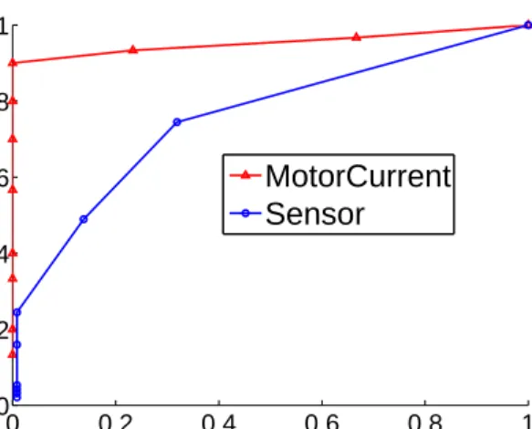
JSKLE, and GJSKLE. . . 22 5.1 ROC curve for anomaly detection on sensor dataset and motorCurrent dataset.

AUC for sensor dataset is 0.7832, for motorCurrent dataset is 0.9688 . . . . 41 5.2 ROC curves and AUC for diﬀerent methods on three data sets. From left to

right: ROC for the stock indices data, ROC for the sensor data, ROC curve for MotorCurrent data . . . 42 5.3 ROC curve for KLE extension methods on three data sets. From left to right:

ROC for the stock indices data, ROC for the sensor data, ROC curve for MotorCurrent data . . . 42 5.4 AUC for diﬀerent methods on three data sets . . . 43 5.5 pairwise ANOVA testing . . . 43

(7)

5.6 Anomaly Localization Performance of GJSPCA, Stochastic Nearest Neigh-borhood, Eigen-Equation Compression on Network Intrusion Data Set(DoS Attack) . . . 44 5.7 Most relevant features selected for diﬀerent attacks . . . 44 5.8 Left: original data in time interval [2001,3300] in sensor dataset. Right: time

series of abnormal score calculated from left ﬁgure (with window size 20 and oﬀset 10) . . . 45 5.9 Left: original data in time interval [7391,8000] in sensor dataset. Right: time

series of abnormal score calculated from left ﬁgure (with window size 20 and oﬀset 10) . . . 46 5.10 Left: original data in motorcurrent dataset. Right: time series of abnormal

score calculated from left ﬁgure (with window size 50 and oﬀset 25) . . . 46 5.11 Left: original data in time interval [341,420] on stock market dataset. Right:

time series of abnormal score calculated from left ﬁgure (with window size 20 and oﬀset 5) . . . 47 5.12 From left to right, sensitivity analysis of GSPCA on λ1,λ2, δ, and the dimension

of the normal subspace. . . 49 5.13 From left to right, sensitivity analysis of GJSKLE onλ1,λ2,δ, and the dimension

of the normal subspace. . . 50 5.14 Sensitivity analysis of GJSKLE on N. . . 50

(8)

List of Tables

3.1 Notations in the paper. . . 12 5.1 Characteristics of Data Sets. D: Data sets. D1: Stock Indices, D2: Sensor, D3:

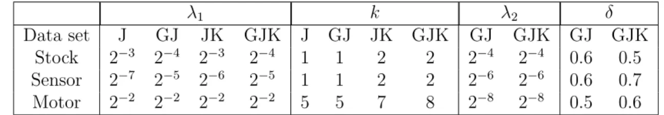
MotorCurrent, D4: Network Traﬃc. T: total number of time stamps, p: dimen-sionality of the network data streams, I: total number of intervals for anomaly localization,Indices: starting point and ending point of the intervals for anomaly localization, W: total number of data windows for anomaly localization, W2: to-tal number of data windows for anomaly detection L: sliding window size, -: not applicable. . . 35 5.2 Optimal parameters combinations on three data sets. J:JSPCA, GJ: GJSPCA,

JK:JSKLE, GJK: GJSKLE. The best temporal oﬀset is 2 for all data sets . . . . 40 5.3 Features Indexes in KDD 99 Intrusion Detection Data set . . . 45

(9)

Chapter 1 Introduction

Anomaly detection is an important problem that has been researched within diverse research areas and application domains. Anomaly detection refers to detecting the abnormal patterns in data that do not conform to established normal behavior. Those non-conforming patterns are referred to as outliers, change, deviation, surprise, aberrant, peculiarity, intrusion, etc. Over time, anomaly detection in data streams that are collected and transformed from various types of networks has recently attracted significant research interest in the data mining community [5, 24, 51, 59]. Applications of the work could be found in network traffic data [59], sensor network streams [5], social networks [51], cloud computing [44], and finance networks [24] among others. The importance of anomaly detection in network data stream is due to the fact that anomalies in network data stream is significant and critical information in a wide variety of application domains. For example, anomalous network traffic usually results from malicious activity such as break-ins and computer abuse which are interesting form a computer security perspective. An anomalous event in optical sensor network could mean that something is on fire. Anomalies in video surveillance may indicate insertion of foreign objects.

Besides anomaly detection, another outstanding data analysis issue is anomaly localiza-tion, where we aim to discover the speciﬁc sources that contribute most to the observed

(10)

anomalies. Anomaly localization in network data streams is apparently critical to many applications, including monitoring the state of buildings [58] to find the anomalous compo-nents, or locating the sites for flooding and forest fires [14]. In the stock market, pinpointing the change points in a set of stock price time series is also critical for making intelligent trad-ing decisions [37]. For network security, localiztrad-ing the sources of the most serious threats in computer networks helps quickly and accurately repair and ensure security in networks [32]. Principal Component Analysis (PCA) is arguably the most widely applied unsupervised anomaly detection technique for network data streams [21, 32, 33]. However, a fundamen-tal problem of PCA, as claimed in [48], is that the current PCA based anomaly detection methods can not be applied to anomaly localization. Our key observation is that the major obstacle for extending the PCA technique to anomaly localization lies in the high dimen-sionality of the abnormal space. If we manage to identify a low dimensional approximation of the high dimensional abnormal subspace using a few sources, we “localize” the abnormal sources. The starting point of our investigation hence is the recently studied sparse PCA framework [62] where PCA is formalized in a sparse regression problem where each principle component (PC) is a sparse linear combination of the original sources. However, sparse PCA does not fit directly into our problems in that sparse PCA enforces sparsity randomly in the normal and abnormal subspaces. In my thesis, we explore several directions in improving sparse PCA for anomaly detection and localization.

First, we develop a new regularization scheme to simultaneously calculate the normal subspace and the sparse abnormal subspace. In the normal subspace, we do not add any regularization but use the same normal subspace as ordinary PCA for anomaly detection. In the abnormal subspace, we enforce that diﬀerent PCs share the same sparse structure hence it is able to do anomaly localization. We call this methodjoint space PCA (JSPCA).

Second, we observe that abnormal streams are usually correlated to each other. For example in stock market, index changes in diﬀerent countries are often correlated. For incorporating stream correlation in anomaly localization we design a graph guided sparse

(11)

PCA (GJSPCA) technique. Our experimental studies demonstrate the eﬀectiveness of the proposed approaches on three real-world data sets from ﬁnancial markets, wireless sensor networks, and machinery operating condition studies.

Another drawback of PCA is it only considers the spatial correlation between different streams but ignores the temporal correlation between different time stamps [4]. In order to overcome this problem, we introduce a multi-dimensional Karhunen Loève Expansion (KLE) as an extension of PCA to take care of both temporal and spacial correlations. PCA is a special case of multi-dimensional KLE with only spacial dimension. The corresponding methods are called joint space KLE (JSKLE) and graph guided sparse KLE (GJSKLE) respectively. The experiments proves that the JSKLE and GJSKLE stabilizes localization performance effectively when considering both spatial and temporal correlations.

The remainder of the thesis is organized as follows. In chapter 2, we present related work of anomaly localization. In chapter 3, we discuss the challenge of applying PCA to anomaly localization. In chapter 4 we introduce the formulation of JSPCA and GJSPCA, and their extended version JSKLE, GJSKLE, and the related optimization algorithm. We present our experimental study in chapter 5 and conclude in chapter 6.

(12)

Chapter 2 Related Work

Anomaly detection and localization has been the topic of a number of articles and books. Next, I will ﬁrst introduced several techniques used in anomaly detection and anomaly localization. A variety of anomaly detection and localization techniques have been developed in several research communities, some are speciﬁcally for certain application domain, some are generic and applicable for many domain. Then we will cover the applications of these techniques. Anomaly detection and localization have extensive use in a wide variety of applications such as intrusion detection for computer security, fraud detection for credit cards, insurance or health care, fault detection in condition monitoring systems and so on.

2.1 Current Anomaly Detection Techniques

There are a variety of methodologies used to do anomaly detection. Here we focus on data mining-based anomaly detection techniques. Data mining techniques are well suited to anomaly detection problem because it is a process of extracting “patterns” from large volume of data. Speciﬁcally, when applied to network anomaly detection, data mining techniques construct models that could automatically discover the consistent and useful patterns of normal behaviors from the network data, and use these patterns to recognize anomalies and intrusions.

(13)

Based on whether data samples are labeled or not, the approaches fall into two categories: supervised anomaly detection and unsupervised anomaly detection. Supervised outlier de-tection techniques require the availability of a labeled training data set with labeled instances for the normal as well as the outlier class. In such techniques, predictive models are built for both normal and outlier classes. Any unseen data instance is compared against the two mod-els to determine which class it belongs to. There are two major issues in supervised learning algorithms. First, training data is imbalanced because the anomalous instances are far fewer compared to the normal instances. Second, obtaining accurate labels is usually challenging. Other than these two issues, the supervised anomaly detection problem is similar to building predictive models.

Most supervised anomaly detection algorithms are classification based. In the training phase, a classifier is learned using the available labeled training data. In the testing phase, a test instance is classified as normal or anomalous using the classifier. Popular classifiers include neural network, Bayesian network, Support Vector Machines and ruled based. A neural network is trained on the normal training data to learn the different normal classes and then each test instance is provided as an input to the neural network. If the network accepts the test input, it is normal and if the network rejects a test input, it is an anomaly [25, 40]. Bayesian networks have also been widely used. A basic technique using a naive Bayesian network estimates the posterior probability of observing a class label (from a set of normal class labels and the anomaly class label), given a test data instance. The class label with largest posterior is chosen as the predicted class for the given test instance [54, 55]. Support Vector Machines (SVMs) have been applied to anomaly detection in the one-class setting since 1995. Such techniques use one class learning techniques for SVM and learn a region that contains the training data instances (a boundary). If a test instance falls within the learnt region, it is declared as normal, else it is declared as anomalous [46, 60]. Rule based anomaly detection techniques learn rules that capture the normal behavior of a system. A test instance that is not covered by any such rule is considered as an anomaly [56, 50].

(14)

An unsupervised outlier detection technique makes no assumption about the availability of labeled training data. Thus, these techniques are more widely applicable. Several unsu-pervised techniques make the basic assumptions such that the majority of the instances in the data set are normal. Nearest neighbor based techniques, clustering, statistical model and spectrum anomaly detection are most popular unsupervised anomaly detection techniques. Nearest neighbor based techniques based on an assumption that normal data instances oc-cur in dense neighborhoods, while anomalies ococ-cur far from their closest neighbors. Basic nearest neighbor anomaly detection techniques can be broadly grouped into two categories: anomaly score is the distance of data instance to its kth nearest neighbor, or computed as the density of the data instance. Clustering based techniques usually consist of two steps. First, the data is clustered using a clustering algorithm such as k-means, Expectation Maxi-mization and DBSCAN. In the second step, for each data instance, its distance to its closest cluster centroid is calculated as its anomaly score [15, 35, 17]. Statistical techniques usually have some assumption on the distribution of given data. By applying statical inference test we determine if an unseen instance is normal or abnormal. Normal instances occur in high probability regions of the statistical model while anomalies occur in a low probability regions of the stochastic model [18, 52]. Spectral anomaly detection techniques try to find a lower dimensional subspace in which normal instances and anomalies appear significantly different. Principal Component Analysis is the most widely used. Principal Components capture the normal and abnormal behaviors underlying the data and projection of data instances on principal components is used to make detection decision [21].

From another point of view, based on the data used in detection procedure, anomaly detection from network data streams are divided into two categories: those at the source level and those at the network level. The source level anomaly detection approaches embed detection algorithm at each stream source, resulting in a fully distributed anomaly detection system [19, 34, 44]. Detection is based on individual data and decision is made for each source. The major problems of these approaches are two folds: some source level anomalies

(15)

may not be indicative of network level anomalies due to the ignorance of the rest of the network [21], and there may not be available space to perform anomaly detection in each source. To improve source level anomaly localization methods, several algorithms have been recently proposed to anomaly at the network level. The network level anomaly detection approaches take the whole network into consideration. Since the decision is made based on the entire network, the network level anomaly detection approaches are not as knowledgeable about any source speciﬁcs. This leads to one of the major restrictions: they usually fail to pinpoint which sources should be responsible for the anomalies, that is, anomaly localization.

2.2 Current Anomaly Localization Techniques

Source level anomaly detection embeds detection algorithm at each stream source and makes decision for each source. Hence anomaly detection and anomaly localization are ﬁnished in one step. For network level anomaly detection, anomaly localization is an additional step after anomaly detection. More speciﬁcally, network level anomaly detection is a binary decision such that whether the whole network is normal or abnormal. If the network is abnormal, we need to go one step further to determine which sources are responsible for the observed anomaly.

Some algorithms have been recently proposed to localize anomaly at the network level. Brauckhoff [3] applied association rule mining to network traffic data to extract abnormal flows from the large set of candidate flows. Their work is based on the assumption that anomalies often result in many flows with similar characteristics. Such an assumption holds in network traffic data streams but may not be true in other data streams such as finance data. Keogh et al.[30] proposed a nearest neighbor based approach to identify abnormal subsequences within univariate time series data by sliding windows. They extracted all possible subsequences and located the one with the largest Euclidean distance from its closest non-overlapping subsequences. However, the method only works for univariate time series

(16)

generated from a single source. In addition, if the data is distributed on a non-Euclidean manifold, two subsequences may appear deceptively close as measured by their Euclidean distance [53]. L. Fonget al.developed a nonparametric change-point test based on U-statistics to detect and localize change-points in high-dimensional network traﬃc data [38]. The limitation is that the method is speciﬁcally designed for the Denial of Service (DOS) attack in communication networks and cannot be generalized to other types of network data streams easily.

Most related to our work, Ide et al.[22, 23] measured the change of neighborhood graph for each source to perform anomaly localization and developed a method called Stochastic Nearest Neighbor (SNN). Hirose et al.[20] designed an algorithm named Eigen Equation Compression (EEC) to localize anomalies by measuring the deviation of covariance matrix of neighborhood sources. In these two studies, we have to build a neighborhood graph for each source for each time interval, which is unlikely to scale to a large number of sources. In [28], we proposed a two step approach that ﬁrst computed normal subspace from ordinary PCA and then derived a sparse abnormal subspace on the residual data subtracted from the original data.

2.3 Applications of Anomaly Detection and Anomaly

Localization

Applications of anomaly detection could be found in computer related system [59], sensor network streams [5], social networks [51], cloud computing [44], and ﬁnance networks [24] among others.

Detection of malicious activity in computer related system refers to intrusion detection. The malicious activities include ﬂood-type attack, break-ins, and other forms of computer abuse. These attacks are diﬀerent from the normal behavior of the computer system, and hence anomaly detection techniques are applicable in intrusion detection domain. There

(17)

are multiple data sources for intrusion detection and the common ones are at host level and network level. Based on the sources, Intrusion Detection System (IDS) are grouped into Host-Based IDS and Network-Based IDS. These intrusion detection systems were responsible for the security of an individual (host) machine instead of the security of the network as a whole. In contrast to a host-based IDS, a network-based IDS monitors and protects the network as a whole. The key challenge for intrusion detection is the large volume of data. Such data usually involves thousands of connections so the anomaly detection techniques need to be computationally eﬃcient to handle these large sized inputs.

Fraud detection is another anomaly detection application which is applicable to many industries including banking and ﬁnancial sectors, insurance, credit card companies, stock market and more [47, 45]. The fraud cases have to be detected from the available huge data sets such as the logged data and user behaviors. The types of frauds mostly discussed in recent papers are credit card frauds, mobile phone frauds, and insurance claim fraud. The most important requirement of anomaly detection techniques in this domain is to detect fraud in an online manner and as early as possible.

Anomaly detection and localization involving image data are are either interested in motion detection and localization (changes in an image over time) or in abnormal regions detection and localization on the static image [39, 6]. Image data has spatial as well as temporal characteristics, hence anomaly analysis has to be done in both spatial and temporal domain. One of the key challenges in this domain is the large size of the input. When dealing with video data, online techniques are required.

When applied to sensor network, anomaly detection and localization are usually respon-sible to detect faulty sensor from sensor network or detect events that are interesting for analysis. For instance, anomaly detection is a critical step in nature disaster monitoring including flooding and forest fire monitoring. Due to severe sensor resource constraints, the anomaly detection and localization techniques need to be power efficient. Another challenge is data is collected in a distributed fashion, and hence a distributed data mining approach

(18)

is required to analyze the data [7, 57].

Anomaly detection has also been applied to several other domains such as detecting novel topics or events a collection of documents or news articles, detecting anomalies in biological data, detecting users whose behavior deviates from the usual behavior in a social network.

(19)

Chapter 3 Preliminaries

We introduce the notations used in this paper and background information regarding PCA and sparse PCA.

3.1 Notation

We use uppercase calligraphic letters such asXto denote a matrix and bold lowercase letters such asxto denote a vector. Greek letters such asλ1, λ2 are Lagrangian multipliers. ⟨A,B⟩

represents the matrix inner product deﬁned as ⟨A,B⟩=tr(ATB) where tr represents the matrix trace. Given a matrix X we use xij to denote the entry of X at the ith row and jth column. We use xi to represent the ith entry of a vector x. ||x||p = (

∑n i=1|xi|

p₎p1 denotes the lp norm of the vector x ∈ Rn. Given a matrix X ∈ Rn×p, ∥X∥1,q =

∑n

i=1∥˜xi∥q is the

l1/lq norm of the matrix X, where ˜xi is the ith row of X in column vector form. Unless stated otherwise, all vectors are column vectors. In Table 3.1, we summarize the notations in our paper.

(20)

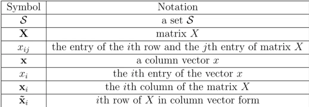
Table 3.1: Notations in the paper.

Symbol Notation

S a set S

X matrix X

xij the entry of the ith row and thejth entry of matrixX

x a column vectorx

xi the ith entry of the vector x xi the ith column of the matrix X ˜

xi ith row of X in column vector form

3.2 Network Data Streams

Our work focuses on data streams that are collected from multiple sources. We call the set of data stream sources together as a network since we often have information regarding the structure of the sources.

Following [10], Network Data Streams are multi-variate time series S from p sources where S ={Si(t)} and i∈[1, p]. p is the dimensionality of the network data streams. Each function Si : R → R is a source. A source is also called a “node” in the communication network community and a “feature” in the data mining and machine learning community.

Typically we focus on time series sampled at (synchronized) discrete time stamps{t1, t2, . . . , tn}. In such cases, the network data streams are represented as a matrix X = (xi,j) where i∈[1, n], j ∈[1, p] and xi,j is the reading of the stream source j at the time sample ti.

3.3 Applying PCA for Anomaly Localization

Our goal is to explore a Principal Component Analysis (PCA) based method for performing anomaly detection and localization simultaneously. PCA based anomaly detection technique has been widely investigated in [32, 21, 33]. In applying PCA to anomaly detection, one ﬁrst constructs the normal subspace V1 _{by the top} _k _{PCs and the abnormal subspace}_V2 _{by the}

remaining PCs, then projects the original data on V(1) _and _V(2) _as:

(21)

whereX∈ Rn×p _{is the data matrix with}_n _{time stamps from} _p_{data sources,}_X

n and Xa are the projections ofXon normal subspace and abnormal subspace respectively. The underlying assumption of PCA based anomaly detection is thatXncorresponds to the regular trends and Xa captures the abnormal behaviors in the data streams. By performing statistical testing on the squared prediction error SP E = tr(XT

aXa), one determines whether an anomaly happens [21, 32]. The larger SP E is, the more likely an anomaly exists.

Although PCA has been widely studied for anomaly detection, it is not applicable for anomaly localization. The fundamental problem, as claimed in [48], lies in the fact that there is no direct mapping between two subspaces V(1), V(2) and the data sources. Speciﬁcally,

let V(2) = [vk+1,· · · ,vp] be the abnormal subspace spanned by the last p−k PCs, Xa is essentially an aggregated operation that performs linear combination of all the data sources, as follows: Xa =XV(2)V₍₂₎T = [ _p ∑ j=1 xjv˜Tj˜v1,· · · , p ∑ j=1 xj˜vTjv˜i,· · · , p ∑ j=1 xj˜vjT˜vp−k ] (3.2)

wherexj is the data from thejth source and˜vj is thejth row ofV2 in column vector form.

Considering the ith column of Xa with the value

∑p

j=1xjv˜j˜v

T

i , there is no correspondence between the originalith column ofXandith column ofXa. Such an aggregation makes PCA diﬃcult to identify the particular sources that are responsible for the observed anomalies.

Although all the previous works claim PCA based anomaly detection methods cannot

do localization, we solve the problem of anomaly localization in a reverse way. Instead of locating the anomalies directly, we ﬁlter normal sources to identify anomalies by employing the fact that normal subspace captures the general trend of data and normal sources have little or no projection on abnormal subspace. The following provides a necessary condition for data sources to have no projection on abnormal subspace.

Suppose I = {i|˜vi = 0} is the set that contains all the indices for the zero rows of V(2), then ∀t ∈ S, xt has no projection on the abnormal subspace. In other words, these sources have no contribution to the abnormal behavior. Consider the squared prediction

(22)

error SP E =tr(XT

aXa) and plug equation 3.2 in: tr(XT aXa) = tr(XaXTa) = tr(VT 2XTXV2) = tr((∑p_j₌₁xj˜vjT)T( ∑p j=1xj˜vTj)) = p ∑ i=1 p ∑ j=1 tr(˜vixTi xjv˜Tj) = ∑ i /∈I ∑ j /∈I (xT_ixj˜vjT˜vi). (3.3)

From equation (3.3), it is clear that ∀i∈ I, the data xi from sourcei has no projection on abnormal subspace and hence would be excluded from the statistics used for anomaly detection. We call such a pattern with an entire row with zeros “joint sparsity”.

Unfortunately ordinary PCA does not guarantee any sparsity in PCs. Sparse PCA is a recently developed algorithms where each PC is a sparse linear combination of the original sources [62]. However existing sparse PCA method has no guarantee that diﬀerent PCs share the same sparse representation and hence has no guarantee for the joint sparsity.

To illustrate the point, we show the following example of anomaly detection and anomaly localization in network data streams. This example will be used in the following chapters as well.

We plot the normalized stock index streams of eight countries over a period of three months in Figure 3.1. We notice an anomaly in the marked window between time stamps 25 and 42. In that window sources 1, 4, 5, 6, 8 (denoted by dotted lines) are normal sources. Sources 2, 3, 7 (denoted by solid lines) are abnormal ones since they have a diﬀerent trend from that of the other sources. In the marked window, the three abnormal sources clearly share the same increasing trend while the rest share a decreasing trend.

we plotted the entries of each PC for ordinary PCA and for sparse PCA (ﬁgure 3.2) for the stock data set shown in ﬁgure 3.1. White blocks indicate zero entries and the darker color indicates a larger absolute loading. Sparse PCA produces sparse entries but that alone

(23)

0 10 20 30 40 50 60 70 −0.2 0 0.2 0.4 0.6 0.8 1 1.2 T source1 source 2 source 3 source 4 source 5 source 6 source 7 source 8

Figure 3.1: Illustration of time-evolving stock indices data does not indicate sources that contribute most to the observed anomaly.

Below we present our extensions of PCA that enable us to reduce dimensionality in the abnormal subspace.

Sources

PCs

PCA 2 4 6 8 2 4 6 8 Sources PCs SPCA 2 4 6 8 2 4 6 8

(24)

Chapter 4 Sparse PCA for Anomaly Localization

In this section, we propose a novel regularization framework called joint sparse PCA (JSPCA) to enforce joint sparsity in PCs in the abnormal space while preserving the PCs in the normal subspace so that we can perform simultaneous anomaly detection and anomaly localization. Then we consider the network topology in the original data and incorporate such topology into JSPCA and develop an approach named Graph JSPCA (GJSPCA). We also extend JSPCA and GJSPCA to JSKLE and GJSKLE, which taking the temporal correlation into account as well as spatial correlation considered in JSPCA and GJSPCA.

4.1 Joint Sparse PCA

Our objective here is to derive a set of PCs V = [V(1)_,_V(3)_{] such that} _V(1) _{is the normal}

subspace andV(3)_{is a sparse approximation of the abnormal subspace with the joint sparsity.}

The following regularization framework guarantees the two properties simultaneously:

min V(1)_,V(3) 1 2||X−XV (1)_V(1)T ₋_XV(3)_V(3)T_||2 F +λ||V(3)||1,2 s.t. VT_V ₌_I p×p. (4.1)

(25)

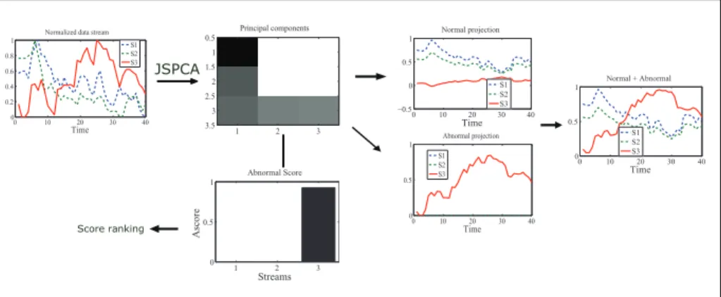
Score ranking 0 10 20 30 40 0 0.2 0.4 0.6 0.8 1

Normalized data stream

Time S1 S2 S3 Principal components 1 2 3 0.5 1 1.5 2 2.5 3 3.5 0 10 20 30 40 −0.5 0 0.5 1 Normal projection Time S1 S2 S3 0 10 20 30 40 0 0.5 1 Abnormal projection Time S1 S2 S3 0 10 20 30 40 0 0.5 1 Normal + Abnormal Time S1 S2 S3 1 2 3 0 0.5 1 Abnormal Score A sc or e Streams JSPCA

Figure 4.1: Demonstration of JSPCA on three network data streams with one anomaly (solid line) and two normal streams (dot lines).

Using one variableV, we simplify equation (4.1) as:

min V 1 2||X−XVV T_||2 F +λ||W◦V||1,2 s.t. VT_V ₌_I p×p. (4.2)

Here◦ is the Hadamard product operator (entry-wise product), λ is a scalar controlling the balance between sparse and ﬁtness, W = [w˜1,· · · ,w˜p]T with w˜j is deﬁned below:

˜ wj = [0_{| {z }},· · · ,0 k ,1_{| {z }},· · · ,1 p−k ]T, j = 1,· · · , p. (4.3)

The regularization term∥W◦V∥1,2 is aL1/L2 penalty which enforces joint sparsity for each

source across in the abnormal subspace spanned by the remainingp−kprincipal components.

The major disadvantage of equation (4.2) is that it poses a diﬃcult optimization problem since the ﬁrst term (the trace norm) is concave and the second term (theL1/L2 norm) is

con-vex. The similar situation was first investigated in sparse PCA [62] with elastic net penalty [61], in which two variables and an alternative optimization algorithm were introduced. Here we share the first least square loss term but with a different regularization term. Motivated

(26)

by [62], we consider a relaxed version: min A,B 1 2||X−XBA T_||2 F +λ||W◦B||1,2 s.t. ATA =Ip×p, (4.4)

Where A,B ∈ Rp×p_{. The advantage of the new formalization is two folds: first, equation} (4.4) is convex to each subproblem when fixing one variable and optimizing the other. As asserted in [62] disregarding the Lasso penalty, the solution of equation (4.4) corresponds to exact PCA; second, we only impose penalty on the remaining p−k PCs and preserve the top k PCs representing the normal subspace from ordinary PCA. Such a formalization will guarantee that we have the ordinary normal subspace for anomaly detection and the sparse abnormal subspace for anomaly localization. Note that Jenatton et al.recently proposed a structured sparse PCA [26], which is similar to our formalization. But their structure is defined on groups and cannot be directly applied for anomaly localization.

Figure 4.3 demonstrates the principal components generated from JSPCA for the stock market data shown in figure 3.1. Joint sparsity across the PCs in abnormal subspace pin-points the abnormal sources 2,3,7 by filtering out normal sources 1, 4, 5, 6, 8. Such result matches the truth in figure 3.1.

4.2 Anomaly Scoring

To quantitatively measure the degree of anomalies for each source, we deﬁne anomaly score and normalized anomaly score as following.

Definition 4.2.1 Given p sources and the abnormal subspace V(3) _{= [}_v

k+1,· · · ,vp] from

(27)

1 2 3 4 5 6 7 8 0 0.5 1

Ascore

Sources

PCA 1 2 3 4 5 6 7 8 0 0.5 1

Ascore

Sources

SPCA 1 2 3 4 5 6 7 8 0 0.5 1

Ascore

Sources

JSPCA 1 2 3 4 5 6 7 8 0 0.5 1

Ascore

Sources

GJSPCA

Figure 4.2: Comparing diﬀerent anomaly localization methods. From left to right: PCA, sparse PCA, JSPCA, and GJSPCA.

Sources PCs JSPCA 2 4 6 8 2 4 6 8 Sources PCs GJSPCA 2 4 6 8 2 4 6 8

Figure 4.3: Comparing joint sparse PCA(JSPCA) and graph joint sparse PCA (GJSPCA).

of V(3)_{, divided by the size of the row:}

ζ = p ∑ j=k+1 |v˜ij| , (4.5)

(28)

where v˜ij is the ith entry of vj.

For each input data matrix X, (4.5) results in a vector ζ = [ζ1,· · · , ζp]T of anomaly

scores. The normalized score for source i is defined as:

˜

ζi =ζi/max{ζi, i= 1,· · ·p}.

A higher score indicates a higher probability that a source is abnormal. We show the anomaly scores obtained from PCA, SPCA, JSPCA, for the stock data in Figure 4.2. JSPCA succeeds to localize three anomalies by assigning nonzero scores to anomalous sources and zero to normal ones, while PCA and SPCA both fail. With abnormal scores, we can rank abnormality or generate ROC curve to evaluate localization performance. Bellow, we give a skeleton of algorithm for computing abnormal score and the detailed optimization algorithm is introduced later.

Algorithm 1 Anomaly Localization with JSPCA

1: Input: X, k and λ1.

2: Output: anomaly scores.

3: Calculate a set of PCs V = [V(1)_,_V(3)_{] (matrix} _B _{in equation (4.4)),} _V(1) _{is normal}

subspace, V(3) _{is abnormal subspace with joint sparsity;}

4: Compute abnormal score for each source by the deﬁnition (4.2.1);

4.3 Graph Guided Joint Sparse PCA

In many real-world applications, the sources generating the data streams may have structure, which may or may not change with time. As the example mentioned in ﬁgure 3.1, stock indices from source 2, 3 and 7 are closely correlated over a long time interval. If source 2 and 3 are anomalies as demonstrated in Figure 4.3, it is very likely that source 7 is an anomaly as well. This observation motivates us to develop a regularization framework that enforce smoothness across features. In particular, we model the structure among sources with an undirected graph, where each node represents a source and each edge encodes a possible

(29)

structure relationship. We hypothesize that incorporating structure information of sources we can build a more accurate and reliable anomaly localization model. Below, we introduce the graph guided joint sparse PCA, which eﬀectively encodes the structure information in the anomaly localization framework.

To achieve the goal of smoothness of features, we add an extended l2 (Tikhonov)

regu-larization factor on the graph laplacian regularized matrix norm of thep−kPCs. This is an extension of thel2 norm regularized Laplacian on a single vector in [12]. With this addition,

we obtain the following optimization problem:

min A,B 1 2||X−XBA T_||2 F +λ1∥W◦B∥1,2+ 1 2λ2tr((W◦B) T_L₍_W_◦_B₎₎ s.t. AT_A₌_I p×p, (4.6) ,

where L is the Laplacian of a graph that captures the correlation structure of sources [12].

In Figure 4.3 we show the comparison of applying JSPCA and GJSPCA on the data shown in ﬁgure 3.1. Both JSPCA and GJSPCA correctly localize the abnormal sources 2,3,7. Comparing JSPCA and GJSPCA, we observe that in GJSPCA the entry values corresponding to the three abnormal sources 2,3,7 are closer (a.k.a. smoothness in the feature space). In the raw data, we observe that sources 2,3,7 share an increasing trend. The smoothness is the reﬂection of the shared trend and helps highlight the abnormal source 7. As evaluated in our experimental study, GJSPCA outperforms JSPCA. We believe that the additional structure information utilized in GJSPCA helps.

The same observation is also shown in Figure 4.2. Comparing JSPCA and GJSPCA we find that JSPCA assigns higher anomaly scores to source 2 and 3 but a lower score to source 7, and GJSPCA has smooth effect on the abnormal scores. It assigns similar scores for the three sources. The similar scores demonstrate the effect of smooth regularization

(30)

Sources

PCs

JSKLE 2 4 6 8 2 4 6 8

Sources

PCs

GJSKLE 2 4 6 8 2 4 6 8 1 2 3 4 5 6 7 8 0 0.5 1

Ascore

Sources

JSKLE 1 2 3 4 5 6 7 8 0 0.5 1

Ascore

Sources

GJSKLE

Figure 4.4: From left to right: PC space for JSKLE and GJSKLE, abnormal score for JSKLE, and GJSKLE.

term induced by the graph Laplacian. The smoothness also sheds light on the reason why GJSPCA outperforms JSPCA a little in anomaly localization in our detailed experimental evaluation.

4.4 Extension with Karhunen Lo`

eve Expansion

In this section, we extend our previous work with multi-dimensional discrete KLE. KLE was ﬁrst considered as a representation of a stochastic process on an inﬁnite linear combination of orthogonal functions [16], and usually named as continuous KLE. Later on, discrete KLE was then given [31] and the its one dimensional version (PCA) has been successfully applied to a broad domain of applications [32, 11]. The advantage of KLE over PCA is that KLE

(31)

takes both spatial and temporal correlation into consideration while PCA only considers the spatial correlation.

In [4], Brauckhoﬀ et al. claimed that by extending PCA to KLE, they stabilized the anomaly detection performance and solved the sensitivity problem of PCA when changing the number of principal components representing the normal subspace [48]. Since JSPCA and GJSPCA are based on PCA, they both involve the same problem proposed in [48]. Therefore, we extend our regularization framework to KLE, called JSKLE and GJSKLE respectively towards the goal of stabilizing localization performance, which is illustrated in our experimental studies.

Generalize PCA to KLE amounts for expanding the original data matrix X ∈ Rn×p _to X′ ∈ R(n−N+1)×pN _{in both spatial and temporal domain as follows:}

X′T =                      x1(1) · · · x1(t) · · · x1(n−N+ 1) . . . . .. ... . .. ... x1(N) · · · x1(t+N−1) · · · x1(n) . . . . .. ... . .. ... xp(1) · · · xp(t) · · · xp(n−N+ 1) . . . . .. ... . .. ... xp(N) · · · xp(t+N−1) · · · xp(n)                      (4.7)

where N is the oﬀset moving forward in temporal domain.

Our staring point is a one dimensional stochastic process x(t) with zero mean over time intervalt ∈[a, b]. By the deﬁnition of KLE, x(t) admits a decomposition [49]:

x(t) =

∞

∑

i=1

αiψi(t) (4.8)

(32)

orthogonal deterministic functions such that ˆ D ψi(t)ψj(t)dt =δij δij =      0 if i̸=j 1 if i=j (4.9)

SupposeKx(t, s) is the continuous covariance function ofx(t), s.t.: Kx(t, s) =E[X(t)X(s)), ψi are eigenfunctions of Kx(., .) and derived by solving the Fredholm integral equation:

ˆ b

a

Kx(t, s)ψj(s)ds=λiψi(t) (4.10)

The uncorrelated random coeﬃcients αi are calculated as αi =

´b

a x(t)ψi(t)dt.

In real world applications, we can only access to discrete and ﬁnite processes. When applying to a discrete and ﬁnite process, KLE discretizes the parameter t to obtain the discrete version on temporal domain. Suppose a continuous stochastic processx(t) is sampled at an equal interval △t and an dimension vector xis

x= [x(1), x(2). . . x(n)]T (4.11)

wheren = b_△−_ta. In discrete version, covariance functionKx(t, s) turns into covariance matrix:

Γxx =E(xxT) (4.12)

To estimate the covariance matrix Γxx, we use sliding window averaging algorithm as the covariance estimator [41]. In this algorithm, computation of the estimated covariance matrix essentially involves the averaging of outer products of a sliding window over x. More specif-ically, a window of ﬁxed size N moves forward in x. Each time it forms a N-dimensional vector and the outer product is calculated. Averaging those outer products over all the

(33)

vectors yields the estimated covariance matrix.

Definition 4.4.1 Given a scaler time series x, the estimate of covariance matrixΓxx using

a sliding window approach is defined as:

Γxx = n−∑N+1

i=1

xixiT (4.13)

wherexi = [xi, xi+1, . . . , xi+N−1]T is the subvector of vectorxwith lengthN. A normalization

factor is ignored, since it is irrelevant for the eigenvectors of Γxx.

The summation function in (4.13) can be given in matrix format Γxx = XTX, with the following expanded data matrix X from a single vectorx in (4.11):

XT =          x(1) x(2) . . . x(n−N + 1) x(2) x(3) . . . x(n−N + 2) .. . ... . .. ... x(N) x(N+ 1) . . . x(n)          (4.14)

The integral equation (4.10) becomes a matrix eigenvector problem to solve the KLE vector (or principal component) associated with X: Γxxψi =λiψi

The eigenvectors ψi capture the temporal correlation of one discrete stochastic process (one stream) while the ordinary PCA we refereed previously, considers the spatial correlation among diﬀerent streams. In order to take both temporal and spatial correlation into account, we extended KLE from one dimension to multi-dimensions to deal with multiple stochastic processes.

From [49], ap-dimensional stochastic process frompsources is deﬁned: X = [xT

1,xT2,· · ·xTp]T. The ith component xi from the ith source takes the form in (4.11). Followed the equation (4.12), covariance matrix is deﬁned as:

(34)

with the following covariance structure: ΓXX =       Γx1x1 · · · Γx1xp .. . . .. ... Γxpx1 · · · Γxpxp      

Consider the covariance matrix estimator for one dimension KLE in equation (4.14) and its corresponding data matrix format in (4.14), we have the data matrix X′ for multi-dimensional KLE deﬁned in (4.7). The corresponding eigen vectors, which can be found by solving ΓXXψi =λiψi considering both the temporal and spatial correlation.

However, it is nontrivial to adopt the regularization framework proposed in (4.4) and (4.6) to expanded data matrix X′ because the data stream from each source has been extended from a vector to a matrix. The model parameters corresponding to each source also become a matrix, namelyB = [BT

1, B2T,· · ·, BpT]T where Bi is aN bypN matrix. The top k PCs ofB representing the normal subspace in regular PCA will becomekN PCs after KLE extension. Similarly, abnormal subspace is the rest (p−k)N PCs of B. More speciﬁcally, we consider the following optimization problem similar to the objective of JSKLE:

min A,B 1 2||X ′₋_X′_BAT_||2 F +λ1 p ∑ j=1 ||Wj ◦Bj||F s.t. ATA =IpN×pN, (4.16)

whereWj ∈ {0,1}N×pN is the jth matrix block ofWT = [W1,W2,· · · ,Wp] similar to (4.3) with ﬁrst kN columns being 0s and the rest being 1s:

Wj =       0 · · · 0 1 · · · 1 .. . . .. ... ... ... ... 0 · · · 0 1 · · · 1      

(35)

ex-tended data. Since each source has been exex-tended to multiple streams, we take average values across theN extended streams and make the average values smooth according to the network topology. More formally, considering the following objective:

min A,B 1 2||X ′₋_X′_BAT_||2 F +λ1 p ∑ j=1 ||Wj ◦Bj||F 1 2Nλ2tr((W◦B) T_PT_LP₍_W◦_B₎₎ s.t. ATA =IpN×pN, (4.17)

where P∈ {0,1}p×pN _{is used to summing each block of} _B _{and deﬁned as:}

P=          1 · · · 1 0 · · · 0 · · · 0 · · · 0 0 · · · 0 1 · · · 1 · · · 0 · · · 0 .. . . .. ... ... ... ... ... ... ... ... 0 · · · 0 0 · · · 0 · · · 1 · · · 1         

In Figure 4.4, we show the PC space computed from JSKLE and GJSKLE. There are two principal components representing the normal subspace and the rests presenting the ab-normal subspace. Both JSKLE and GJSKLE highlight the abab-normal sources while GJSKLE shows a smooth eﬀect on 3 abnormal sources 2, 3, 7.

For JSKLE and GJSKLE, the deﬁnition of abnormal score is a little diﬀerent from that of JSPCA and GJSPCA. Suppose the abnormal subspace is given byV(3)T

= [V(3)

1,V(3)2,· · · ,V(3)p] (the rest (p − k)N columns of B from (4.16) or (4.17)), the anomaly score for source i, i= 1· · ·pis

ζi =

||V(3)_i ||1

(p−k)N (4.18)

where V(3)_i is the ith matrix block of V(3)_.

Abnormal scores computed by JSKLE and GJSKLE are shown in Figure 4.4. JSKLE and GJSKLE performs similarly to JSPCA and GJSPCA but they are insensitive to the number of PCs representing the normal subspace, which will be studied in our experimental

(36)

studies.

4.5 Optimization Algorithms

We present our optimization technique to solve equations (4.4), (4.6), (4.16) and (4.17) based on accelerated gradient descent [43] and projected gradient scheme [2]. Since (4.16) and (4.17) are similar to (4.4) and (4.6), our following discussion will focus on (4.4) and (4.6). The solutions for (4.16) and (4.17) can be obtained by the same procedure with only minor changes on calculating gradient and gradient projection.

Although equations (4.4) and (4.6) are not joint convex for Aand B, they are convex for A and B individually. The algorithm solvesA, B iteratively and achieves a local optimum. A given B: IfB is ﬁxed, we obtain the optimalA analytically. Ignoring the regulariza-tion part, equaregulariza-tion (4.4) and equaregulariza-tion (4.6) degenerate to

min A 1 2||X−XBA T_||2 F s.t. AT_A ₌_I p×p. (4.19)

The solution is obtained by a reduced rank form of the Procrustes Rotation. We compute the SVD ofGB to obtain the solution where G=XTX is the gram matrix:

GB = UDVT ˆ

A = UVT_.

(4.20)

Solution in the form of Procrustes Rotation is widely discussed, see [62] for example for a detailed discussion.

(37)

case of equation (4.6) when λ2 = 0, Now the optimization problem becomes: min A,B 1 2||X−XBA T_||2 F +λ1∥W◦B∥1,2+ 1 2λ2tr((W◦B) T_L₍_W_◦_B₎₎_. (4.21)

Equation (4.21) can be rewritten as min

B F(B)

def

= f(B) +R(B) , where f(B) takes the smooth part of equation(4.21)

f(B) = 1 2||X ′₋_X′_BAT_||2 F + 1 2λ2tr((W◦B) T_L₍_W_◦_B₎₎ _(4.22)

and R(B) takes the nonsmooth part, R(B) = λ1||W◦B||1,2 . It is easy to verify that (4.22)

is a convex and smooth function over Bwith Lipschitz continuous gradient and the gradient of f is: ∇f(B) =G(B−A) +λ2L(W◦B).

Considering the minimization problem of the smooth functionf(B) using the ﬁrst order gradient descent method, it is well known that the gradient step has the following update at step i+ 1 with step size 1/Li:

Bi+1 =Bi− 1 Li∇

f(Bi). (4.23)

In [1, 43], it has shown that the gradient step equation (4.23) can be reformulated as a linear approximation of the function f at point Bi regularized by a quadratic proximal term as Bi = argmin B fLi(B,Bi), where fLi(B,Bi) =f(Bi) +⟨B−Bi,∇f(Bi)⟩+ Li 2 ∥B−Bi∥ 2 F (4.24)

(38)

generalized gradient update step: QLi(B,Bi) = fLi(B,Bi) +λ1||W◦B||1,2 qLi(Bi) = argmin B QLi(B,Bi). (4.25)

The insight of such a formalization is that by exploring the structure of regularization R(.) we can easily solve the optimization in equation (4.25), then the convergence rate is the same as that of gradient decent method. Rewriting the optimization problem in equation(4.25) and ignoring terms that do not depend on B, the objective can be expressed as:

qLi(Bi) = argmin B∈M (1 2∥B−(Bi− 1 Li∇ f(Bi))∥2F + λ1 Li|| W◦B||1,2). (4.26)

With ordinary ﬁrst order gradient method for smooth problems, the convergence rate is O(1/√ϵ) [43] where ϵ is the desired accuracy. In order to have a better convergence rate, we apply the Nestrerov accelerated gradient descent method [43] withO(1/√ϵ) convergence rate, and solve the generalized gradient update step in equation (4.25) for each gradient update step. Such a procedure has demonstrated scalability and fast convergence in solving various sparse learning formulations [9, 27, 36]. Below we present the accelerated projected gradient algorithm. The stopping criterion is that the change of the objective values in two successive steps is less than a predeﬁned threshold (e.g. 10−5_).

Now we focus on how to solve the generalized gradient update in equation (4.26). Let C=Bi−_L1

i∇f(Bi) and ¯λ=λ1/Li, equation (4.26) can be represented as:

qLi(Bi) = argmin B (1₂||B−C||2 F + ¯λ||W◦B||1,2) = argmin ˜ b1,···,b˜p ∑p j=1( 1 2||˜bj −˜cj|| 2 2+ ¯λ||w˜j◦b˜j||2) (4.27) where ˜bT

j,˜cTj and w˜jT ∈ Rp are row vectors denoting the jth row of matricesB, C and W. By the additivity of equation (4.27), we decompose equation (4.27) into psubproblems. For

(39)

Algorithm 2 Accelerated Projected Gradient Descent

1: Input: B0,W∈ Rp×p, L1 >0, F(.), QL(., .) and max-iter.

2: Output: B. 3: Initialize B1 :=B0, t−1 := 0, t0 := 1; 4: for i= 1 to max-iter do 5: αi := (ti−2−1)/ti−1; 6: S :=Bi +αi(Bi−Bi−1); 7: while (true) do 8: Compute qLi(S) in Eq. (4.26); 9: if F(qLi(S))> QLi(qLi(S), S) then 10: Li := 2×Li; 11: else 12: break; 13: end if 14: end while 15: Bi+1 :=qLi(S), Li+1 :=Li; 16: ti := 1₂(1 + √ 1 + 4t2 i−1); 17: if (Convergence)then 18: B:=Bi+1, break; 19: end if 20: end for 21: return B;

(40)

each subproblem, we ignore the row index j: min b 1 2||b−c|| 2 2+ ¯λ||w◦b||2. (4.28)

The following theorem provides the analytical solution of equation (4.28).

Theorem 4.5.1 Given λ,¯ w = [01×k,11×(p−k)]T and c= [cT1,cT2]T where c1 = [c1,· · · , ck]T, c2 = [ck+1,· · · , cp]T andkis the number of PCs representing the normal subspace, the optimal

solution for (4.28) b∗ = [b∗₁T,b∗₂T]T is given by:

b∗₁ =c1 and b∗₂ =      (1− _||_c¯λ 2||2)c2 ||c2||2 > ¯ λ 0 otherwise. (4.29)

Proof 4.5.1 By the definition of the l2 norm, the equation (4.28) can be rewritten as:

min b1,b2 1 2||b1−c1|| 2 2+ 1 2||b2−c2|| 2 2+ ¯λ||b2||2 (4.30)

where b= [bT₁,bT₂]T. The solution can be found by decomposing (4.30) into two subproblems and solving one ordinary least square problem and one least square problem with l2 norm

regularization. Since there is no regularization on b1 and the two subproblems are

indepen-dent, the optimal solution of the ordinary least square problem is b∗₁ =c1. With optimal b∗1,

(4.30) degenerates to min b2 1 2||b2 −c2|| 2 2 + ¯λ||b2||2. (4.31)

The analytical solution of equation (4.31) is given in equation (4.29) and can be found by forming Lagrangian dual. A detailed proof can be found in [36].

For JSKLE and GJSKLE, we perform the similar procedure but on a set of matrices Bi ∈ RN×(p−k)N _{due to the KL expansion. Then the solution} _B∗ _{= [}_B∗

(41)

(4.17) given A is obtained: B∗_i =      (1− √ ¯λ tr(CiCT_i) )Ci √ tr(CiCTi)>λ¯ 0 otherwise (4.32)

where Ci is the ith matrix block of C = [C1,C2,· · ·,Cp]T = B − _L1∇f(B), and B is computed from (4.25), (4.27) in an extended data matrix and principal components.

Algorithm 3 Graph Joint Sparse PCA (GJSPCA)

1: Input: X, k, λ1, λ2 and max iter.

2: Output: B.

3: A:=Ip×p,G:=XTX;

4: for iter = 1 to max iter do

5: Compute B given A using Algorithm 2; 6: Compute A givenB via (4.20);

7: if (Converge) then

8: break;

9: end if

10: end for

11: return B;

We summarize what is brieﬂy discussed previously for GJSPCA in the algorithm below. Note that JSPCA is a special case of GJSPCA, we obtain the algorithm for JSPCA by settingλ2 = 0. For JSKLE and GJSKLE, the only changes are the gradient of smooth parts

in the objective (4.16), (4.17) and projected gradient given by (4.32).

Given data matrix X ∈ Rn×p and the number of PCs representing normal subspace k and regularization parameters λ1, λ2, GJSPCA optimizes two matrix variables alternatively

and returns the matrixBcomposed of ordinary PCs representing normal subspace and joint sparse PCs representing the abnormal subspace.

(42)

Chapter 5 Evaluation

We have conducted extensive experiments with three real-world data sets to evaluate the performance of JSPCA and GJSPCA on anomaly localization. We implemented our version of two state-of-the-art anomaly localization methods at the network level: stochastic nearest neighbor (SNN) [23] and eigen equation compression (EEC) [20] since no executables were provided by the original authors. We implemented all four methods with Matlab and per-formed all experiments on a desktop machine with 6 GB memory and a Intel core i7 2.66 GHz CPU.

5.1 Data Sets

We used four real-world data sets from different application domains. For each data set, we singled out several intervals with anomalies. The anomalies are either labeled by the original data provided or manually labeled by ourselves when no labeling is provided. Note that we are only interested in the intervals where anomalies really exist since we focus on localizing anomalies. We used a sliding window with fixed size L and offset L/2 to create multiple data windows from the given intervals. The sliding window moves forward with the offset L/2 until it reaches the end of the intervals. We run all four methods on each data window to evaluate and compare their performances.

(43)

To run GJSPCA we calculated the pair-wise correlation between any two sources within the window. We produced a correlation graph for the data streams with a correlation threshold δ in that if the correlation between two sources is greater than δ, we connect the two sources with an edge. This construction is meaningful because for highly correlated data, streams inﬂuence each other and such inﬂuence has been shown critical for better anomaly localization, as evaluated in our experimental studies.

Below we brieﬂy discuss the data collection and data preprocessing procedures for the three data sets. In Table 5.1, we list the intervals that we selected, the dimensionality of the network data streams, the sliding window size L, and the total number of data windows W for each data set. For KDD99 intrusion data set, T is the number of connections and p is the number of features.

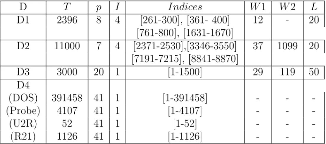
Table 5.1: Characteristics of Data Sets. D: Data sets. D1: Stock Indices, D2: Sensor, D3: MotorCurrent, D4: Network Traﬃc. T: total number of time stamps, p: dimensionality of the network data streams, I: total number of intervals for anomaly localization, Indices: starting point and ending point of the intervals for anomaly localization,W: total number of data windows for anomaly localization, W2: total number of data windows for anomaly detection L: sliding window size, -: not applicable.

D T p I Indices W1 W2 L D1 2396 8 4 [261-300], [361- 400] 12 - 20 [761-800], [1631-1670] D2 11000 7 4 [2371-2530],[3346-3550] 37 1099 20 [7191-7215], [8841-8870] D3 3000 20 1 [1-1500] 29 119 50 D4 (DOS) 391458 41 1 [1-391458] - - -(Probe) 4107 41 1 [1-4107] - - -(U2R) 52 41 1 [1-52] - - -(R21) 1126 41 1 [1-1126] - -

-The Stock Indices Data Set: The stock indices data set includes 8 stock market index streams from 8 countries: Brazil (Brazil Bovespa), Mexico (Bolsa IPC), Argentina (MERVAL), USA (S&P 500 Composite), Canada (S&P TSX Composite), HK (Heng Seng), China (SSE Composite), and Japan (NIKKEI 225). Each stock market index stream contains

(44)

2396 stamps recording the daily stock price indices from January 1st 2001 to March 5th 2010. Since this data set has no ground truth, we manually labeled all the daily indices for the selected intervals. In our labeling we followed the criteria list in [8] where small turbulence and co-movements of most markets are considered as normal, dramatic price changes or signiﬁcance deviation from the co-movement trend (e.g. one index goes up while the others in the market drop down) are considered as abnormal.

The Sun Spot Sensor Data Set: We collected a sensor data set in a car trial for transport chain security validation using seven wireless Sun Small Programmable Object Technologies (SPOTs). Each SPOT contains a 3-axis accelerometer sensor. In our data collection, seven Sun SPOTs were ﬁxed in separated boxes and were loaded on the back seat of a car. Each Sun SPOTs recorded the magnitude of accelerations along x, y, z axis with a sample rate of 390ms. We simulated a few abnormal events including box removal and replacement, rotation and ﬂipping. The overall acceleration √(x2 ₊_y2 ₊_z2_{) was used to}

detect the designed anomalous events.

The Motor Current Data Set: The Motor Current Data is the current observation generated by the state space simulations available at UCR Time Series Archive [29]. The anomalies are the simulated machinery failure in diﬀerent components of a machine. The cur-rent value was observed from 21 diﬀecur-rent motor operating conditions, including one healthy operating mode and 20 faulty modes. For each motor operating condition, 20 time series were recorded with a length of 1,500 samples. Therefore, there are 20 normal time series and 400 abnormal time series altogether.

In our evaluation, we randomly extracted 20 time series out of 420 with the length 1500. 10 time series are from normal series and the rest are from abnormal series. Hence A data matrix with size 1500×20 are used for anomaly localization. For anomaly detection, we concatenate the data matrix for anomaly localization with all the 20 normal series to make a new data matrix with size 3000×20.

A Family of Joint Sparse PCA Algorithms for Anomaly Localization in Network Data Streams