Classical and Bayesian Approach in Estimation of Scale Parameter of
Inverse Weibull Distribution
Kaisar Ahmad*, S.P. Ahmad* and A. Ahmed *Department of Statistics, University of Kashmir, Srinagar, India. Department of Statistics and O.R., Aligarh Muslim University, Aligarh, India.
Abstract: In this paper, Inverse Weibull Distribution is considered. The classical Maximum likelihood estimator has been obtained. Bayesian method of estimation has been employed in order to estimate the scale parameter of Inverse Weibull Distribution by using Jeffery’s and Quasi’s prior under three different loss functions. Also these methods are compared by using mean square error with varying sample sizes through simulation study conducted in R software.
Keywords: Inverse Weibull Distribution, Jeffrey’s and Quasi’s prior, loss functions and R software.
1. Introduction
The Weibull distribution is a very popular distribution named after Waloddi Weibull, a Swedish physicist. He applied this distribution in 1939 to analyze the breaking strength of materials. Since then, it has been widely used for analyzing lifetime data in reliability engineering. Many examples can be found among the aerospace, electronics, materials, and automotive industries. It can also be used as an alternative to Gamma and Log–normal distribution in reliability engineering and life testing. Some recent generalizations of Weibull distribution including the extended Weibull, modified Weibull are discussed in Pham et al. (2007). Zhang and Xie (2011) studied the characteristics and application of the truncated Weibull distribution which has a bathtub shaped hazard function.
The pdf of Weibull distribution can be increasing or decreasing or unimodel depending on the shape of the distribution parameters. Due to the flexibility of the Weibull pdf, the Inverse Weibull distribution (IWD) has been extensively employed in situations where the monotone data set is available. Furthermore, if the empirical studies indicate that the Weibull pdf might be unimodel, then the IWD may be appropriate model. In this paper classical and Bayesian method of estimation of (IWD) has been discussed.
If the random variable y0 has the Weibull Distribution with the following pdf f(y;,)y1exp(y) y0;, 0
Then the random variable y
x 1 has Inverse Weibull Distribution with the pdf of the form
( ;,) 1exp(x) x0;, 0 x
x
Where 0 and are
0 the scale and the shape parameters respectively. Graphical representation of pdf Inverse Weibull Distribution2. Materials and Methods:
There are two main philosophical approaches to statistics. The first is called the classical approach which was founded by Prof. R. A. Fisher in a series of fundamental papers round about 1930.
The alternative approach is the Bayesian approach which was first discovered by Reverend Thomas Bayes. In this approach, parameters are treated as random variables and data is treated fixed. An important pre-requisite in this approach is the appropriate choice of prior(s) for the parameters. Very often, priors are chosen according to ones subjective knowledge and beliefs. Recently this approach has received great attention by most researchers. Rahul et al. (2009) have discussed the application of Bayesian methods. The other integral part of Bayesian inference is the choice of loss function. Various authors have used symmetric and asymmetric loss functions (for details see; see Varian (1975), Zellner (1986) and S.P. Ahmad and Kaisar Ahmad (2013) and Kaisar et al. (2015 a, b)) etc.
Theorem 2.1:- Let (x1,x2,...,xn) be a random sample of size n having pdf (1.1), then the
maximum likelihood estimator of scale parameter , when the shape parameter
is known, is given by
n i i x n 1 ˆ Proof: - The likelihood function of the pdf (1.1) is given by
0 2 4 6 8 10 12 0 .0 0 .1 0 .2 0 .3 0 .4 Figure
1:The pdf's of Inverse Weibull distribution under various values of alpha and beta x f( x) alpha=1.0,beta=1.0 alpha=1.0,beta=1.5 alpha=1.5,beta=1.0 alpha =1.5,beta=1.5 alpha =2.0,beta=1.0 alpha =2.0,beta=1.5
( ; , ) ( ) 1 1 1
n i i x n i i n e x x L (2.1.1)The log likelihood function is given by
n i i n i i x x n n x L 1 1 * log 1 log log ) , ; ( log (2.1.2)Differentiating (2.1.2) w.r.t. to and equate to zero, we get
n i i x n 1 ˆ (2.1.3)2.2 Loss functions used in this paper: (i)Linex Loss function:
For obtaining the Bayesian estimate of scale parameter 𝛼 we use a very useful asymmetric linex loss function given by
L()
exp(c)c1
, where (ˆ) Where and ˆ represent the true and estimated values of the parameter.(ii) Precautionary Loss function: The precautionary loss function (For details, see Norstrom (1996)) is given by
ˆ ˆ , ˆ 2 pr lWhere and ˆ represent the true and estimated values of the parameter.
(iii) Al-Bayyati’s loss function:
The Al-Bayyati’s loss function is given by l
ˆ,
c1
ˆ
2; c1 R.A
which is an asymmetric loss function, andˆ represents the true and estimated values of the parameter.
3. Bayesian Method of Estimation: 3.1 Posterior density under Jeffreys’ prior:
Let (x1,x2,,xn) be a random sample of size n having the probability density function (1.1) and
the likelihood function (2.1.1).
g() det(I())
Where is k-vector valued parameter and I() is the Fisher’s information matrix of order
. k k Thus k g( ) (3.1.1) where k is a constant.
The posterior distribution of is given by
1
|x
L(x|)g() (3.1.2)Using (2.1.1) and (3.1.1) in (3.1.2), we get
n i i x n e k x 1 1 1 | (3.1.3) and n x k n n i i
1 Using the value of k in (3.1.3)
n e x x n i i x n n i i n 1 1 1 1 | (3.1.4)3.2 Posterior density under Quasi prior:
Let (x1,x2,,xn) be a random sample of size n having the pdf (1.1) and the likelihood function (2.1.1).
We consider the prior distribution of to be
0 , 1 ) ( where d g d (3.2.1) The posterior distribution of is given by
2
|x
L(x|)g() (3.2.2)Using (2.1.1) and (3.2.1) in (3.2.2), we get
n i i x d n e k x 1 | 2 (3.2.3) Where k is independent of .and ) 1 ( 1 1
d n x k d n n i i By using the value of k in (3.2.3), we get
) 1 ( | 1 1 1 2 d n e x x n i i x d n n i i d n (3.2.4)4. Bayesian estimation by using Jeffreys’ prior under different Loss Functions: Theorem 4.1:- Assuming the loss functionLln
ˆ,
, the Bayes estimate of the scale parameter, if the shape parameter
is known, is of the form
n i i x c c n 1 1 log ˆ Proof: - The risk function of the estimatorunder the linex loss function Lln
ˆ,
is given by the formula R
ˆ exp(c(ˆ )) c(ˆ ) 1
1|x
d 0
(4.1.1) Using (3.1.4) in (4.1.1), we have
d n e x c c R n i i x n n i i n
1 1 1 0 1 ) ˆ ( )) ˆ ( exp( ˆ (4.1.2) On solving (4.1.2), we have
ˆ ˆ 1) 1 1 1 1
n n i i n n i i n n i i x n n c c x c x R
n i i x c c n 1 1 log ˆ (4.1.3)Theorem 4.2:- Assuming the loss functionLpr
ˆ,
, the Bayes estimate of the scale parameter , if the shape parameter
is known, is of the form
n i i x n n 1 ) 1 ( ˆ Proof: - The risk function of the estimatorunder precautionary loss function Lpr
ˆ,
is given by the formula
x d R | ˆ ) ˆ ( ˆ 1 0 2
(4.2.1) Using (3.1.4) in (4.2.1), we have
d n e x R n x n i i n n i i
1 1 1 0 2 ˆ ) ˆ ( ˆ (4.2.3) On solving (4.2.3), we have
n i i n i i n x n x n n R 1 2 1 ) 1 ( 2 ˆ ) 2 ( ˆ ˆ Minimization of the risk with respect to ˆ gives us the optimal estimator
n i i x n n 1 ) 1 ( ˆ (4.2.3)Theorem 4.3:- Assuming the loss functionLAl
ˆ,
, the Bayes estimate of the scale parameter , if the shape parameter
is known, is of the form
n i i x c n 1 1) ( ˆ Proof: - The risk function of the estimatorunder Al-Bayyati’s loss function LAl
ˆ,
is given by the formulaR
ˆ c
ˆ
1 |x
d 0 2 1
(4.3.1) Using (3.1.4) in (4.3.1), we have
d n e x R n i i x n n i i n c
1 1 1 1 0 2 ˆ ˆ (4.3.2) On solving (4.3.2), we have
1 1 1 2 1 1 1 1 2 1 1 1 ) 1 ( ˆ 2 ) 2 ( ) ( ˆ ˆ
n c i i c n i i c n i i n x c n x n c n x n c n R Minimization of the risk with respect to ˆ gives us the optimal estimator
n i i x c n 1 1) ( ˆ (4.3.3)Table 4a: Estimates using Jeffreys’ prior under different loss functions
n ML ln pr Al C1=0.5 C1=1 25 0.5 1.0 0.05435046 0.05224848 0.07686316 0.08152569 0.1087009 1.0 1.5 0.0004761753 0.0004760053 0.0006734136 0.000714263 0.0009523506 50 0.5 1.0 0.02772421 0.02716323 0.03920795 0.04158631 0.05544841 1.0 1.5 8.461315e-05 8.460778e-05 0.0001196611 0.0001269197 0.0001692263 100 0.5 1.0 0.01400142 0.01385642 0.019801 0.02100213 0.02800284
1.0 1.5 1.498501e-05 1.498484e-05 2.1192e-05 2.247751e-05 2.997001e-05
Table 4b: MSE using Jeffrey’s prior under different loss functions
ML=Maximum Likelihood, ln=Linex loss function, Pr=Precautionary loss function, Al= Al-Bayyati’s loss function
n ML ln pr Al C1=0.5 C1=1 25 0.5 1.0 0.3281245 0.3248216 0.303385 0.2994609 0.2774552 1.0 1.5 1.06243 1.059895 1.0595 1.059418 1.058943 50 0.5 1.0 0.2752069 0.2746938 0.2634485 0.2612623 0.2487453 1.0 1.5 1.017244 1.016896 1.016826 1.016811 1.016727 100 0.5 1.0 0.2883312 0.2819536 0.2762091 0.275057 0.2683994 1.0 1.5 1.01055 1.010444 1.010431 1.010429 1.010414
5. Bayesian estimation by using Quasi prior under different Loss Functions:
Theorem 5.1:- Assuming the loss functionLln
ˆ,
, the Bayes estimate of the scale parameter, if the shape parameter
is known, is of the form
n i i x c c d n 1 1 log 1 ˆ Proof: - The risk function of the estimatorunder the linex loss function Lln
ˆ,
is given by the formula R
ˆ exp(c(ˆ )) c(ˆ ) 1
2 |x
d 0
(5.1.1) Using (3.1.4) in (4.1.1), we have
d d n e x c c R n i i x d n n i i d n
exp( (ˆ )) (ˆ ) 1 ( 1) ˆ 1 1 1 0 (5.1.2) On solving (5.1.2), we have
ˆ ( 1) 1 ) ˆ exp( ˆ 1 1 1 1 1
n i i d n n i i d n n i i x d n c c x c x c R Minimization of the risk with respect to ˆ gives us the optimal estimator
n i i x c c d n 1 1 log 1 ˆ (5.1.3)Remark: Replacing d=1 in (5.1.3), the same Bayes estimator is obtained as in (4.1.3) corresponding to the Jeffrey’s prior.
Theorem 5.2:- Assuming the loss functionLpr
ˆ,
, the Bayes estimate of the scale parameter, if the shape parameter
is known, is of the form
n i i x d n d n 1 ) 2 )( 1 ( ˆ Proof: - The risk function of the estimatorunder precautionary loss function Lpr
ˆ,
is given by the formula
x d R | ˆ ) ˆ ( ˆ 2 0 2
(5.2.1) Using (3.2.4) in (5.2.1), we have
d d n e x R n i i x d n n i i d n
(ˆ ˆ ) ( 1) ˆ 1 1 1 0 2 (5.2.2) On solving (5.2.2), we have
n i i n i i n d x d n x d n d n R 1 2 1 ) 1 ( ) 2 ( 2 ) 1 ( ˆ ) 3 ( ˆ ˆ Minimization of the risk with respect to ˆ gives us the optimal estimator
n i i x d n d n 1 ) 2 )( 1 ( ˆ (5.2.3)Remark: Replacing d=1 in (5.2.3), the same Bayes estimator is obtained as in (4.2.3) corresponding to the Jeffrey’s prior.
Theorem 5.3:- Assuming the loss functionLAl
ˆ,
, the Bayes estimate of the scale parameter , if the shape parameter
is known, is of the form
n i i x d c n 1 1 1) ( ˆ Proof: - The risk function of the estimatorunder Al-Bayyati’s loss function LAl
ˆ,
is given by the formulaR
ˆ c
ˆ
2 |x
d 0 2 1
(5.3.1) Using (3.2.4) in (5.3.1), we have
d d n e x R n i i x d n n i i d n c
ˆ ( 1) ˆ 1 1 1 1 0 2 (5.3.2) On solving (5.3.2), we have
1 1 1 2 1 1 1 1 2 1 1 1 ) 1 ( ) 2 ( ˆ 2 ) 1 ( ) 3 ( ) 1 ( ) 1 ( ˆ ˆ
n c i i c n i i c n i i n d x d c n x d n d c n x d n d c n R Minimization of the risk with respect to ˆ gives us the optimal estimator
n i i x d c n 1 1 1) ( ˆ (5.3.3)Remark: Replacing d=1 in (5.3.3), the same Bayes estimator is obtained as in (4.3.3) corresponding to the Jeffrey’s prior.
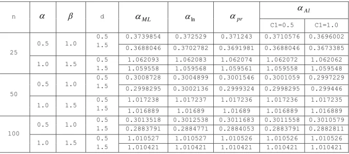
Table 5a: Estimates using Quasi prior under different loss functions
n d ML ln pr Al C1=0.5 C1=1.0 25 0.5 1.0 0.5 1.5 0.002953972 0.004421171 0.005720343 0.005907945 0.007384931 0.002953972 0.001473724 0.002558215 0.002953972 0.004430958 1.0 1.5 0.5 1.5
1.039083e-05 1.558613e-05 2.012176e-05 2.078166e-05 2.597708e-05 1.039083e-05 5.195376e-06 8.998724e-06 1.039083e-05 1.558625e-05
50
0.5 1.0 0.5 1.5 0.0007686316 0.001152283 0.001488449 0.001537263 0.001921579 0.0007686316 0.0003840944 0.0006656544 0.0007686316 0.001152947 1.0 1.5 0.5 1.5 7.783175e-07 1.167476e-06 1.507205e-06 1.556635e-06 1.945794e-06
7.783175e-07 3.891585e-07 6.740428e-07 7.783175e-07 1.167476e-06 100 0.5 1.0 0.5 1.5 0.0001960397 0.0002940164 0.0003796293 0.0003920795 0.0004900993 0.0001960397 9.800546e-05 0.0001697754 0.0001960397 0.0002940596 1.0 1.5 0.5 1.5
5.800767e-08 8.701151e-08 1.123314e-07 1.160153e-07 1.450192e-07 5.800767e-08 2.900384e-08 5.023612e-08 5.800767e-08 8.701151e-08
Table 5b: MSE using Quasi prior under different loss functions n d ML ln pr Al C1=0.5 C1=1.0 25 0.5 1.0 0.5 1.5 0.3739854 0.372529 0.371243 0.3710576 0.3696002 0.3688046 0.3702782 0.3691981 0.3688046 0.3673385 1.0 1.5 0.5 1.5 1.062093 1.062083 1.062074 1.062072 1.062062 1.059558 1.059568 1.059561 1.059558 1.059548 50 0.5 1.0 0.5 1.5 0.3008728 0.3004899 0.3001546 0.3001059 0.2997229 0.2998295 0.3002136 0.2999324 0.2998295 0.299446 1.0 1.5 0.5 1.5 1.017238 1.017237 1.017236 1.017236 1.017235 1.016889 1.01689 1.01689 1.016889 1.016889 100 0.5 1.0 0.5 1.5 0.3013518 0.3012538 0.3011683 0.3011558 0.3010579 0.2883791 0.2884771 0.2884053 0.2883791 0.2882811 1.0 1.5 0.5 1.5 1.010527 1.010527 1.010526 1.010526 1.010526 1.010421 1.010421 1.010421 1.010421 1.010421 ML=Maximum Likelihood, ln=Linex loss function, Pr=Precautionary loss function, Al= Al-Bayyati’s loss function
6. Results and Discussion:-
We primarily studied the Classical Maximum Likelihood estimation and Bayesian estimation for Inverse Weibull Distribution using Jeffreys’ and Quasi priors under three different loss functions.
For descriptive manner, we generate different random samples of size 25,50 and 100 to represent small, medium and large data set for the Inverse Weibull Distribution in R Software, a simulation study was carried out 3,000 times for each pairs of
,
where
0.5,1.0
and
1.0,1.5
.The values of extension were (d=0.5, 1.5). The value for the loss parameter (C1 =0.5 and 1.0).This was iterated 2000 times and the estimates of scale parameter for each method were calculated. The results are presented in tables (4a, 4b, 5a and 5b) respectively. In table 4b, Bayes estimate using Jeffrey’s prior under Al-Bayyati’s Loss function provides the smallest values in most cases as compared to other loss functions and classical maximum likelihood estimator especially when loss parameter C1 is 1.0.In table 5b, Bayes estimate using Quasi prior under Al-Bayyati’s Loss function provides the smallest values in most cases as compared to other loss functions and classical maximum likelihood estimator especially when loss parameter C1 is 1.0.
7. Conclusion:-
From the above results, we observe that Bayes estimate under Al-Bayyati’s Loss function has the smallest Mean Squared Error (MSE) values for both prior’s (Jeffrey’s and Quasi prior) as compared to other loss functions and classical maximum likelihood estimator especially when
loss parameter C1 is 1. Thus we can conclude that Bayes estimate under Al-Bayyati’s Loss function is efficient.
References:
1. Ahmad, S.P. and Kaisar Ahmad (2013). Bayesian Analysis of Weibull Distribution Using R Software “Australian Journal of Basic and Applied Sciences, 7(9): 156-164. ISSN 1991-8178.
2. Hoang Pham and Chin-Diew Lai (2007): On Recent Generalizations of the Weibull Distribution. IEEE Transactions on RELIABILITY, 56(3):454–458.
3. Jefferys, H. (1946). An invariant form for the prior probability in estimation problems; proceedings of the royal Society of London, Series. A. 186, 453-461.
4. Kaisar Ahmad, S.P. Ahmad and A. Ahmed (2015 a): On parameter estimation of Erlang Distribution using Bayesian method under different loss functions. Proceedings of international conference on Advances in Computers, Communication, and Electronic Engineering held March 16-18, 2015, pp 200-206. University of Kashmir. ISBN: 978-93-82288-54-1.
5. Kaisar Ahmad, S.P. Ahmad and A. Ahmed (2015 b): Bayesian Analysis of Generalized Gamma Distribution using R Software. Journal of Statistics Applications & Probability, J. Stat. Appl. Pro. 4, No. 2, 323-335.
6. Norstrom, J. G. (1996). The use of Precautionary Loss Functions in Risk Analysis. IEEE Transactions on reliability, (3), 400-403.
7. Rahul, G. P., Singh and O.P. Singh, (2009): Population project OF Kerala using Bayesian methodology .Asian J. Applied Sci., 2: 402-413.
8. Varian, H. R. (1975). A Bayesian approach to real estate assessment, Studies in Bayesian Econometrics and Statistics in Honor of Leonard J. Savage (eds: S.E. Fienberg and A.Zellner), North-Holland, Amsterdam, 195-208.
9. Zellner, A., (1986): Bayesian estimation and prediction using asymmetric loss function. Journal of American Statistical Association exponential distribution using simulation. Ph.D Thesis, Baghdad University, Iraq. 81, 446-451.
10.Zhang T, Xie M. (2011): On the upper truncated Weibull distribution and its reliability implications. Reliability Engineering System Safety; 96(1):