Multicore processors and graphics processing unit accelerators for parallel retrieval of aerosol optical depth from satellite data: implementation, performance, and energy efficiency

(1)

T

Multicore Processors and Graphics Processing Unit

Accelerators for Parallel Retrieval of Aerosol Optical

Depth From Satellite Data: Implementation,

Performance, and Energy Efficiency

Jia Liu, Dustin Feld, Yong Xue, Senior Member, IEEE, Jochen Garcke, and Thomas Soddemann

Abstract—Quantitative retrieval is a growing area in remote sensing due to the rapid development of remote instruments and retrieval algorithms. The aerosol optical depth (AOD) is a significant optical property of aerosol which is involved in fur- ther applications such as the atmospheric correction of remotely sensed surface features, monitoring of volcanic eruptions or for- est fires, air quality, and even climate changes from satellite data. The AOD retrieval can be computationally expensive as a result of huge amounts of remote sensing data and compute-intensive algorithms. In this paper, we present two efficient implementa- tions of an AOD retrieval algorithm from the moderate reso- lution imaging spectroradiometer (MODIS) satellite data. Here, we have employed two different high performance computing architectures: multicore processors and a graphics processing unit (GPU). The compute unified device architecture C (CUDA-C) has been used for the GPU implementation for NVIDIA’s graphic cards and open multiprocessing (OpenMP) for thread- parallelism in the multicore implementation. We observe for the

Manuscript received September 02, 2014; revised April 08, 2015; accepted May 25, 2015. Date of publication June 10, 2015; date of current version July 20, 2015. This work was supported in part by the Ministry of Science and Technology (MOST), China under Grant 2013AA122801, Grant 2010CB950802, and Grant 2013CB733403, in part by the National Natural Science Foundation of China (NSFC) under Grant 41271371, in part by the Institute of Remote Sensing and Digital Earth Institute, Chinese Academy of Sciences (CAS-RADI) Innovation project under Grant Y3SG0300CX, in part by the Joint Doctoral Promotion Program hosted by Fraunhofer Institute and Chinese Academy of Sciences, and in part by the graduate foundation of CAS-RADI under Grant Y4ZZ06101B. (Corresponding author: Yong Xue.)

J. Liu is with the Key Laboratory of Digital Earth Science, Institute of Remote Sensing and Digital Earth, Chinese Academy of Sciences, Beijing 100094, China, also with Fraunhofer Institute for Algorithms and Scientific Computing (SCAI), 53754 Sankt Augustin, Germany, and also with the University of Chinese Academy of Sciences, Beijing 100049, China (e-mail: [email protected]).

D. Feld is with the Fraunhofer Institute for Algorithms and Scientific Computing (SCAI), 53754 Sankt Augustin, Germany, and also with the Department of Computer Science, University of Cologne, 50923 Cologne, Germany.

Y. Xue is with the Key Laboratory of Digital Earth Science, Institute of Remote Sensing and Digital Earth, Chinese Academy of Sciences, Beijing 100094, China, and also with the Faculty of Life Sciences and Computing, London Metropolitan University, London N7 8DB, U.K. (e-mail: xueyong@ radi.ac.cn).

J. Garcke is with Fraunhofer Institute for Algorithms and Scientific Computing (SCAI), 53754 Sankt Augustin, Germany, and also with the Institute for Numerical Simulation, University of Bonn, 53115 Bonn, Germany. Soddemann is with the Fraunhofer Institute for Algorithms and Scientific Computing (SCAI), 53754 Sankt Augustin, Germany.

Color versions of one or more of the figures in this paper are available online at http://ieeexplore.ieee.org.

Digital Object Identifier 10.1109/JSTARS.2015.2438893

GPU accelerator, a maximal overall speedup of 68.x for the studied data, whereas the multicore processor achieves a reasonable 7.x speedup. Additionally, for the largest benchmark input dataset, the GPU implementation also shows a great advantage in terms of energy efficiency with an overall consumption of 3.15 kJ compared to 58.09 kJ on a CPU with 1 thread and 38.39 kJ with 16 threads. Furthermore, the retrieval accuracy of all implementations has been checked and analyzed. Altogether, using the GPU accelera- tor shows great advantages for an application in AOD retrieval in both performance and energy efficiency metrics. Nevertheless, the multicore processor provides the easier programmability for the majority of today’s programmers. Our work exploits the par- allel implementations, the performance, and the energy efficiency features of GPU accelerators and multicore processors. With this paper, we attempt to give suggestions to geoscientists demanding for efficient desktop solutions.

Index Terms—Aerosol optical depth (AOD), graphics process- ing unit (GPU), High performance computing (HPC), OpenMP, quantitative remote sensing retrieval.

I. INTRODUCTION

HE CONTINUOUS increase of spatial and spectral resolution of satellite sensors over the last years has led to a substantial increase in data volumes, and this trend is expected to continue in the future [1]. For instance, the Moderate Resolution Imaging Spectroradiometer (MODIS) instruments with 36 spectral bands and 12-bit radiometric resolution on- board the Earth Observing System (EOS) satellite TERRA and AQUA have been widely used for over 10 years after being successfully launched in December 1999 and May 2002, respectively. Large numbers of multidisciplinary geophysical parameters are produced by each observation, thus the MODIS Adaptive Processing System (MODAPS) was developed. It pro- duces nearly 2.5 TB of data from land, atmosphere and ocean measurements [2]. To retrieve a 10-year aerosol optical depth (AOD) dataset at 1-km spatial resolution using the synergetic retrieval of aerosol properties model from the MODIS data (SRAP-MODIS), the input MODIS data acquired is expected to sum up to 29 TB [3]. As a result, efficient processing and analysis of the time series data accumulated from the multi- source satellite instruments is crucial. In addition, this data are also required for real-time or near real-time response in several other applications such as the monitoring of volcanic eruptions or forest fires. With a growing amount of data and an increasing complexity of its processing, as well as for solving models with 1939-1404 © 2015 IEEE. Translations and content mining are permitted for academic research only. Personal use is also permitted, but republication/redistribution

(2)

i,j i,j j i j

j j

it, the demand for computing power increases significantly in this field.

There are research efforts toward the incorporation of high performance computing (HPC) technologies and practices into the remote sensing community to address the aforementioned computing needs. Lee et al. reviewed the recent developments in HPC for remote sensing in 2011 and summarized them into three categories: 1) specialized hardware architectures including field programmable gate arrays (FPGAs) and graphics processing units (GPUs); 2) cluster computing including traditional Beowulf cluster and clusters based on hardware accelerators; and 3) distributed computing infrastructures [4]. Generally, remote sensing applications map relatively nicely to clusters and networks of computers; therefore, development efforts have been made to accelerate remote sensing applications by using cluster, grid, and cloud infrastructures [5]–[7]. Unfortunately, these systems require major investments in working time and finances for their maintenance and it is difficult to adapt them to on-board satellite or aircraft processing scenarios due to their large space occupation [8], [9]. Therefore, low-weight integrated components such as FPGAs have come up as feasible alternatives. However, making use of them requires significant efforts with regard to code-design and programmability. The multicore processors and commod- ity GPUs are promising options, especially for recent desktop and server-based processing, in future even for on-board solutions. They offer very substantial computational power at low cost and therefore provide the chance to bridge the gap toward fast or even real-time data processing and analysis for remote sensing applications [9].

So far, great efforts have already been put into the acceleration of hyperspectral remote sensing based on GPUs and multicore platforms. For instance, Torti et al. presented new parallel implementations of the widely used hyperspectral subspace identification employing minimum error algorithm on GPUs, multicore processors, and digital signal processors (DSPs), and obtained real-time performance with the GPU and multicore implementations [10]. Molero et al. exploited the computational power of GPUs and multicore processors for anomaly detection using hyperspectral data. They also measured the average power intake of implementations and calculated the energy consumptions [11]. Bernabe et al. developed efficient implementations of a full hyperspectral unmixing chain on GPUs and multicore processors and gave a detailed comparison in terms of performance, costs, and mission payload [9]. In addition to research on the acceleration of hyperspectral remote sensing algorithms, GPUs and multicore processors have also been utilized for a few quantitative remote sensing applications. Efremenko et al. developed and compared multicore and GPU implementations of a radiative transfer model based on the discrete ordinate solution method [12]. Su et al. proposed a GPU implementation for the Monte-Carlo-based electromagnetic scattering of a double-layer vegetation model [13]. For Infrared Atmospheric Sounding Interferometer (IASI) in operational numerical weather prediction systems, Mielikainen et al. developed a GPU-based radiative transfer model [14]. There

using hyperspectral data employing GPU accelerators [11]. Nevertheless, a study of performance versus energy consumption on both multicore and GPU platforms, in the field of remote sensing quantitative retrieval has, to the best of our knowledge, not yet been conducted.

In this paper, we focus on two different kinds of parallel desktop architectures: multicore processors and GPU accelerators. We implemented the time-consuming SRAP-MODIS algorithm for the retrieving of AOD. It not only employs a set of nonlinear equations but also requires a large set of input images. The GPU implementation was carried out based on compute unified device architecture C (CUDA-C) for NVIDIA GPUs, while the multicore implementation was realized using open multiprocessing (OpenMP). Furthermore, we measured and analyzed the obtained accuracy for both considered platforms. Their parallel performance and energy consumption were compared in the context of a quantitative remote sensing retrieval application.

This paper is organized as follows. Section II explains the SRAP-MODIS algorithm and the multicore as well as the GPU accelerated implementations. Section III describes the satellite remote sensing data and the benchmark environment for our experiments and presents an experimental evaluation of the proposed implementations in terms of the retrieval accuracy, parallel performance, energy consumption, and coding considerations. Finally, Section IV concludes with remarks and future research perspectives.

II. METHODOLOGY

A. AOD Retrieval Algorithm From MODIS Satellite Data AOD is defined as the integrated extinction coefficient over a vertical column of unit cross section. The extinction coefficient is the fractional depletion of radiance per unit path length. AOD represents the degree to which aerosols prevent the transmis- sion of light by absorption or scattering of light and therefore, it is of interest to several applications such as the atmospheric correction of remotely sensed surface features, the monitoring of volcanic eruptions or forest fires, air quality, health and environment, earth radiation budget, and climate change [16]– [20]. Many approaches have been developed for the retrieval of AOD, including the use of advanced very high resolution radiometer (AVHRR), medium resolution imaging spectrometer (MERIS), scanning imaging absorption spectrometer for atmospheric chartography (SCIAMACHY), MODIS, multian- gle imaging spectro radiometer (MISR), advanced along-track scanning radiometer (AATSR), and others [21].

SRAP-MODIS is a simple but practical algorithm that was introduced in the research of [22] on an operational bi-angle approach model for retrieving AOD and the earth surface reflectance [23]. The algorithm employs a set of nonlinear equations which can be written as

Ai,j =

(aAj₋_b₎₊_b₍₁₋_Aj _)exp[_ε₍_b₋_a₎₍₀_.₀₈₇₉_λ−4.09₊_{β λ}−α₎_bj_] energy consumption for hyperspectral unmixing algorithms on

multicore platforms [15] as well as for the anomaly detection

(aAj_i,j₋_b₎₊_a₍₁₋_Aj_i,j_)exp[_ε₍_b₋_a₎₍₀_.₀₈₇₉_λ−4.09₊_β_i_λ−α₎_bj_]

(1) have also been endeavors to analyze the performance and

(3)

j_A

j where Ai,jobserves the constraints (2)

A1,j A2,j Aj 1,λ=2.12 µm = 2,λ=2.12 µ m (2) where i = 1, 2 represents the observations of satellite TERRA MODIS and AQUA MODIS, respectively, j = 1, 2, 3 stands for three visible spectral bands at central wavelengths of 470, 550, and 660 nm. Hence, a set of nonlinear equations consisting of three equations is formed. The unknowns to be solved are β1, β2, and α, which are then used to calculate AOD according to the Angstrom’s turbidity formula

τA = βiλ−α. (3)

The other variables in (1) can be derived from the satellite image data after preprocessing. More details can be found in [3]. The input image datasets required by the SRAP-MODIS retrieval part include:

1) The top of atmosphere reflectance information which is extracted and preprocessed through georeferencing, water vapor and ozone absorption correction, and cloud mask from the MOD/MYD021KM—Level 1B Calibrated Radiances—1 km from both the TERRA and AQUA MODIS.

2) The angles and geolocation information for georeference from MOD/MYD03—Geolocation—1 km.

3) The MOD/MYD04_L2—Level 2 Aerosol Products. 4) The parameter text including the longitude and latitude

information of retrieval spatial coverage, the spatial resolution and others.

The satellite data from the MODIS instrument can be downloaded from the Level 1 and Atmosphere Archive and Distribution System (LAADS Web) supported by the National Aeronautics and Space Administration (NASA) Goddard Space Flight Center [24].

B. Implementation for Multicore Processors

A multicore processor is a single computing component with two or more independent processor-cores. For quite a while now, one sees only modest increases in clock speed for compute cores since physical limitations make it extremely difficult to increase CPU performance on this end. Going multicore and increasing the performance of the CPU’s internal func- tional units, e.g., better vector units with longer vectors such as advanced vector extensions (AVX), seems, at least for now, to be the way to go. Hence, programs have to adhere to these levels of parallelism introduced with the hardware to leverage the performance gain of modern CPUs.

In our multicore implementation of the AOD retrieval, we used OpenMP which has established itself as the standard for shared-memory parallel programming [25]. OpenMP is an application programming interface (API) based on compiler directives available for C, C++, and FORTRAN to exploit shared-memory parallelism. It is based on the fork-join model and processes parallel regions where computational work is shared and spread across multiple threads. The main part of the

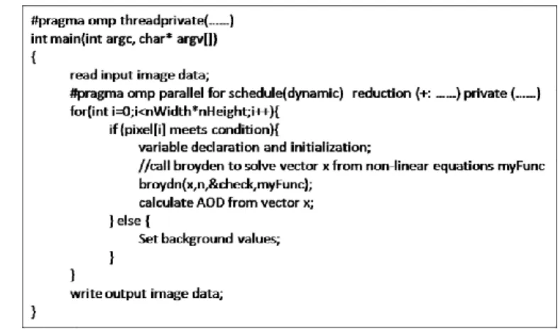
Fig. 1. Pseudo-code for the multicore implementation.

multicore implementation is given in the pseudo-code in Fig. 1. The main techniques used in our implementation of the AOD retrieval are summarized and explained as follows.

1) In our SRAP-MODIS AOD retrieval procedure, there is a set of equations to be solved to calculate the AOD from the solution and input parameters for each pixel inside the prospected images. The calculation of the AOD according to (1)–(3) is for each pixel independent from all other pixels. Note that we use Broyden’s method to solve the nonlinear equations, more technical details are given in Section III-C.

2) Each pixel is treated entirely by one thread within a parallel for loop to solve its equations and perform the AOD calculations. Each thread executes the same instruction stream with multiple data. There is implicit barrier syn- chronization at the end of the parallel region, a block of code executed by multiple threads, under the directive parallel for before the resulting images are written. 3) To tune the performance of the multicore code, we care-

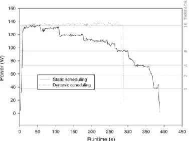
fully investigated the impact of the underlying OpenMP scheduling strategy. Fig. 2 shows that the implementation using OpenMP in the standard configuration with static scheduling can lead to an extremely unbalanced work- load among the cores. The energy profile brings to light that over time more and more cores become idle as they are statically served with a fixed amount of iterations. As soon as a thread finishes all of its iterations, it is not served with additional work and is therefore not utilized for the rest of the execution. The unbalance among the threads is based on the facts that a) the algorithm has a pixel-based nature; b) cloudy pixels which follow a different control flow than “normal” ones are usually located in continuous parts within an image and therefore are often assigned onto the same core within the parallel calculation; and c) even certain cloud-free pixels’ iterations finish quicker than others. Thus, the performance with a static scheduling depends significantly on the pixels’ distribution to the cores. To overcome this imbalance, a dynamic scheduling strategy was used with OpenMP. Fig. 2 shows that this leads to a uniform usage of all cores during the whole execution of the program and, as a result, to shorter runtimes (see Fig. 3). We give more details on the runtime

(4)

Fig. 2. Energy comparison of the static scheduling and dynamic scheduling for the multicore implementation.

Fig. 3. Performance comparison of the static scheduling and dynamic scheduling for the multicore implementation.

and also the energy consumption behaviour of the codes in Sections III-D and III-E.

4) The local and global variables corresponding to multiple input parameters for solving the equation are kept in the private and threadprivate lists.

C. Implementation for GPUs

GPUs have in recent years evolved into highly parallel, multithreaded, many-core processors with tremendous computational speed and very high memory bandwidth [4]. Therefore, they are well suited for massively data parallel processing with high arithmetic floating point intensity. With the dramatic increase of the processing power of GPUs, it is possible to use GPUs for efficient general purpose processing nowadays [26], namely in the field of general purpose GPU (GPGPU) computing.

Fig. 4. CUDA hierarchy of threads, blocks, and grids, with corresponding per-thread private, per-block shared, and per-application global memory spaces [35].

CUDA and the open computing language (OpenCL) are the two main basic approaches for allowing general purpose programming of GPUs. Taking into account that the GPU device we are using is Tesla K20 from NVIDIA, and since early com- parisons of CUDA and OpenCL suggest CUDA is consistently faster than OpenCL using complex, near-identical kernels [27] and equivalent implementations on the same hardware [26], we decided to use CUDA for our GPU implementation of the AOD retrieval.

The CUDA architecture enables NVIDIA GPUs to exe- cute parallel programs. A CUDA program executes kernels in parallel across a set of parallel threads organized in thread blocks and grids consisting of those thread blocks as shown in Fig. 4. Correspondingly, Fig. 4 also presents different levels of memory, i.e., registers and local memory for a thread, shared memory for the block and global as well as constant memory and texture memory for the grid on the GPU. The GPU instan- tiates a kernel program on a grid of thread blocks, whereas each thread within a thread block executes an instance of the kernel. The flowchart of the AOD retrieval supported by CPU and GPU collaboratively is shown in Fig. 5. The CUDA kernel and the main part of the GPU implementation are given in pseudo-code in Fig. 6. The main implementation techniques and strategies are described as follows.

1) A CUDA kernel called “retrievalOfAOD” was designed and implemented to solve (1)–(3) and calculate AOD as a whole with 15 input image bands, 6 output image bands, and several necessary parameters, e.g., the pictures’ width and size.

2) Each thread corresponds to the computation of the AOD calculation of one pixel using the CUDA kernel “retrieval- OfAOD.”

(5)

×

× × × × × Fig. 5. Flowchart of the CUDA implementation.

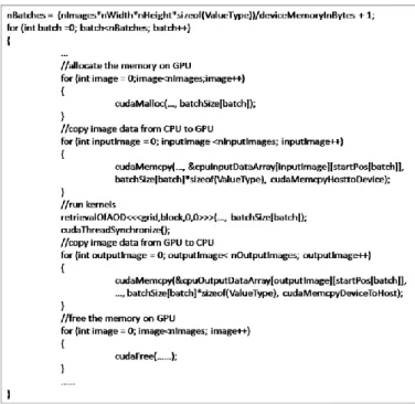
Fig. 6. Pseudo-code for the GPU implementation including the CUDA kernel.

3) The image data is organized as a one-dimensional float type array, and the pixels are mapped to threads inside the CUDA kernel “retrievalOfAOD” as shown in Fig. 6.

Fig. 7. Image data split pattern for images that do not fit into the GPU’s memory at once. This is a sketch of how the splitting can be realized including data-transfers, etc., when using a GPU. Calculation and data-transfer could additionally be overlapped by a double-buffering with halved batchSize per load running asynchronously on two CUDA streams.

4) The global memory is used to store the input and output image data directly on the GPU. For the largest image in our experiments, which contains 11 500 4500 pixels, the 21 image bands demand slightly over 4 GB memory. For the Tesla K20 device with 5 GB memory, the image can be copied between host and GPU memory back and forth at once, while the image data would have to be split from the spatial domain when the memory of the GPU device is smaller than the image data size. Such an approach can also be advantageous on CPUs to prevent cache misses or even paging. The split pattern can be performed as shown in Fig. 7. A few temporary variables in the procedure of solving the nonlinear equations are kept in registers for the threads for faster access.

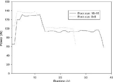
5) To tune the performance of our GPU implementation, we analyzed the impact of the thread-block configuration on the runtime. The largest number of threads per block is 256 for our implementation on a Tesla K20 with compute capability 3.5 when taking the compiler chosen number of registers (114 registers per thread). We therefore measured the runtime for all input sizes on a two-dimensional block of 1 1, 2 2, 4 4, 8 8, and 16 16 threads, while the dimensions of the grid are set dynamically corresponding to the image size as shown in Fig. 6 inside the main function using the dim3 block and the dim3 grid. The best performance is achieved when executing with 8 8 threads per block (see Fig. 8). Fig. 9 shows that this configuration results in a slightly higher power intake than with the maximum of 16 16 threads, but in exchange to a much shorter runtime and, thus, also to a significantly less overall energy consumption.

(6)

× × × × × × × × × × × × × × ×

Fig. 8. Impact of block sizes on the runtime for the GPU implementation.

Fig. 9. Energy comparison of the block size 8 8 and 16 16 for the GPU implementation.

6) Fixing the optimal 8 8 thread-block size, we varied the registers per thread by the nvcc option (maxrregcount amount) from 50 to 255, the maximum for K20, the relative improvement is shown in Fig. 10. As compared to the compiler’s internal decision (which uses registers/thread = 114), the experiments show that none of those configurations lead to a significant improvement of the runtime for all of the prospected codes with 8 8 threads. Decreasing the maximum number of registers per thread however allows executing more parallel threads. For example, restricting the compiler to use only half the number of registers (57) allows using 32 32 threads. Even though this increases the amount of parallelism, data has to be served from slower memory than the register- memory. Hence, we measured a performance slow-down of 30%–40% for 32 32 threads with 57 registers per thread compared to the 8 8 thread optimum. Therefore, we do not set the maximum number of registers per thread manually for our experiments but stick with the

Fig. 10. Impact of registers per thread for 8 8 thread-block configuration on the runtime performance.

Fig. 11. Thread distribution among the data arrays with coalesced memory accesses on the GPU. The green grids represent regions that are processed in parallel on the GPU; the red dots show appropriate parallel processed pixels for the CPU.

compiler’s internal decision and our optimal thread-block configuration of 8 8 threads.

The created thread distribution among the data leads to hardware adjusted and coalesced memory accesses. An overview of the process’s input and output images as well as the parallel processing on CPU and GPU is illustrated in Fig. 11.

III. EXPERIMENT AND DISCUSSION

A. Satellite Remote Sensing Data

A test dataset from February 1, 2012 covering 35◦E–150◦E, 15◦N–60◦N was prepared and extracted for six image sizes for performance analysis and comparison, to be precise: 500 100, 500 500, 1000 1000, 5000 1000, 5750 4500, and 11 500 4500 pixels. The largest image size corresponds to the spatial coverage over a very large part of Asia. The spatial resolution of each pixel is 1 km. The MODIS dataset was downloaded from the NASA LAADS web and extracted for the needed information presented in Section II-A and stored in the “.img” format for retrieval.

(7)

TABLE I

AVERAGE RELATIVE DIFFERENCE FOR THE FINAL AOD RESULTS

WITH THE UNCERTAINTY

B. Benchmark Environment

The multicore implementation benchmarks were performed on a dual-socket system running Scientific Linux 6.4 (Carbon). The system includes two Intel Xeon E5-2660 server CPUs running at 2.2 GHz with 8 cores each, and is equipped with 32 GB of memory. The simultaneous multithreading (SMT) was dis- abled, and the theoretical peak performance is 140.8 GFLOPs each in base mode and 192 GFLOPs in turbo mode for double precision calculations [28]. For single precision float there is no official number available. The GPU implementation has been benchmarked on the NVIDIA Tesla K20, combining 2496 processor cores with a core clock of 706 MHz and a theoretical single precision floating point peak performance of 3.52 TFLOPs (double precision: 1.17 TFLOPs), 5 GB of memory and a memory bandwidth of 208 GB/s. We performed our GPU benchmarks with CUDA 6.0 and compiled the code on compute capability 3.5.

C. Retrieval Accuracy Analysis

The SRAP-MODIS was implemented in the C language for the OpenMP implementation and compiled using gcc from the GNU compiler collection on optimization level “-O2.” The “ -O3” did not result in significantly faster code and was therefore not applied. Note, that the implementation’s calculations can be executed with single or double precision floating point accuracy, albeit the presented benchmarks were performed in single precision floating point accuracy. To solve the nonlinear equations, the Broyden function from the “Numerical Recipes in C” [29] was chosen. The C code was translated and slightly modified to fit the GPU’s behavior to CUDA-C for the GPU version. The CUDA compiler was used without the “–use_fast_math” option. Between the single-threaded and the multithreaded CPU version, no differences in the accuracy of the results arose. The retrieval accuracy results comparing the single-threaded C and the CUDA-C versions are presented in Table I. The table shows the relative difference for the final AOD results along with the uncertainties, whereas the uncertainties were calculated as the standard deviations of the mean of the relative differences [30]. Considering the MODIS AOD products uncertainties, for instance, the relative errors against the ground-based aerosol robotic network (AERONET)

Fig. 12. Accuracy analysis tracking auxiliary variables of a typical pixel’s con- vergence states along with the iterations in case of slightly different results on CPU and GPU.

observations are about 10% and 15% over ocean and land for the Collection 6 MODIS AOD products that NASA provides [31], the numerical differences in this paper are in comparison relatively small and acceptable. These uncertainties of AOD products can arise from multiple reasons such as the algorithm consumptions, cloud masking, pixel selection, instrument calibration and precision, and computation [32].

For illustration purposes we picked out one pixel which obtains significant differences between the two architectures within the iteration process of one pixel. Fig. 12 presents the progress of three auxiliary variables within the first few iterations of the AOD calculation. These interim variables in Fig. 12 x[1], x[2], and x[3] were solved from the nonlinear equation (1) to further calculate the final AOD as described in Section II-A. The x[1], x[2], and x[3] correspond to the variables β1, β2, and α, respectively, in (1) and (3). The x[1] and x[3] of the C and CUDA-C implementations converged to different values as the iteration increases because of the divergence of calculations caused by added up and escalated numerical differences due to the different architectures for both single and double precision calculations. It should be noted that higher level and complicated algorithms will ultimately boil down to basic arithmetic operations which could yield to acceptably different results when performed in different environments. The different environments including the processors, compilers that translate the computations to machine code, math libraries, and round-off errors can contribute to such slightly different results. Specifically for the application in this paper with differences accumulating in hundreds of iterations for most pixels, the AOD values might be affected with acceptable differences for multiple implementations.

Early work using GPU to accelerate geo-science applications also indicated result differences among multiple implementations; for instance, a HPC implementation of surface energy balance system (SEBS) shows a difference among MATLAB, C and CUDA-C implementations [33]. Their differences are in a similar range as the ones in our records.

(8)

×

× TABLE II

OVERALL RUNTIME OF THE MULTICORE IMPLEMENTATION

D. Parallel Performance Analysis

For each experiment we performed ten runs per measured value. The maximum and minimum values were removed and the mean values of the remaining runs were reported. The runtimes of the repeated runs for all code versions and input images are, with an average relative deviation smaller than 1%, very stable. We used the optimal configurations from Sections II-B and II-C for our experiments, namely a dynamic OpenMP scheduling for the multicore implementation and blocks of 8 8 threads for the GPU implementation.

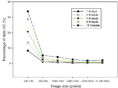
1) Multicore Performance: Table II summarizes the overall runtimes measured on the considered multicore platform while varying the number of utilized threads. By increasing the number of threads from 1 up to 16, the overall runtime decreases significantly from 2063.01 to 289.10 s for the largest image with a size of 11 500 4500 pixels. The data input and output (I/O) procedures were implemented on the basis of the Geospatial Data Abstraction Library (GDAL). These functions were implemented without parallelism either in the multicore version or in the GPU version, and therefore, the runtime of the I/O procedures remain constant under varying number of OpenMP threads. The data input takes 0.05–3.18 s for the six images with different sizes while the data output lasts between 0.09 and 2.52 s. The relative amounts of data I/O for the whole process are presented in Fig. 13. The figure enforces the observation that the relative amount of data I/O is, due to the high complexity in the calculation kernel, larger for small image sizes than for the bigger ones. With an increasing number of threads in the multicore parallel version, the serial I/O parts become relatively bigger and limit the overall speedup (Amdahl’s Law). The same holds true for the massively parallel GPU implementation. The overall speedup considering the data I/O of multicore acceleration is shown in Fig. 14, with the highest speedup of 4.58–7.14 for the different image sizes with up to 16 threads.

2) GPU Accelerator Performance: Table III summarizes the runtime results of the serial CPU version and GPU accelerated version. It should be noted that the overall runtime of the GPU acceleration is the sum of the runtime for the GPU driver start, data input, data transfer from host to device, calculation

Fig. 13. Percentage of the data input and output of the overall runtime.

Fig. 14. Overall speedup of the OpenMP-based multicore versions. on the GPU, data transfer from device back to host, and data output to the disc. Hence, the GPU accelerated version for the 500 100 image size takes 1.51 s and therefore almost as long as a serial CPU version with 1.74 s. Due to the nature of the architecture, the CPU version only includes the data input, calculation and data output procedures but no driver start and no additional data transfers. Even though the actual calculation on the GPU only takes about 0.03 s, the overall runtime including the mentioned overhead is a relatively long runtime of 1.51 s. With increasing the image size, the overhead becomes smaller and less significant compared to the kernel runtimes, whereby the GPU can play out its advantage in terms of highly parallel performance. For the largest image size, the GPU accelerated version takes 22.78 s to calculate the AOD on the GPU and 31.51 s in total while we measured 2063.01 s for the overall serial CPU implementation.

For illustrative purposes, Fig. 15 shows the percentages of the driver start, AOD calculation on the GPU, data transfer between host and GPU device and data I/O for different image sizes. As the data I/O, which takes 9.48%–18.08% of the overall runtime,

(9)

× TABLE III

RUNTIME OF THE SERIAL VERSION AND GPU ACCELERATION

Fig. 15. Summary plot describing the distributions of the overall runtime spend in the GPU device initialization, calculation in GPU, data transfer between host and GPU, and data I/O for the six image sizes.

is the same for all implementations, its runtime can be ignored when analyzing and comparing the parallel performance of the different implementations. Another common concern is that the data transfer time between the host and GPU device or its ratio to the overall program execution time can affect the parallel performance and might be one of the bottlenecks in GPGPU computing [8], [13], [33]. However, the data movement operations depicted in Fig. 15 only take 0.32%–5.19% of the overall runtime what corresponds to 5.91%–18.50% of the respective kernel calculation time. This indicates that most of the GPU processing time is spent in the most time-consuming computing operations and the data transfer to GPU memory is not the bottleneck for the proposed GPU implementation.

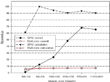
3) A Performance Comparison of Both Parallel Approaches: Comparing the parallel performances of both approaches, Fig. 16 shows the overall runtime for the serial version, the multicore implementation with up to 16 threads and the GPU accelerated version. The corresponding speedups of multicore and GPU versions are presented in Fig. 17. The best performance on the CPU, with a speedup of 7.x, is reasonably achieved when using as many threads as the physical cores

Fig. 16. Overall runtime comparison of the serial, the fastest multicore and the GPU accelerated versions.

Fig. 17. Overall and calculation speedup comparison between the fastest multicore and GPU accelerated version.

and it is relatively stable for different image sizes. The near linear speedup growth of the multicore version with increasing number of threads is depicted in Fig. 14, which indicates further enhancements for the multicore implementation in this paper for evolving multicore platforms with shared-memory parallelism that will assuredly emerge in the future.

As already stated, the overall speedup of the GPU version compared to the single core CPU one generally increases with enlarging the image size and achieves an overall speedup of 65.x for the image with 11 500 4500 pixels, while the multicore version is seven times faster than the serial one. The GPU therefore outperforms the fastest CPU version by a factor of 9. The pure calculation speedup of the GPU implementation compared to a single CPU core of 61.x–100.x is explicitly shown in Fig. 17. These measurements support the thesis that even near real-time quantitative retrieval could be achieved for smaller image sizes due to the massively parallel processing power offered by GPUs.

(10)

×

∼

Fig. 17 presents different calculation speedup trends along with the six image sizes for the OpenMP multicore and GPU implementations. While the speedups of both versions’ calculation kernels are relatively stable for the larger images, the GPU’s overall speedup increases among almost the whole range of image sizes. This is based on the decreasing relevance of other overheads such as the driver start and data transfer between the host and GPU device. Consequently, the GPU’s overall speedup is expected to remain relatively stable as soon as those overheads become negligible compared to the pure calculation time. As the multicore versions do not contain such overheads, their total speedups also remain relatively stable for the larger images. While the GPU can play out its parallel potential especially for larger images, Fig. 16 also shows that, for very small inputs, the overhead of using the GPU due to data transfers and driver start can be large enough to make the CPU performing better concerning the overall runtime even though the GPU kernel is by far faster than the one running on the CPU.

E. Energy Consumption and Code Migration Considerations Given that the energy consumption is a great concern in mis- sions, the power intakes of the different implementations for the largest image (11 500 4500 pixels) were measured using the power consumption meter Christ CLM1000 Professional (Plus) tracking data once per second. As the overall power can be divided into the dynamic power and static power [34], the difference P diff between the idle and load conditions is presented in Fig. 18 to evaluate the power we measured for the multicore and GPU accelerated implementations. For all measurements, we excluded the CPU’s and the main system’s idle power in the statistics, as it is present and identical for both the multicore and GPU accelerated implementations. However, the GPUs idle power intake is included in the GPU statistics as it is only presented in the GPU node. For the multicore implementation, the maximum recorded powers for 1, 2, 4, 8, and 16 threads are 35.7, 54.8, 67.9, 93.5, and 138.7 W, respectively, however, with significantly decreasing runtime when more threads are served. The average power intake of the GPU is 80 W and therefore in a range comparable to the eight threads version on the CPU, respectively, one CPU socket working with full capacity. It is important to note that the GPU, due to the algorithmic properties and our implementation, is by far not consuming its peak power intake ( 220 W).

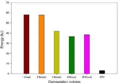
The overall energy consumptions are calculated as the sum of all power intake values per second, what is a reasonably good approximation of the actual energy expended. The results are presented in Fig. 19. The derived overall energy consumptions of the CPU version running on 1, 2, 4, 8, and 16 threads are 58.09, 57.84, 41.98, 36.74, and 38.39 kJ, while the GPU implementation consumes only 3.15 kJ. The multicore implementation has a principally decreasing consumption trend with the processors increasing. The GPU implementation consumes only 8.57% of the one serving eight threads, which is the most energy efficient multicore implementation. When increasing the number of threads from 8 to 16 for the multicore implementation, the results show that even though the runtime of

Fig. 18. Power intake curves of the multicore and GPU implementations.

Fig. 19. Overall energy consumption comparison of the multicore and GPU implementations.

the method decreases significantly, the actual intake of power increases significantly because configuring the OpenMP environment to 16 instead of 8 threads enables the utilization of both available sockets instead of only one. The overall consumed energy for 16 threads is slightly higher than that for 8 threads while the runtime is by far smaller with 16 threads, as the usage of a second CPU adds a further notably energy overhead. This also shows that in case of considering purely the energy efficiency, not the fastest performing 16 threads version but the 8 threads version would be the implementation of choice.

Considering the application and available environments in this paper, the GPU accelerator has demonstrated advantages in both parallel performance and energy efficiency. This result is of course specifically related to the fact that the investigated application fits well to a GPUs parallel architecture’s properties. GPUs are generally considered to be extremely high energy consuming and thus not suitable for on-board processing mis- sions. Multicore architectures on the other hand are evolving very quickly and, therefore, are expected to offer alternatives

(11)

with more tolerable radiation and energy consumption requirements [9], [15]. These results show that at least concerning the energy consumption and performance, using GPUs would be the best choice for this application.

Easy programmability is also an important evaluation cri- terion in making use of HPC architectures in remote sensing applications and it is undoubtedly easier and more conve- nient for geoscientists to migrate algorithms and codes toward a multicore implementation using OpenMP rather than GPU CUDA-C codes.

IV. CONCLUSION AND FUTURE RESEARCH PERSPECTIVES

In this work, two implementations of an AOD quantitative retrieval algorithm SRAP-MODIS from MODIS satellite data have been developed on multicore processors and a GPU platform. The multicore implementation provides a nearly 7.x overall speedup for image analysis scenarios, which is considered reasonable. The GPU implementation offers a maximum

100.x calculation speedup and 68.x overall speedup including the procedures data I/O and data transfer for the prepared six image datasets. For smaller image size scenarios, near real-time retrieval based on the GPU implementation could be achieved. The experimental results in this paper indicate that further applications which call for fast response of AOD retrieval such as the monitoring of volcanic eruptions or forest fires, air quality, and fast atmospheric correction could benefit from the development of efficient parallel implementations of AOD retrieval. Our work also provides implementation pattern suggestions for similar quantitative remote sensing retrieval applications performing calculations with a pixel-based nature. The comparison from the perspectives of the parallel performance, energy efficiency and code migration considerations in this work is intended to give actual suggestions for geoscientists with different computational requirements.

Despite the promising results reported in this paper, better understandings of the overall quantitative remote sensing chain which also includes the time-consuming preprocessing geometric correction and other procedures such as the image cut, image resize, and cloud mask are needed. There are also non pixel-based operations like the spatial neighborhood-based operations and spectral domain operations which need compre- hensive parallel pattern designs and implementations for both multicore and GPU computing platforms to achieve the best performance. Considering the speedups observed in this paper gained from the multicore and GPU implementations, we will accomplish a heterogeneous solution for the parallel retrieval using the two platforms cooperatively.

ACKNOWLEDGMENT

The authors would like to thank Fraunhofer Institute for Algorithms and Scientific Computing SCAI for the multicore and GPU platform used in this paper. They would also like to thank the anonymous reviewers for their constructive comments and suggestions on this paper. MODIS data were available through NASA MODIS LAADS.

REFERENCES

[1] A. Plaza, Q. Du, Y.-L. Chang, and R. L. King, “High performance com-

puting for hyperspectral remote sensing,” IEEE J. Sel. Topics Appl. Earth

Observ. Remote Sens., vol. 4, no. 3, pp. 528–544, Sep. 2011.

[2] E. Masuoka, C. Tilmes, N. Devine, G. Ye, and M. Tilmes, “Evolution of

the MODIS science data processing system,” in Proc. IEEE Int. Geosci.

Remote Sens. Symp., 2001, pp. 1454–1457.

[3] Y. Xue, X. He, H. Xu, J. Guang, J. Guo, and L. Mei, “China Collection

2.0: The aerosol optical depth dataset from the synergetic retrieval of aerosol properties algorithm,” Atmos. Environ., vol. 95, pp. 45–58, 2014.

[4] C. A. Lee, S. D. Gasster, A. Plaza, C.-I. Chang, and B. Huang, “Recent

developments in high performance computing for remote sensing: A review,” IEEE J. Sel. Topics Appl. Earth Observ. Remote Sens., vol. 4, no. 3, pp. 508–527, Sep. 2011.

[5] Y. Xue et al., “A high throughput geocomputing system for remote sens-

ing quantitative retrieval and a case study,” Int. J. Appl. Earth Observ. Geoinf., vol. 13, pp. 902–911, 2011.

[6] Y. Xue et al., “Grid-enabled high-performance quantitative aerosol

retrieval from remotely sensed data,” Comput. Geosci., vol. 37, pp. 202–

206, 2011.

[7] W. Guo, J. Gong, W. Jiang, Y. Liu, and B. She, “OpenRS-Cloud: A

remote sensing image processing platform based on cloud computing environment,” Sci. China Technol. Sci., vol. 53, pp. 221–230, 2010.

[8] C. Gonzalez, S. Sánchez, A. Paz, J. Resano, D. Mozos, and A. Plaza, “Use

of FPGA or GPU-based architectures for remotely sensed hyperspectral image processing,” Integr. VLSI J., vol. 46, pp. 89–103, 2013.

[9] S. Bernabe, S. Sanchez, A. Plaza, S. López, J. A. Benediktsson, and R. Sarmiento, “Hyperspectral unmixing on GPUs and multi-core processors: A comparison,” IEEE J. Sel. Topics Appl. Earth Observ. Remote Sens., vol. 6, no. 3, pp. 1386–1398, Jun. 2013.

[10] E. Torti, M. Acquistapace, G. Danese, F. Leporati, and A. Plaza, “Real-

time identification of hyperspectral subspaces,” IEEE J. Sel. Topics Appl.

Earth Observ. Remote Sens., vol. 7, no. 6, pp. 2680–2687, Jun. 2014.

[11] J. M. Molero, E. M. Garzón, I. Garcıa, E. S. Quintana-Ortı, and A. Plaza,

“Efficient implementation of hyperspectral anomaly detection techniques on GPUs and multicore processors,” IEEE J. Sel. Topics Appl. Earth Observ. Remote Sens., vol. 7, no. 6, pp. 2256–2266, Jun. 2014.

[12] D. S. Efremenko, D. G. Loyola, A. Doicu, and R. J. Spurr, “Multi-core- CPU and GPU-accelerated radiative transfer models based on the discrete ordinate method,” Comput. Phys. Commun., vol. 185, pp. 3079–3089, 2014.

[13] X. Su, J. Wu, B. Huang, and Z. Wu, “GPU-accelerated computation for

electromagnetic scattering of a double-layer vegetation model,” IEEE J.

Sel. Topics Appl. Earth Observ. Remote Sens., vol. 6, no. 4, pp. 1799– 1806, Aug. 2013.

[14] J. Mielikainen, B. Huang, and H. Huang, “GPU-accelerated multi-profile

radiative transfer model for the infrared atmospheric sounding interferometer,” IEEE J. Sel. Topics Appl. Earth Observ. Remote Sens., vol. 4, no. 3, pp. 691–700, Sep. 2011.

[15] A. Remón, S. Sánchez, S. Bernabé, E. S. Quintana-Ortí, and A. Plaza,

“Performance versus energy consumption of hyperspectral unmixing

algorithms on multi-core platforms,” EURASIP J. Adv. Signal Process.,

vol. 2013, pp. 1–15, 2013.

[16] Y. J. Kaufman and D. Tanré, “Strategy for direct and indirect methods for

correcting the aerosol effect on remote sensing: From AVHRR to EOS- MODIS,” Remote Sens. Environ., vol. 55, pp. 65–79, 1996.

[17] L. Mei et al., “Integration of remote sensing data and surface observations to estimate the impact of the Russian wildfires over Europe and Asia during August 2010,” Biogeosciences, vol. 8, pp. 3771–3791, 2011.

[18] M. Lin et al., “Regression analyses between recent air quality and visi-

bility changes in megacities at four haze regions in China,” Aerosol Air Qual. Res., vol. 12, pp. 1049–1061, 2012.

[19] A. T. Evan, J. P. Kossin, and V. Ramanathan, “Arabian Sea tropical cyclones intensified by emissions of black carbon and other aerosols,”

Nature, vol. 479, pp. 94–97, 2011.

[20] T. Stocker et al., IPCC, 2013: Climate Change 2013: The Physical

Science Basis. Contribution of Working Group I to the Fifth Assessment Report of the Intergovernmental Panel on Climate Change. Cambridge, U.K.: Cambridge Univ. Press, 2013.

[21] L. Mei et al., “Validation and analysis of aerosol optical thickness retrieval over land,” Int. J. Remote Sens., vol. 33, pp. 781–803, 2012. [22] Y. Xue and A. Cracknell, “Operational bi-angle approach to retrieve

the Earth surface albedo from AVHRR data in the visible band,” Int. J.

(12)

[23] J. Tang, Y. Xue, T. Yu, and Y. Guan, “Aerosol optical thickness determi-

nation by exploiting the synergy of TERRA and AQUA MODIS,” Remote

Sens. Environ., vol. 94, pp. 327–334, 2005.

[24] NASA Goddard Space Flight Center, Level 1 and Atmosphere Archive

and Distribution System [Online]. Available: http://ladsweb.nascom.nasa. gov/data/search.html, accessed on 2013.

[25] E. Ayguadé et al., “The design of OpenMP tasks,” IEEE Trans. Parallel

Distrib. Syst., vol. 20, no. 3, pp. 404–418, Mar. 2009.

[26] E. Christophe, J. Michel, and J. Inglada, “Remote sensing processing:

From multicore to GPU,” IEEE J. Sel. Topics Appl. Earth Observ. Remote

Sens., vol. 4, no. 3, pp. 643–652, Sep. 2011.

[27] K. Karimi, N. G. Dickson, and F. Hamze, “A performance comparison of

CUDA and OpenCL,” arXiv: 1005.2581, 2010.

[28] INTEL. (2012). Intel ® Xeon ® Processor E5-2600 Series [Online].

Available: http://download.intel.com/support/processors/xeon/sb/xeon_ E5-2600.pdf, accessed on 2014.

[29] B. P. Flannery, W. H. Press, S. A. Teukolsky, and W. Vetterling,

Numerical Recipes in C. Cambridge, U.K.: Univ. Cambridge, 1992.

[30] S. Bell, A Beginner’s Guide to Uncertainty of Measurement. Middlesex,

U.K.: National Physical Lab., 2001.

[31] R. Levy et al., “The Collection 6 MODIS aerosol products over land and

ocean,” Atmos. Meas. Techn., vol. 6, pp. 2989–3034, 2013.

[32] A. Kokhanovsky et al., “The inter-comparison of major satellite aerosol

retrieval algorithms using simulated intensity and polarization charac- teristics of reflected light,” Atmos. Meas. Techn., vol. 3, pp. 909–932, 2010.

[33] M. Abouali, J. Timmermans, J. E. Castillo, and B. Z. Su, “A high per-

formance GPU implementation of surface energy balance system (SEBS)

based on CUDA-C,” Environ. Modell. Softw., vol. 41, pp. 134–138, 2013.

[34] S. Hong and H. Kim, “An integrated GPU power and performance model,” in Proc. ACM SIGARCH Comput. Archit. News, 2010, pp. 280– 289.

[35] J. Nickolls and W. J. Dally, “The GPU computing era,” IEEE Micro, vol. 30, no. 2, pp. 56–69, Mar./Apr. 2010.