Sparse Generalised Principal Component Analysis
Luke Smallmana,∗, Andreas Artemioua, Jennifer Morgana aCardiff University, School of Mathematics, Senghennydd Road, Cardiff, CF24 4AG
Abstract
In this paper, we develop a sparse method for unsupervised dimension reduction for data from an exponential-family distribution. Our idea extends previous work on Generalised Principal Component Analysis by addingL1 and SCAD penalties to introduce sparsity.
We demonstrate the significance and advantages of our method with synthetic and real data examples. We focus on the application to text data which is high-dimensional and non-Gaussian by nature and discuss the potential advantages of our methodology in achieving dimension reduction.
Keywords: dimension reduction, PCA, text mining, exponential family
2010 MSC: 62H25, 62-09, 62J07, 68T50
1. Introduction
Dimension reduction tools are now a common-place solution to two of the major dif-ficulties incurred by high-dimensional big data: computational expense and a breakdown of classical statistical methodology. The former stems from both the difficulty of storage and access of huge datasets, especially when they are not sparse, and from the time costs of running many popular algorithms on such data. The latter arises as most classical methodology for inference was introduced for low-dimensional data, and often cannot generalise beyond a few dimensions. As such, dimension reduction techniques are used to extract a lower-dimensional manifold which describes the structure of the original data as well as possible. Dimension reduction methodology can be broadly split into two categories: methods for feature selection and methods for feature extraction. The for-mer chooses a subset of the original features, whilst the latter finds a (low-dimensional) vector-valued function of the original features. Many examples of feature extraction are referred to as “linear”, as the extracted features are simply a linear combination of the original features. In this paper, we will combine two well-known feature selection tech-niques with a generalised principal component analysis algorithm (a well-known feature extraction method) to achieve sparse dimension reduction for non-Gaussian data. We will focus on the application of this method to Poisson-distributed data, which has re-ceived increased attention lately due to the application of Poisson-based techniques in the analysis of text data. PCA (and the variants thereof which we will discuss in this
∗Corresponding author
Email address: [email protected](Luke Smallman)
article) are methods for unsupervised dimension reduction. That is, they do not require or use any response associated with the data which may be available, in contrast to supervised methods which do require response information and make use of it to inform the dimension reduction.
Principal Component Analysis (PCA) has been extensively used in the literature since its introduction by Pearson (1901) and more importantly by Hotelling (1933). It has mainly been used for dimension reduction through feature extraction. The main objective of PCA is to sequentially extract orthogonal features which maximize the vari-ability of our data. One of PCA’s most useful features is that it produces a linear transformation of the data, calculated with a simple matrix multiplication. This is very advantageous for dimension reduction scenarios, when calculating a complicated function of the entire dataset would be infeasibly expensive in computation time. Instead, the loadings matrix (the matrix which performs the dimension reduction) can be calculated using a smaller, representative dataset, and then the transformation quickly calculated for the rest of the data. PCA was introduced for Gaussian distributed data and has been extended significantly over the years to address different research problems (see for example Tipping and Bishop (1999), Collins et al. (2002), Ding and He (2004), de Leeuw (2006) and Diederichs et al. (2013) among others). The need to develop a generalised version of PCA to address application to the exponential family of distributions (which encompasses a wide variety of models for real-world data) was recognised in Landgraf and Lee (2015) who developed Generalised Principal Component Analysis (GPCA).
In this work, we focus on the application of PCA algorithms to text data which is naturally high-dimensional and non-Gaussian. Text data is usually transformed into numerical data so that classical statistical tools can be applied to it. One of the more common ways to do so is to construct a “document-term matrix” where each row is an observation and each unique word/term within the collection is a column. Then the ijth entry is an integer denoting the number of times theith document contains thejth
term. This is an inherently high-dimensional representation, and the number of terms ptypically grows with the number of documents n. However, we expect that many of these terms will be uninformative for many purposes. In general, given a wide variety of documents we often expect that there will be a significant number of terms which are introduced solely because of the form of the writing and which will be common across a number of the documents, even if they are very different in content. For instance, in a collection of letters we would expect to find salutations, well-wishings, addresses, from-lines and the like; such inclusions would likely be common across most letters but would be unlikely to convey any meaning of interest to the text miner. Further, grammar and structure of language dictates many words, such as pronouns, “and”, “the”, etc., which are important to a human reader but not to a computer. These all expand the dimension of the dataset. Hence, we would like to apply some method of dimension reduction which can provide a much smaller representation of the data. We also desire that our transformed representation does not use terms which do not provide any useful meaning (such as “and”, “Yours sincerely”). In order to achieve this, we will require our transformation to have sparse loadings; including a term must improve the model more than some penalty. This also has the advantage of increasing the interpretability of our loadings. Without sparsity, most loading components are typically non-zero; with sparsity, we can often reduce the number of non-zero components to a manageable number to inspect. In the context of text data, this means we can find a list of which
terms are considered important for understanding a document. To apply GPCA and our extension, we require an exponential family model for the data. Given the form of the document-term matrix as a count of term occurrences, we prescribe a simple model for the data where the number of occurrences of termj across each document is given by a Poisson distribution with some meanλj.
In Section 2 we will discuss previous work, focusing on extensions to PCA and meth-ods for dimension reduction of text data. In Section 3 we will define GPCA. We will then extend this to Sparse Generalised Principal Component Analysis (SGPCA) in Section 4.1, and present an efficient way to estimate it. We will compare their performances on both synthetic datasets and two healthcare datasets in Section 5 and Section 6 respec-tively, before discussing the implications of this work and plans for future work in Section 7. To improve readability, detailed derivations will be relegated to the appendices.
2. Previous Work
In this section, we will discuss some related previous work, focusing both on extensions to the usual Gaussian PCA and on dimension reduction methods for text data.
2.1. PCA Extensions
We begin in this section by discussing PCA extensions, first defining Gaussian PCA, then Sparse PCA, Joint Sparse PCA and Robust PCA.
2.1.1. PCA Summary
LetX∈Rn×pbe a data matrix formed of nobservations of ap-dimensional random variable X, that is X = [x1|x2| · · · |xn]T with xi = (xi1, . . . , xip)T for i = 1, . . . , n. Then the usual definition of (Gaussian) PCA is the (k-dimensional) orthogonal linear projection such that the first component of the projected data is in the direction with the most variance, the second component is in the direction with the second most variance, and so on. It is also well-established in the literature that the PCA approximation toX minimises the squared reconstruction error (the difference between the lower-rank approximation toX and the trueX).
2.1.2. Sparse PCA
Sparse PCA (SPCA) from Zou et al. (2006) is based around their “SPCA criterion” which finds an approximation toXof the formXBAT(A,B∈Rp×k) which minimises
kX−XBATk22+λ k X i=1 kβik22+ k X j=1 λ1,jkβjk1,
subject toATA = Ik and whereB = [β1, . . . ,βk]. In this case, the matrix Bgives the loadings, and has both L1 and L2 penalties imposed on its entries, inducing sparsity.
The combination of these penalties is often known as the elastic net (due to Zou and Hastie (2005)).
2.1.3. Sparse PCA via Rotation and Truncation
This method, developed in Hu et al. (2016), provides an alternative method for sparse PCA to that of Zou et al. (2006). The essential idea is that any rotation of the PCA loadings provides an orthogonal basis spanning the same subspace. Thus, the authors propose a method to find a rotation matrix and a sparse basis which approximates the PCA loadings after rotation. They offer four methods of truncation, which is used to find the approximating sparse basis, each of which offers slightly different performance and control.
2.1.4. Robust PCA
In Kwak (2008), Kwak formulated Robust PCA (RPCA) in terms of the projection variance maximisation formulation of PCA. That is, viewing PCA as finding the projec-tion matrixU∈Rp×k which maximisesTr UTCU
subject toUTU = I
k, whereCis the covariance matrix ofX. This problem can be reformulated as maximisingPn
i=1kU Tx
ik22
subject to the same orthogonality constraint. They propose modifying the norm used in this formulation to yield the problem of maximisingPn
i=1kU Tx
ik1subject toUTU = Ik.
This increases the robustness of the problem to outliers.
2.1.5. Sparse Probabilistic Principal Component Analysis
Sparse Probabilistic Principal Component Analysis (SPPCA), formulated in Guan and Dy (2009) is an extension of Probabilistic PCA (Tipping and Bishop (1999)) and SPCA (Zou et al. (2006)), essentially working to combine the two. They specify a probabilistic model for PCA which incorporates a sparsity inducing prior on the loadings. In the paper they investigate three different priors: a Laplacian prior, an inverse-Gaussian prior and a Jeffrey’s prior. In this work we consider the Laplacian prior case which corresponds to anL1penalty on the components.
2.1.6. Sparse Exponential Family Principal Component Analysis
Lu et al. (2016) proposed Sparse Exponential Family Principal Component Analysis (SEPCA) roughly as an extension to SPCA (Zou et al. (2006)) to the exponential family. Given dataX, their problem is specified by
min Z:ZTZ=I,W,b X n A WTzn+b −TrZW +1bTXT+P(W,b)
whereAis a function specified by the exponential distribution andP(·,·)is a sparsifying penalty. In particular, P(W,b) =λ0 ZW +1b T 2 2+ k X i=1 λi|Wi|
which the authors claim enables reconstruction of the principal components in degenerate cases and induces sparsity in the loading vectors.
2.2. Text Data Dimension Reduction Methods
In this section we will briefly discuss three methods for text dimension reduction: Multinomial Inverse Regression, Nonnegative Matrix Factorisation and Latent Dirichlet Allocation.
2.2.1. Multinomial Inverse Regression
Multinomial Inverse Regression (MNIR), introduced in Taddy (2013) and further in Taddy (2015), is a dimension reduction method for text data based around a multinomial model for text data. The method is supervised, intended to provide a reduced dimension projection of the data suitable for use in a classification algorithm or similar. As such, it requires a response variable for each observation, which it uses to determine informative terms. As such, our comparison with it will only be performed for the classed synthetic dataset in Section 5.2. We will not include it in our comparison on the healthcare dataset in Section 6, as it is only capable of producing a projection of the same dimension as the response variable; as our response in this case is univariate, but all the other methods will be used to provide a3-dimensional representation.
2.2.2. Nonnegative Matrix Factorisation
Nonnegative Matrix Factorisations (for an overview, see Gillis (2014)) aims to fac-torise a nonnegative matrix X in the form X = WH, where W and H are both also nonnegative. In the framework of text mining, the basis vectors formed by W can be interpreted as topics in term-space andHcan be interpreted as giving the importance of each topic for each document.
2.2.3. Latent Dirichlet Allocation
Latent Dirichlet Allocation, from Blei et al. (2003), is a (generative) probabilistic model for text. Roughly, it assumes each document draws a vector of topic probabilities, then repeatedly draws a topic according to those probabilities, drawing a word each time it draws a topic. For full details of how these quantities are distributed (and how the underlying probabilities are estimated), consult Blei et al. (2003), but for our purposes the most important aspect of the model is that it is used to estimate a matrix
B = [β1|. . .|βk]T, where each vectorβigives (multinomial) probabilities of drawing each of the words in the vocabulary given that the word is drawn according to topici. It is important to note that the choice of the word “topics” is to assist interpretation; this method is not supervised, the topics are driven only by the observed word counts and the number of topics is a user-chosen parameter.
3. Generalised PCA
In this section, we introduce the Generalised PCA of Landgraf and Lee (2015) for exponential family distributions; for completeness and clarity, we begin by discussing exponential families and some of their properties.
3.1. Exponential Family Distributions
Let X ∈ Rp be a random vector from a distribution in the exponential family of distributions with parameter θ. The probability density function for x has the form f(x|θ) =h(x) exp xTθ−b(θ)
, whereh(x)andb(θ)are both scalar-valued functions, with the former serving to normalise the distribution. A straightforward calculation shows thatE(X) =b0(θ). Thecanonical link function g is defined as the left inverse of b0, i.e. g(b0(θ)) =θ. The model where the expected value is set to the observed data is known as thesaturated model, its parameters will be denoted byθ, and it will be equal˜ tog(x).
3.2. GPCA Definition
In Section 2.1.1 we gave the usual formulation of PCA. An equivalent formulation of PCA, suitable for the definition of GPCA, is to find the optimum U ∈ Rp×k and µ= (µ1, . . . , µp)T∈Rp which minimise n X i=1 xi−µ−UUT(xi−µ) 2 2,
whereUis the projection matrix. With a Gaussian distribution (with known variance), the canonical link function is the identity function, so the saturated model parameters are the data themselves, the natural parameter is the mean and the deviance is propor-tional to squared error loss. We can see then that, under the assumption of a Gaussian distribution, the above formulation of PCA is equivalent to finding the deviance-optimal approximation to the natural parameters of the form µ+ UUTθi˜ −µ. This can be
readily extended to any exponential family distribution; we find that the deviance has the following form (details of the derivation can be found in Appendix A1):
D(U,µ) = n X i=1 p X j=1 ( bj µj+ h UUTθi˜ −µi j −xij µj+ h UUTθ˜i−µ i j ) =X i,j Dij (1)
where thebj functions are subscripted to allow for the possibility of each component of our random vector coming from a different exponential family distribution (although we will proceed to examine only cases where all variables are from the same distribution, albeit with different natural parameters). We denote the coordinate-observation-wise devianceDij and low-rank natural parameter estimate θij, defined by
Dij =bj(θij)−xijθij, θij =µj+
h
UUTnθi˜ −µoi j
Thus we can now define the GPCA of Landgraf and Lee (2015) as the projection given by theUthat minimises the deviance. Formally, let
U∗,µ∗= arg min U∈Rp×k,µ∈Rp
D(U,µ),
then g(X)−1(µ∗)T
U∗ is the GPCA projection.
4. Sparse GPCA
In this section we will present the definition of SGPCA and an algorithm for approx-imating it.
4.1. Definition
There is a wide literature using penalties on regression coefficients to induce sparsity in statistical procedures, primarily focusing on theL1(LASSO-type penalty, see Tibshirani
(1996)) andL2 (ridge-type penalty, see Hoerl and Kennard (1970)) penalties as well as
combination of the two (elastic net, see Zou and Hastie (2005)). Another popular penalty with desirable features is the Smoothly Clipped Absolute Deviation (SCAD) penalty of Fan and Li (2001). The SCAD penalty is usually defined by its derivative
PS0(θ;λ, a) =λI(θ≤λ) +(aλ−θ)+
a−1 I(θ > λ) (2)
wherex+= max (x,0). The penalty has two parameters,λanda. The former is usually
chosen on a problem-by-problem basis, often with some form of cross-validation, while the latter is often taken as3.7due to an argument in Fan and Li (2001). Integrating, as in Appendix A4, shows that the penalty has the form
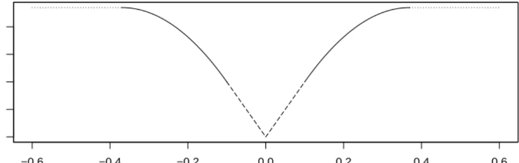
PS(θ;λ, a) = λθ 0< θ≤λ −θ2−2aλθ+λ2 2(a−1) λ < θ≤aλ (a+1)λ2 2 aλ < θ (3)
That is, “near” 0the penalty is linear and decreases towards the origin, “far” from0 the penalty is a positive constant, and between the two areas the penalty is quadratic, again decreasing towards the origin. This can also be seen in Figure 4.1a, where the linear section is dashed, the constant section is dotted, and the quadratic section is solid. Note that the figure shows the symmetrised SCAD penalty (that is, it shows the penalty on |θ|). In Figure 4.1b we also show the penalty for three different values ofλ(while holding afixed at 3.7) to demonstrate the behaviour of the penalty asλchanges.
In contrast, the L1 penalty is much simpler, being only the absolute value of the
component. Clearly, the L1 penalty differs only by a multiplicative factor from the
SCAD penalty near0, but unlike the SCAD penalty it does not change in form across its domain. From a computational point of view, this means that theL1 penalty is slightly
less computationally expensive, not requiring the evaluation of any conditional operators. Although the evaluation of these operators is not particularly expensive, the estimation algorithm we will discuss later requires very frequent evaluation of the penalty function. The motivation behind theL1penalty is to ensure that non-zero coefficients will only be added to the model if they reduce the unpenalised objective function by an amount proportional to their magnitude. “Large” coefficients therefore can be interpreted as coefficients which make the model significantly better. In our method,λLis the coefficient of proportionality which determines how much a unit increase in a coefficients distance from 0 must decrease the objective function for it to be a permissible change. The SCAD penalty performs a similar function to theL1 penalty; the primary difference is
that once a coefficient is sufficiently large in absolute value, the penalty does not increase (i.e. the linear region in Figure 4.1a). Ideally, this should ensure that once a coefficient is determined to be significant, its magnitude is decided by the objective function without the penalty function artificially reducing it.
For this particular problem, we would like to penalise only U by imposing upon it either anL1penalty, the SCAD penalty, or a combination of both. Specifically, we define
(a) The (symmetrised) SCAD penalty, withλ= 0.1anda= 3.7 −0.6 −0.4 −0.2 0.0 0.2 0.4 0.6 0.000 0.010 0.020 θ
(b) The (symmetrised) SCAD penalty for λ = 0.1 (solid), λ = 0.15 (dashed), and λ = 0.2 (dotted) −1.0 −0.5 0.0 0.5 1.0 0.00 0.04 0.08 θ
the penalty function
P(U, λL, λ, a, λS) =
X
i,j
{λL|Uij|+λSPS(|Uij|;λ, a)} (4)
The coefficientλS ≥0of the SCAD penalty, like λL, is used to control the weighting of SCAD against theL1 penalty and the deviance. We introduce this, as whilst changing λchanges the magnitude of the SCAD penalty, it also changes the characteristics signif-icantly by changing the knots of the quadratic splines. Notice that we place the SCAD penalty on the absolute value of each component, not on the value itself, as the SCAD penalty is only defined for positive values. We do not penaliseµas we desire it to capture (in some sense) the mean of each of the component natural parameters. Non-zero entries in µ are to be expected, and allow us to centre the natural parameters. We can now define our SGPCA objective function
S(U,µ;λL, λ, a, λS)..=D(U,µ) +P(U;λL, λ, a, λS) (5) For the remainder of this paper, we will not explicitly notate the dependence onλL, λS, orain order to simplify notation.
Remark 1. Here we emphasize that in this problem it does not make sense to apply an L2penalty toU, since the usual definition of theL2penalty for matrices (also known as the Frobenius norm) is equivalent toTr UTUwhich, by the semi-orthogonality ofU, is
Tr (Ip) =p. Consequently, for the purposes of this article we use only theL1 and SCAD penalties imposed onU. Other penalties will be explored in the future.
Remark 2. In the rest of this article we will consider three SGPCA formulations: the L1penalty, the SCAD penalty and a linear combination. We have no a priori reason to believe that the combined penalty ought to be superior to either, but our specification of the problem lends itself well to considering it; as such it would be remiss not to investigate its performance.
4.2. Estimation Algorithm
In general, (5) is non-convex inUandµ. This, combined with the non-differentiability of the penalty function at0and the semi-orthogonality constraint uponU, make finding the optimum values ofU andµdifficult. One way to deal with the semi-orthogonality condition would be to use a Lagrangian method; in Appendix A2 we use a Lagrange mul-tiplier augmented objective function to derive first order optimality conditions. However, the Lagrangian still has the difficulties of non-differentiability. Instead, in Section 4.2.1 we will derive a perturbed majoriser of the objective function to be used in a Majorise-Minimise (MM) algorithm using the results of Hunter and Li (2005). Crucially, this per-turbed majoriser will be differentiable, allowing us to use gradient-based optimisation. In Section 4.2.2, we will demonstrate the method of Wen and Yin (2013) to perform such optimisation whilst preserving the semi-orthogonality constraints.
4.2.1. Majorisation
The crux of our majorisation procedure is the method of Hunter and Li (2005), who developed theory for majorising penalty functions of the formP(θ) =Pp
i=1λipi(|θi|),
where the functions pi(·) are non-negative. Both the L1 and SCAD penalties can be written in this form, allowing us to use their majorisation procedure.
To illustrate, let us consider the ijth component of U. For notational simplicity, let
us denote this component byu. Then the contribution ofuto the penalty functionP(U)
isλL|u|+λSPS(|u|;λ, a)
The MM algorithm we will construct is iterative, so at time-steptwe have a previous value for each component, which we will denote u(t−1). We will first construct the majoriser and perturbed majoriser for theL1 penalty. We can approximate|u| by
|u| ≈ u (t−1) + u2− u(t−1)2 2u(t−1) (6)
In Hunter and Li (2005), the authors showed that this function majorises the exact componentL1penalty function, justifying its use in a majorisation of the entire objective
function. We can then construct the perturbed approximate L1 penalty function by
modifying the denominator
|u| ≈ u (t−1) + u2− u(t−1)2 2 ε+u(t−1) (7)
where ε > 0. This function is now well-defined for all values of u and u(t−1), and furthermore is differentiable in both too. It is clear that as ε ↓ 0 (where ↓ indicates approaching from above), this perturbed penalty tends to (6).
We now consider the case of the SCAD penalty (ignoring for now the multiplicative factorλS), which can be majorised using the formulation of Hunter and Li (2005) by
PS u (t−1) ;λ, a + u2− u(t−1)2PS0 u(t−1) +;λ, a 2u(t−1) (8)
where the +denotes the right-hand limit. The only pertinent case is when u(t−1)= 0,
in which case PS0(0+) = λ. As before, we construct the perturbed approximation by replacing the denominator
PS u (t−1) ;λ, a + u2− u(t−1)2PS0 u(t−1) +;λ, a 2 ε+u(t−1) (9)
Like before, (9) tends to (8) asε↓0. Consequently, we might expect that the optimum using (7) and (9) would be close to the optimum using (6) and (8) for sufficiently small ε, while allowing us to use gradient-based optimisation methods.
Remark 3. It is worth noting that neither (7) or (9) majorise the L1 penalty or the
SCAD penalty respectively. Instead, Hunter and Li (2005) show that they majorise a perturbed version of the respective penalties. The interested reader is referred to their paper for the details. From now, we will refer to them as majorisers, with the understanding that this only holds exactly in the limit asε↓0.
In the original formulation of GPCA, the authors use a quadratic approximation to the deviance which they then majorise in order to construct an MM algorithm for their problem. The particular majorisation they use allows them to find a closed form minimiser overµand reduces to an orthogonal Procrustes problem inUfor each iteration (for more details on the orthogonal Procrustes problem, see Schönemann (1966)). The introduction of the penalty term we use does not allow the use of the same technique here. Instead, we majorise only the penalty term, leaving the deviance unchanged. This gives us our majorised objective function:
MU,µ U (t−1)..=D(U,µ) +Mε P U U (t−1) (10) whereMε
P is the perturbed majoriser of the combinedL
1and SCAD penalties, given by:
MPε U U (t−1)= n X i=1 p X j=1 ( λL U (t−1) ij +λSPS U (t−1) ij ;λ, a + U2 ij− U(ijt−1) 2 λL+λSPS0 U (t−1) ij +;λ, a 2ε+ U (t−1) ij ) (11) 4.2.2. Gradient-Based Optimisation
In Wen and Yin (2013), the authors derive a method for gradient-based optimisation which preserves orthogonality. Their scheme works in generality, for all differentiable optimisation problems with orthogonality constraints, but we will illustrate it only in application to solving our perturbed majoriser problem.
Given a current estimate of U (denoted U(t−1)) and the gradient of the objective function at that point (denoted G), we construct the skew-symmetric matrix A ..= G U(t−1)T
−U(t−1)GT. Wen and Yin showed that the function Y(τ)..=I +τ 2A −1 I−τ 2A U(t−1)
defines a descent direction forτ ≥0. Additionally,Y(τ)is smooth inτandY(τ)TY(τ) = U(t−1)TU(t−1) = I, so each value of τ produces a feasible point preserving the semi-orthogonality condition onU. Minimisation then proceeds by line search along{Y(τ)}τ≥0.
We use a standard line search algorithm given in Nocedal and Wright (2006) and recommended in Wen and Yin (2013). The details of this method are omitted, as any one-dimensional optimisation method would suffice, but the interested reader is referred to both sources. We also perform a gradient-based algorithm to find optimal values of
µ; as there are no constraints on µto deal with, any standard optimisation procedure
can be used.
The required gradients are given as follows, their derivation can be found in Appendix
A3: ∂M ∂Urs = n X i=1 p X j=1 ( b0j µj+ h UUTθi˜ −µi j −xij ×δrjUT[s] ˜ θi−µ +Ujs ˜ θir−µr ) + λL+λSPS0 U (t−1) rs +;λ, a Urs ε+ U (t−1) rs (12) ∂M ∂µr = n X i=1 p X j=1 b0j µj+ h UUTθ˜i−µ i j −xij δjr− UUT jr (13) 4.2.3. Implementation
Code to calculate the optimal values ofµandUwas written in R (R Foundation for Statistical Computing, Vienna (2011)). We alternated between optimising overµusing the R built-inoptim function and optimising over U using our own implementation of the gradient-based method of Wen and Yin (2013), stopping when the objective function changed between iterations by less than a given tolerance, which we selected on a case-by-case basis. Our majorisation-based method requires that we have an initial estimate forµ and U. As the gradient-based optimisation method for U preserves the value of
UTU, we also require that our initial estimate for U is left semi-orthogonal. To that end, we follow the same procedure as for GPCA in settingµ(0)= ColMeans (g(X))and U(0) = EigVec
l
g(X)−1 µ(0)T
(i.e. the first l eigenvectors, ordered in decreasing eigenvalue magnitude).
4.2.4. Estimation procedure
To summarise, estimation proceeds as follows: • Step 1:
1. CalculateΘ˜ ..=g(X)
2. Setµ(0) to the column means ofΘ˜
3. SetU(0) to the firstleigenvectors ofΘ˜−
1 µ(0)T
• Step 2: to be repeated fort= 1,2, . . .
1. Letµ(t)be the minimiser of (10) with respect toµ, lettingUin (10) beU(t−1)
calculated usingoptim) with gradient given by (13)
2. (a) Calculate the gradientGof (10) with respect toUevaluated atU(t−1),µ(t) using (12) (b) SetA..= G U(t−1)T −U(t−1)GT (c) DefineY(τ)..= I +τ 2A −1 I−τ 2A U(t−1)
(d) Findτ∗≥0 which minimises (10) evaluated atU = Y(τ),µ(t)
3. Repeat until (5) atU(t),µ(t)has changed less than the specified tolerance from
(5) atU(t−1),µ(t−1)
Remark 4. Some exponential family distributions (including the Poisson distribution) have canonical link functions which require taking the logarithm of0. Numerically, we approximate this by−ι, whereι has a large positive value, as Landgraf and Lee (2015) did. The appropriate value can be determined by cross validation, but the authors have found that values of4 and larger generally suffice, differing only in numerical stability.
5. Synthetic Data Examples
Our main motivation in exploring GPCA and SGPCA is their application to text data. Cardiff and Vale University Health Board have a very large collection of letters sent from consultants at the local hospital to general practitioners regarding outpatient care. In order to scale to working with their more than 2 million records, we are interested in dimension reduction techniques which are compatible with the discrete, non-Gaussian distribution of word counts in the vector-space model of text. The word counts in this framework can be modelled using Poisson random variables. As a result, in this section we consider models based around the Poisson distribution. At this point, it is worth noting that for the Poisson distribution,b0(θ) = exp(θ)andg(θ) = logθ.
Remark 5. In the following subsections we do not include SEPCA in our comparisons. Unfortunately, we could not find combinations of the two penalties for which the algo-rithm would converge. Our investigations suggest that this is related to the magnitude of the Poisson distribution means. Indeed, in Section 6 (where each variable has a much smaller mean) the algorithm did successfully converge and will be included in the com-parisons.
5.1. Synthetic Data
In order to compare the performance of SGPCA and existing methodology (both that which is based on PCA for feature extraction and that which has been used extensively for the analysis of text data), we use a synthetic data example which is based on hidden factors as follows
V1∼Po (25), V2∼Po (30), V3=V1+ 3V2
For each observation, we drewV1, V2 and calculatedV3. Then the first four components
of the observation were set equal to V1 with independent errors, that is Xi =V1+i,
i= 1, . . . ,4, the second four components were set equal to V2 with independent errors,
that isXi=V2+i,i= 5, . . . ,8, and the last two components were set equal toV3with
independent errors,Xi =V3+i,i = 9,10. In each case, the errors were generated by drawing from aPo (2) distribution and multiplying by1 or −1 with equal probability. We drew 100 observations, and performed L1 SGPCA with λ
L = 107, SCAD SGPCA withλ= 0.1 andλS = 106, and the combined penalty SGPCA withλL= 106,λS = 106 and λ = 0.05. We also performed PCA, SPCA, RPCA, NMF and LDA. The first loadings/directions from all algorithms are shown in Table 5.1, and the second in Table 5.2.
Remark 6. Note that we do not include the loadings from Sparse PCA by Rotation and Truncation (Hu et al. (2016)) here or in the following sections for reasons of space. In all the examples, the performance is very similar to SPCA, though generally sparser.
L1 SCAD Both GPCA PCA SPCA RPCA NMF LDA SPPCA
0.085 0.074 0.107 -0.283 0.045 0.000 -0.022 0.074 0.203 -0.195 0.094 0.095 0.094 -0.306 0.051 0.002 -0.024 0.074 0.178 -0.198 0.055 0.058 0.049 -0.290 0.040 0.000 -0.013 0.069 0.118 -0.191 0.045 0.052 0.032 -0.284 0.034 0.026 -0.019 0.068 0.243 -0.189 0.418 0.426 0.396 -0.336 0.193 0.132 -0.205 0.186 0.085 -0.275 0.440 0.434 0.461 -0.334 0.207 0.133 -0.212 0.194 0.180 -0.282 0.420 0.418 0.433 -0.334 0.201 0.123 -0.198 0.190 0.229 -0.279 0.445 0.447 0.441 -0.358 0.209 0.160 -0.219 0.189 0.141 -0.283 0.342 0.341 0.330 -0.311 0.641 0.668 -0.639 0.647 0.805 -0.517 0.345 0.345 0.340 -0.316 0.646 0.691 -0.645 0.645 0.307 -0.520
Table 5.1: First loading/direction for synthetic data, using L1 penalised SGPCA, SCAD penalised SGPCA, the combined penalty SGPCA (both), GPCA, PCA, SPCA, RPCA, NMF, LDA and SPPCA
L1 SCAD Both GPCA PCA SPCA RPCA NMF LDA SPPCA
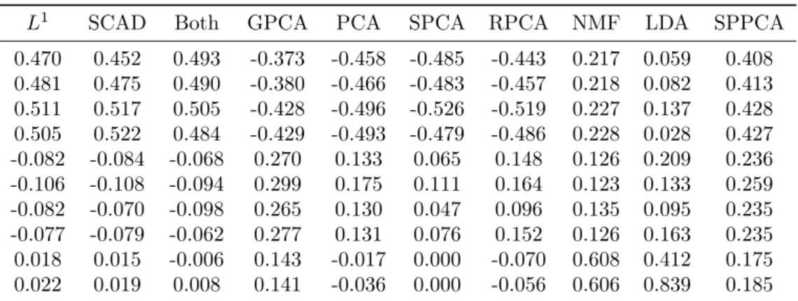
0.470 0.452 0.493 -0.373 -0.458 -0.485 -0.443 0.217 0.059 0.408 0.481 0.475 0.490 -0.380 -0.466 -0.483 -0.457 0.218 0.082 0.413 0.511 0.517 0.505 -0.428 -0.496 -0.526 -0.519 0.227 0.137 0.428 0.505 0.522 0.484 -0.429 -0.493 -0.479 -0.486 0.228 0.028 0.427 -0.082 -0.084 -0.068 0.270 0.133 0.065 0.148 0.126 0.209 0.236 -0.106 -0.108 -0.094 0.299 0.175 0.111 0.164 0.123 0.133 0.259 -0.082 -0.070 -0.098 0.265 0.130 0.047 0.096 0.135 0.095 0.235 -0.077 -0.079 -0.062 0.277 0.131 0.076 0.152 0.126 0.163 0.235 0.018 0.015 -0.006 0.143 -0.017 0.000 -0.070 0.608 0.412 0.175 0.022 0.019 0.008 0.141 -0.036 0.000 -0.056 0.606 0.839 0.185
Table 5.2: Second loading/direction for synthetic data, usingL1 penalised SGPCA, SCAD penalised
SGPCA, the combined penalty SGPCA (both), GPCA, PCA, SPCA, RPCA, NMF, LDA and SPPCA
Analysis of Table 5.1 shows that for each of the three SGPCA variants, the first loading picks a direction corresponding primarily with the second hidden factor, and sec-ondarily with the third hidden factor. Picking out both of these hidden factors together is to be expected, as these two factors are very highly correlated. On the other hand, GPCA’s first loading does not strongly identify a direction associated with any hidden factor. PCA, SPCA and RPCA and SPPCA all have quite similar performance, all find-ing a direction most associated with the third hidden factor, with some contribution from the second. NMF finds a direction primarily associated with the third hidden factor, with a smaller contribution from the second hidden factor. LDA primarily identifies the third hidden factor with a smaller contribution from the first and second; it is worth noting
that the contributions across the same hidden factor appear to vary more than they do in most of the other methods.
Looking at the second loadings/directions in Table 5.2, we see that all three SGPCA variants strongly identify the first hidden factor. GPCA returns a similar loading, but with smaller coefficients for the components of the first hidden factor, and fairly large coefficients (of opposite sign) for the second. It also includes contributions from the third hidden factor. PCA returns fairly similar loadings to GPCA, with slightly larger contributions from the first hidden factor and slightly smaller from the second and third. SPCA and RPCA perform very simiarly to PCA. NMF, on the other hand, produces a loading similar in characteristics to its first loading, strongly identifying the third hidden factor with some contributions from the first and second. LDA also does not identify anything more than its first direction, finding primarily the third hidden factor. SPPCA finds a direction primarily associated with the first component, then with the second, and with a contribution from the third as well.
Of all the algorithms considered, the performance of SGPCA is the closest to the authors’ idealised loadings where we might consider the hidden factors to be related to topics or classifications. Its first loading identifies the second hidden factor and the strongly correlated third hidden factor, and the second identifies the first hidden factor. The second hidden factor, having higher variance than the first, is a sensible choice for the first loading. Given that the third hidden factor has the highest variance we might expect it to dominate the first loading, but we believe that it receives lower coefficients due to its correlation with both of the other hidden factors. Although GPCA, PCA, SPCA and RPCA provide similar identification in the second loading, they all include larger contributions from the second hidden factor, which somewhat reduces interpretability.
5.2. Synthetic Classes
Although SGPCA is an unsupervised dimension reduction method, we believe that its construction should be sufficient to find features sufficient to differentiate between observations drawn from different classes. To investigate this, we performed a similar exercise to that in Section 5.1, but drawing from two different distributions. The first has hidden factors
V1∼Po (25), V2∼Po (25), V3=V1+ 3V2
and the second
V1∼Po (25), V2∼Po (35), V3= 2V1+V2
As in Section 5.1, the first four entries of each vector observation areV1with error, the
second four V2 with error and the last two are V3 with error. We construct all of the
observations by the same method as before. We then perform the same algorithms as before, with the addition this time of MNIR, using as a response the class identifier 0
for the first100 observations and 1 for the second 100. The loadings/directions for all algorithms are given in Table 5.3.
The primary differentiating factors between the two classes of data are the second and third hidden factors. As such, the strong identification of the third hidden factor by all three SGPCA variants is excellent. The first GPCA loading assigns roughly similar
L1 SCAD Both GPCA PCA SPCA RPCA NMF LDA MNIR SPPCA -0.227 -0.196 -0.184 -0.193 -0.123 -0.116 -0.126 0.162 0.198 0.000 0.240 0.042 0.023 0.023 -0.225 -0.110 -0.109 -0.113 0.165 0.263 0.000 0.233 -0.119 -0.101 -0.089 -0.226 -0.127 -0.125 -0.131 0.164 0.098 0.000 0.243 -0.025 -0.030 -0.025 -0.239 -0.120 -0.119 -0.129 0.163 0.183 0.000 0.237 -0.078 -0.069 -0.062 -0.431 -0.130 -0.128 -0.134 0.196 0.245 0.447 0.243 -0.036 -0.058 -0.068 -0.437 -0.130 -0.131 -0.125 0.197 0.208 0.469 0.243 -0.066 -0.042 -0.027 -0.441 -0.129 -0.129 -0.127 0.197 0.174 0.448 0.243 -0.062 -0.053 -0.045 -0.428 -0.126 -0.123 -0.127 0.197 0.097 0.446 0.240 -0.674 -0.682 -0.684 -0.156 -0.656 -0.657 -0.650 0.605 0.307 -0.301 0.515 -0.679 -0.687 -0.691 -0.159 -0.668 -0.670 -0.670 0.610 0.782 -0.300 0.524
Table 5.3: Loadings/directions for classed synthetic data, usingL1 penalised SGPCA, SCAD penalised
SGPCA, the combined penalty SGPCA (both), GPCA, PCA, SPCA, RPCA, NMF, LDA, MNIR and SPPCA.
coefficients to the first and third hidden factors, and slightly higher coefficients to the second. Once again, PCA, SPCA and RPCA give similar loadings, concentrating mostly on the third hidden factor with a smaller contribution for the first and second. NMF also gives highest weighting to the third hidden factor, with smaller contributions from the first and second. SPPCA performs similarly again, though assigns slightly less weighting to the third hidden factor and slightly more to the first two. LDA assigns its highest coefficient to one of the components corresponding to the third hidden factor, but its other coefficients are far more sporadic and inconsistent across the same hidden factor. MNIR’s loading finds a (weighted) difference between the second and third hidden factors.
5.3. Robustness Against Noise
In order to investigate how robust the loadings given by SGPCA are to noise, we will perform a similar synthetic data analysis to that in Section 5.1, but varying the parameter of noise. That is,
V1∼Po (25), V2∼Po (30), V3=V1+ 3V2
We then construct each observation in the usual way, except that the i.i.d. noise for each observation component is instead drawn from a Poisson distribution with meanη and multiplied by1 or−1with equal probability. This is the same setup as previously, except that we can control the variance of the noise. We then find SGPCA loadings for each η ∈ {1,2,3,4}. We again drew 100 observations and performed L1 SGPCA withλL = 107, SCAD SGPCA withλ= 0.1 andλS = 106, and the combined penalty SGPCA with λL = 106, λS = 106 and λ = 0.05. The loadings for the L1 penalised SGPCA are displayed in Table 5.4a, for the SCAD penalised SGPCA in Table 5.4b, and for the combined penalty SGPCA in Table 5.4c.
An examination of Table 5.4a suggests that, for all four magnitudes of noise, the loadings of L1 penalised SGPCA are very similar (up to sign changes), with the first
loading consistently identifying a direction which primarily captures the second and third hidden factors, while the second loading captures the first hidden factor. Table 5.4c
η= 1 η= 2 η= 3 η= 4 η= 1 η= 2 η = 3 η= 4 Loading 1 0.1267 0.0846 0.0355 -0.0182 Loading 2 -0.4553 0.4699 -0.5496 -0.4738 0.1385 0.0941 0.0265 -0.0007 -0.4751 0.4809 -0.4895 -0.5268 0.1303 0.0548 0.0250 0.0473 -0.4807 0.5112 -0.4823 -0.4865 0.1582 0.0454 0.0602 -0.0237 -0.4941 0.5052 -0.4524 -0.4912 0.4128 0.4176 0.4151 -0.4448 0.1482 -0.0824 0.0629 0.0641 0.4150 0.4401 0.4358 -0.3682 0.1402 -0.1060 0.0512 0.0434 0.4012 0.4203 0.5003 -0.4802 0.1534 -0.0816 0.0637 -0.0300 0.4293 0.4452 0.3950 -0.4873 0.1601 -0.0771 0.0684 0.0329 0.3385 0.3417 0.3362 -0.3153 0.0200 0.0181 -0.0454 -0.0777 0.3468 0.3453 0.3352 -0.3098 0.0227 0.0221 -0.0606 -0.0773
(a) Two loadings ofL1penalised SGPCA under varying levels of noise on synthetic data
η= 1 η= 2 η= 3 η= 4 η= 1 η= 2 η = 3 η= 4 Loading 1 0.1266 0.0744 0.0361 -0.0347 Loading 2 -0.4556 0.4524 -0.5505 -0.0414 0.1388 0.0953 0.0262 -0.0237 -0.4753 0.4750 -0.4890 -0.0324 0.1304 0.0580 0.0249 0.0019 -0.4806 0.5168 -0.4826 0.0375 0.1579 0.0517 0.0599 -0.0195 -0.4939 0.5216 -0.4516 -0.0254 0.4126 0.4255 0.4152 -0.0392 0.1481 -0.0843 0.0627 -0.1338 0.4154 0.4339 0.4355 -0.0510 0.1400 -0.1084 0.0514 -0.1471 0.4015 0.4177 0.5005 -0.0430 0.1534 -0.0700 0.0637 -0.1214 0.4287 0.4470 0.3949 -0.0336 0.1601 -0.0792 0.0684 -0.1211 0.3386 0.3414 0.3362 0.8715 0.0202 0.0146 -0.0454 -0.4866 0.3468 0.3452 0.3352 -0.4808 0.0229 0.0195 -0.0606 -0.8303
(b) Two loadings of SCAD penalised SGPCA under varying levels of noise on synthetic data
η= 1 η= 2 η= 3 η= 4 η= 1 η= 2 η = 3 η= 4 Loading 1 0.1267 0.1074 0.0358 -0.0177 Loading 2 -0.4552 0.4933 -0.5501 -0.4747 0.1384 0.0944 0.0263 0.0004 -0.4750 0.4901 -0.4892 -0.5259 0.1303 0.0492 0.0249 0.0469 -0.4807 0.5051 -0.4824 -0.4864 0.1584 0.0318 0.0600 -0.0242 -0.4942 0.4841 -0.4520 -0.4913 0.4129 0.3959 0.4151 -0.4435 0.1483 -0.0684 0.0628 0.0643 0.4149 0.4607 0.4356 -0.3677 0.1403 -0.0936 0.0513 0.0430 0.4011 0.4333 0.5004 -0.4783 0.1533 -0.0980 0.0637 -0.0291 0.4296 0.4412 0.3949 -0.4875 0.1601 -0.0625 0.0684 0.0330 0.3384 0.3304 0.3362 -0.3177 0.0200 -0.0061 -0.0454 -0.0785 0.3467 0.3398 0.3352 -0.3124 0.0226 0.0082 -0.0606 -0.0777
(c) Two loadings of the combined penalty SGPCA under varying levels of noise on synthetic data
Table 5.4: Investigations of the performance of all three SGPCA variants across varying levels of noise.
suggests that the combined penalty SGPCA has the same characteristics. However, Table 5.4b suggests that the SCAD penalised SGPCA is not quite so robust; both loadings seem to vary more asη increases, with the loadings for η= 4being very different from those forη= 1, no longer giving near-equal weights amongst components corresponding to the same hidden factors. This is, perhaps, not surprising, given the use of theL1 penalty in RPCA and JSPCA for its robustness to outliers (which become more probable with increasing magnitude of noise).
5.4. Dependence on Tolerance
In our anecdotal experience of estimating the SGPCA approximation across a variety of datasets, we found that decreasing the numerical tolerance increased the time taken to complete the algorithm approximately exponentially. As this could quickly become untenable, we performed a further simulation study to examine the effects of the tolerance on the accuracy of the solution. The data was generated in precisely the same way as in Section 5.1 and the same three SGPCA variants were fitted with the same parameters, varying only the tolerance. We chose a range of values between10−4 and 10−9, taking the results of the latter as the “gold standard” by which we judged the accuracy.
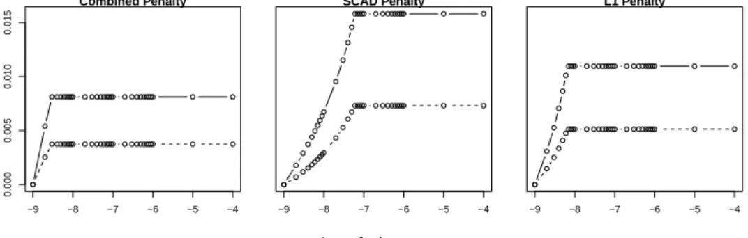
In Figure 5.1a we graph the Euclidean distances of each of the two loadings from each run of the algorithm against the logarithm of the chosen tolerances. As an alternative measure, in Figure 5.1b we show the deviances from each fit, “normalised” by division by the deviance of our gold standard fit. Both figures show that tolerances too large provide fits which are nearly identical, having had only a few iterations. Beyond a critical tolerance, the fits quickly converge to the gold standard fit. However, we wish to draw attention to the axes of both plots – the largest deviance amongst all fits is less than one half of one percent larger than the gold standard, and the Euclidean distance between the gold standard and the fit further from it is of order 10−2. We suggest, therefore, that a practical strategy for choosing a tolerance value would be to choose the smallest value that allows feasible optimisation times, preferably (if this study is representative) smaller than10−7.
6. Healthcare Data
The dataset we analysed is a by-product of a lexicon-based classifier which the health board developed in response to a need to systematically classify letters sent by consul-tants to GPs and patients. It consists of just over 40,000 exemplar sentences generated procedurally from a set of seeds. All observations are labelled either discharge or follow-up with a heavy imbalance in favour of follow-follow-up; this imbalance is due to the nature of the problem being addressed, and approximates the expected imbalance in the col-lection of letters. For the analysis we drew a stratified sample of 200 observations from the dataset to calculate the projection matrices for each method. The dimension of the chosen data was 55 in this case. We then drew 50 observations from each of the two classes to use as a testing dataset, and show the results of applying the projections to this test set in Figure 6.1. For each algorithm, we plot each pair of the first three prin-cipal components. Each plot shows the 100 selected points coloured (and with different point characters) according to the class. Due to the similar performance of the three types of SGPCA, we performed only theL1penalised version. We also show GPCA and
(a) Euclidean distances between loadings from fits with different tolerance values for each of the SGPCA variants. The first loading is shown dashed, and the second is shown solid.
−9 −8 −7 −6 −5 −4 0.000 0.005 0.010 0.015 Combined Penalty −9 −8 −7 −6 −5 −4 SCAD Penalty −9 −8 −7 −6 −5 −4 L1 Penalty Log of tolerances Distance
(b) Deviances from each fit across a range of tolerance values, divided by the deviance from the fit with the smallest tolerance. All three SGPCA variants are shown.
−9 −8 −7 −6 −5 −4 1.0000 1.0005 1.0010 1.0015 Combined Penalty −9 −8 −7 −6 −5 −4 SCAD Penalty −9 −8 −7 −6 −5 −4 L1 Penalty Log of tolerances De viance
Figure 5.1: Behaviour of all SGPCA variants as tolerance is varied.
−4 −2 0 2 4 6 −4 −2 0 2 Component 1 Component 2 −4 −2 0 2 4 6 −4 −2 0 2 4 Component 1 Component 3 −4 −2 0 2 −4 −2 0 2 4 Component 2 Component 3
(a)L1 penalty SGPCA
−12 −10 −8 −6 −4 −2 0 −4 −2 0 2 4 6 Component 1 Component 2 −12 −10 −8 −6 −4 −2 0 −6 −4 −2 0 2 4 Component 1 Component 3 −4 −2 0 2 4 6 −6 −4 −2 0 2 4 Component 2 Component 3 (b) GPCA 0.0 0.5 1.0 1.5 2.0 −0.5 0.0 0.5 1.0 1.5 Component 1 Component 2 0.0 0.5 1.0 1.5 2.0 −1.0 −0.5 0.0 0.5 1.0 Component 1 Component 3 −0.5 0.0 0.5 1.0 1.5 −1.0 −0.5 0.0 0.5 1.0 Component 2 Component 3 (c) PCA
Figure 6.1: Plots of pairs of the first three principal components for the healthcare dataset obtained from SGPCA, GPCA and PCA.
PCA as the most comparable and most widely used algorithms respectively; the other algorithms are omitted due to a combination of lack of space and poor performance. Qualitatively, all three algorithms have reasonably similar performance, allowing decent linear separation of the data. This suggests that our algorithm seems to inherit PCA’s reputation for frequently providing useful loadings for analysing with respect to some response variable, despite not using such information itself.
7. Discussion
In this paper we have introduced a sparsifying penalty to the generalised principal components of Landgraf and Lee (2015), along with an efficient routine by which to calculate the loadings. By means of simulation and case study we have shown excellent performance in estimating appropriate (and useful) principal component loadings, giving arguably the best loadings in the synthetic cases and projections on par with the current state of the art for text in the healthcare study.
Comparison of the efficacy of the three penalties we used (L1, SCAD andL1+ SCAD) suggest little difference between them. As such, our preference is for theL1 penalty due
both to its simplicity and its reliance on only one tuning parameter, unlike the SCAD penalty which has two and the combination of both which has three.
It is worth noting that, as with all non-convex problems, our method will likely have multiple minima. One way this could be mitigated, should it prove problematic, is to repeatedly run the optimisation procedure from a variety of initial values and choose between the found optima by means of the deviance. However, the authors’ experience is that using Gaussian PCA as the starting point is both convenient (as it provides a left semi-orthogonal matrix) and effective; the optima the optimisation procedure finds from this starting point have consistently exhibited the properties we desire.
There is significant scope for extension of this work. Firstly, one can look into a data-driven method for choosing the optimum values ofλL, λandλS. Secondly, there is scope for investigating other penalty functions, such as theL0 penalty, to better under-stand how penalising the coefficients drives sparsity. Another possible extension is the development of methods for supervised dimension reduction, extending existing methods such as partial least squares. Finally, a more challenging problem is the development of kernel-based GPCA and SGPCA for non-linear feature extraction.
Acknowledgements
The authors would like to thank Cardiff and Vale University Health Board for sup-porting the project and allowing access to the healthcare dataset. We are also deeply grateful for the insightful comments provided by the reviewers and editor, this article is much improved for their efforts.
A1. Derivation of deviance
The deviance of our model from the saturated model is properly D(X|Θ) =−2logP(X|Θ)−logPX|Θ˜
where Θ˜ is the matrix of saturated parameters for each observation. However, as we seek only value ofΘwhich minimises the deviance, we can disregard the contribution of the log probability from the saturated model, as well as the factor of2. This leaves the expression for the pseudo-deviance as
D(X|Θ) =−logP(X|Θ) =−log n Y i=1 h(xi) exp xTiθi−b(θi) =− n X i=1 logh(xi) +xiTθi−b(θi) = n X i=1
b(θi)−xTi θi (with an additive constant)
= n X i=1 p X j=1
{bj(θij)−xijθij} (using the independence of each component)
This can then be recognised as the expression in (1) by substituting in the appropriate form forθij.
A2. Derivation of optimality conditions
In order to derive optimality conditions, we need first to construct the Lagrangian of the problem.
L(U,µ)..=S(U,µ) + Tr Λ UTU−I
whereΛis an l×l symmetric matrix of Lagrange multipliers which we use in order to capture the semi-orthogonality ofU, andS(U,µ)is given in (5). Calculating the partial derivatives with respect toU,µand Λwe arrive at the following first-order optimality conditions, the derivations of which can be found below.
n X i=1 p X j=1 b0j µj+ h UUTθ˜i−µ i j −xij δrjUT[l] ˜ θi−µ +Ujs ˜ θir−µr +λLsgn (Urs) +λSPS0 (|Urs|) sgn (Urs) + 2ΛTl Ur= 0 r= 1, . . . , n, s= 1, . . . , p (B.1) n X i=1 p X j=1 b0j µj+ h UUTθi˜ −µi j −xij δjr− UUTjr= 0 r= 1, . . . , n (B.2) UTU = I (B.3)
whereAiindicates theith row andA[i] theith column of the matrixA(where both are
that, due to the non-differentiability of the absolute value function at0, (B.1) only holds forUrs6= 0. We begin by deriving (B.1). ∂ ∂Urs ( n X i=1 p X j=1 ( bj µj+ h UUTnθ˜i−µ oi j −xij µj+ h UUTnθ˜i−µ oi j +λSPS(|Uij|) ) +λL|U|+ Tr Λ UTU−I ) = n X i=1 p X j=1 b0j µj+ h UUTnθ˜i−µ oi j −xij ∂ ∂Urs µj+ h UUTnθ˜i−µ oi j +λSPS0 (|Urs|) sgn (Urs) +λLsgn (Urs) + ∂ ∂Urs Tr Λ UTU−I = n X i=1 p X j=1 b0j µj+ h UUTnθi˜ −µoi j −xij δrjUT[s] h ˜ θi−µi | {z } (∗) + Ujs h ˜ θir−µr i | {z } (†) +λSPS0 (|Urs|) sgn (Urs) +λLsgn (Urs) + 2ΛTlUr | {z } (‡)
Where(∗)comes from the terms quadratic inUrs,(†)is from the terms linear inUrs, and
(‡)is from the summation definition of the trace. Setting the above equation equal to0
for each value ofr∈1, . . . , nands∈1, . . . , pyields the first set of first order optimality conditions. Similarly, we derive the next set by differentiating with respect to therth
element ofµ. ∂ ∂µr ( n X i=1 p X j=1 ( bj µj+ h UUTnθ˜i−µ oi j −xij µj+ h UUTnθ˜i−µ oi j +λSPS(|Uij|) ) +λL|U|+ Tr Λ UTU−I ) = n X i=1 p X j=1 b0j µj+ h UUTnθi˜ −µoi j −xij ∂ ∂µr µj+ h UUTnθi˜ −µoi j = n X i=1 p X j=1 b0j µj+ h UUTnθ˜i−µ oi j −xij δjr− ∂ ∂µr UUTµ j = n X i=1 p X j=1 b0j µj+ h UUTnθi˜ −µoi j −xij n δjr− UUTjro
Once again, setting the final expression equal to0for each value ofrgives theµoptimality conditions. Finally, theΛoptimality condition is easily derived, this time using matrix
differential calculus for convenience. ∂ ∂Λ ( n X i=1 p X j=1 ( bj µj+ h UUTnθi˜ −µoi j −xij µj+ h UUTnθi˜ −µoi j +λSPS(|Uij|) ) +λL|U|+ Tr ΛUTU−I ) = ∂ ∂ΛTr Λ UTU−I = vec UTU−I
Setting this equal to0reduces toUTU = I, the semi-orthogonality condition.
A3. Derivation of gradients
Calculating the gradients of the majorised objective function is very similar to calcu-lating the first order optimality conditions in Appendix A2, as the terms fromD(X,U,µ)
will be the same. Further, the perturbed penalty has no terms inµ, so theµ-gradient is precisely ∂∂µD(X,U,µ), so this gradient will not be recalculated. This simply leaves calculating ∂U∂ rsM ε P U|U(t−1) ∂Mε P ∂Urs = ∂ ∂Urs n X i=1 p X j=1 ( λL U (t−1) ij +λSPS U (t−1) ij + U2 ij− U(ijt−1) 2h λL+λSPS0 U (t−1) ij i 2hε+ U (t−1) ij i ) = n X i=1 p X j=1 ∂ ∂Urs U2ij−U(ijt−1) 2λL+λSPS0 U (t−1) ij 2hε+ U (t−1) ij i = 2Urs λL+λSPS0 U (t−1) rs 2hε+ U (t−1) rs i
We omit the arguments ofλ, atoPS for notational convenience.
A4. Derivation of SCAD penalty from derivative The SCAD penalty derivative (2) is equivalently given as
p0(θ) = λ 0< θ≤λ aλ−θ a−1 λ < θ < aλ 0 aλ < θ
Computingp(θ)is then a matter of integrating carefully. For0< θ≤λ,p(θ) =R0θλdt= λθ. Forλ < θ≤aλ, p(θ) =p(λ) + Z θ λ aλ−t a−1 dt=λ 2+ aλt−1 2t 2 a−1 t=θ t=λ =−θ 2−2aλθ+λ2 2(a−1)
Finally, foraλ < θ,p(θ) =p(aλ) +Raλθ 0dt=p(aλ) = (a+1)2 λ2. Together, this gives (3).
References
Blei, D. M., Ng, A. Y., Jordan, M. I., 2003. Latent dirichlet allocation. Journal of machine Learning research 3, 993–1022.
Collins, M., Dasgupta, S., Schapire, R. E., 2002. A Generalization of Principal Components Analysis to the Exponential Family. Advances in Neural Information Processing Systems 14, 617–624.
de Leeuw, J., 2006. Principal component analysis of binary data by iterated singular value decomposition. Computational Statistics & Data Analysis 50 (1), 21–39.
Diederichs, E., Juditsky, A., Nemirovski, A., Spokoiny, V., 2013. Sparse non Gaussian component analysis by semidefinite programming. Machine Learning 91, 211–238.
Ding, C., He, X., 2004. K-means clustering via principal component analysis. In: Proceedings of the twenty-first international conference on Machine learning. ACM, p. 29.
Fan, J., Li, R., 2001. Variable Selection via Nonconcave Penalized Likelihood and its Oracle Properties. Journal of the American Statistical Association 96 (456), 1348–1360.
Gillis, N., 2014. The Why and How of Nonnegative Matrix Factorization. ArXiv e-prints.
Guan, Y., Dy, J., 2009. Sparse probabilistic principal component analysis. In: Artificial Intelligence and Statistics. pp. 185–192.
Hoerl, A. E., Kennard, R. W., 1970. Ridge Regression: Biased Estimation for Nonorthogonal Problems. Technometrics 12 (1), 55–67.
Hotelling, H., 1933. Analysis of a complex of statistical variables into principal components. Journal of Educational Psychology 24 (6), 417–441.
Hu, Z., Pan, G., Wang, Y., Wu, Z., 2016. Sparse principal component analysis via rotation and trunca-tion. IEEE transactions on neural networks and learning systems 27 (4), 875–890.
Hunter, D. R., Li, R., 2005. Variable selection using MM algorithms. Annals of Statistics 33 (4), 1617– 1642.
Kwak, N., 2008. Principal component analysis based on l1-norm maximization. IEEE transactions on pattern analysis and machine intelligence 30 (9), 1672–1680.
Landgraf, A. J., Lee, Y., 2015. Generalized Principal Component Analysis : Projection of Saturated Model Parameters. Ohio State University Statistics Department Technical Report 892 (892). Lu, M., Huang, J. Z., Qian, X., 2016. Sparse exponential family Principal Component Analysis. Pattern
Recognition 60, 681–691.
Nocedal, J., Wright, S., 2006. Numerical optimization. Springer Science & Business Media.
Pearson, K., 1901. On lines and planes of closest fit to systems of points in space. The London, Edinburgh, and Dublin Philosophical Magazine and Journal of Science 2 (1), 559–572.
R Foundation for Statistical Computing, Vienna, 2011. R Development Core Team. R: A Language and Environment for Statistical Computing 55, 275–286.
Schönemann, P. H., 1966. A generalized solution of the orthogonal procrustes problem. Psychometrika 31 (1), 1–10.
Taddy, M., 2013. Multinomial Inverse Regression for Text Analysis. Journal of the American Statistical Association 108 (503), 755–770.
Taddy, M., 2015. Distributed multinomial regression. The Annals of Applied Statistics 9 (3), 1394–1414. Tibshirani, R., 1996. Regression Shrinkage and Selection via the Lasso. Journal of the Royal Statistical
Society. Series B (Methodological) 58 (1), 267–288.
Tipping, M. E., Bishop, C. M., 1999. Probabilistic Principal Component Analysis. Journal of the Royal Statistical Society. Series B (Statistical Methodology) 61 (3), 611–622.
Wen, Z., Yin, W., 2013. A feasible method for optimization with orthogonality constraints. Mathematical Programming 142 (1-2), 397–434.
Zou, H., Hastie, T., 2005. Regularization and Variable Selection via the Elastic Net. Journal of the Royal Statistical Society. Series B (Methodological) 67 (2), 301–320.
Zou, H., Hastie, T., Tibshirani, R., 2006. Sparse Principal Component Analysis. Journal of Computa-tional and Graphical Statistics 15 (2), 265–286.