Image Labeling and Classification by Semantic Tag Analysis

(1)

Ugur Kirbac

Image Labeling and Classification by Semantic Tag

Analy-sis

Master of Science Thesis

Supervisors: Esin Guldogan and Moncef Gabbouj

Supervisors and topic were ap-proved by Faculty of Computing and Electrical Engineering Coun-cil on Aug 15, 2012.

(2)

ABSTRACT

TAMPERE UNIVERSITY OF TECHNOLOGY Master’s Degree Program in Information Technology

KIRBAC, Ugur: Image Labeling and Classification by Semantic Tag Analysis Master of Science Thesis, 52 pages

May 2013

Major Subject: Signal Processing

Supervisors: Prof. Moncef Gabbouj and Dr. Esin Guldogan

Keywords: Image labeling, classification, semantic text analysis, WordNet

Image classification and retrieval plays a significant role in dealing with large mul-timedia data on the Internet. Social networks, image sharing websites and mobile appli-cation require categorizing multimedia items for more efficient search and storage. Therefore, image classification and retrieval methods gained a great importance for re-searchers and companies.

Image classification can be performed in a supervised and semi-supervised manner and in order to categorize an unknown image, a statistical model created using pre-labeled samples is fed with the numerical representation of the visual features of imag-es.

A supervised approach requires a set of labeled data to create a statistical model, and subsequently classify an unlabeled test set. However, labeling images manually requires a great deal of time and effort. Therefore, a major research activity has gravitated to-wards finding efficient methods to reduce the time and effort for image labeling. Most images on social websites have associated tags that somewhat describe their content. These tags may provide significant content descriptors if a semantic bridge can be es-tablished between image content and tags. In this thesis, we focus on cases where accu-rate class labels are scarce or even absent while some associated tags are only present. The goal is to analyze and utilize available tags to categorize database images to form a training dataset over which a dedicated classifier is trained and then used for image classification. Our framework contains a semantic text analysis tool based on WordNet to measure the semantic relatedness between the associated image tags and predefined class labels, and a novel method for labeling the corresponding images. The classiﬁer is trained using only low-level visual image features. The experimental results using 7 classes from MirFlickr dataset demonstrate that semantically analyzing tags attached to images significantly improves the image classification accuracy by providing additional training data.

(3)

PREFACE

I have no special talent. I am only passionately curious. Albert Einstein This thesis concludes my Master of Science in Information Technology in the de-partment of Signal Processing, Tampere University of Technology, Finland.

I would like to convey my sincere gratitude to my supervisor Dr. Esin Guldogan and examiner Professor Moncef Gabbouj and for giving me the opportunity for this work and their guidance, motivation and support. In addition, I would also like to thank Pro-fessor Serkan Kiranyaz for his time spent on technical discussions and teachings. Dur-ing the process of experiments and writDur-ing of the thesis, Stefan Uhlmann was a very good friend who gave his professional comments as well as motivational advice on my work.

Finally, my family that supported me from the beginning to the end of my education in Finland, I would like to thank my family for their concerns, especially my mother for about my health, my father about my expenses and my brother about my social life.

Tampere, FINLAND, May 2013. Ugur KIRBAC

(4)

Table of Tables

Table 2-1 MUVIS multimedia family ... 16

Table 2-2 MUVIS image types ... 16

Table 3-1 Pseudo code for scoring algorithm ... 33

Table 4-1 Pseudo code of the automatic labeling framework. ... 38

Table 5-1 The features and parameters used for image classification ... 40

Table 5-2 Predefined class sentences ... 41

Table 5-3 Precision of images labeled per class. ... 42

Table 5-4 Classification performances over the test set using ground truth training datasets with different sizes ... 43

Table 5-5 Classification performances over the test set using the training datasets automatically created using the proposed framework ... 44

Table 5-6 Retrieval results for ground truth ... 45

(6)

Table of Figures

Figure 1-1 The overview of the main framework ... 2

Figure 2-1 The flowchart of a supervised machine learning application ... 7

Figure 2-2 Left: Binary classification Right: 3-class classification ... 8

Figure 2-3 A simple coincidence matrix ... 8

Figure 2-4 Topology of CNBC framework ... 10

Figure 2-5 The original image... 12

Figure 2-6 3 to 8 Dominant color image ... 12

Figure 2-7 Sample textures ... 13

Figure 2-8 The main view with all the functionalities of DBS Editor ... 17

Figure 2-9 Parameter selection for feature extraction ... 18

Figure 2-10 A snapshot of retrieval window of Mbrowser ... 19

Figure 2-11 Interaction of Fex Module with MUVIS Applications ... 22

Figure 2-12 Demonstration of M-MUVIS system architecture ... 23

Figure 2-13 Query process in M-MUVIS ... 24

Figure 3-1 An Example of the syponym saxonomy in WordNet ... 29

Figure 3-2 The Flowchart of semantic similarity between swo sentences... 32

Figure 4-1 Tags: ford, 1965, mustang, car ... 34

Figure 4-2 Traditional way of labeling by an expert. ... 35

Figure 4-3 Proposed labeling by automatic labeling framework. ... 35

Figure 4-4 A sample database of six images with associated tags ... 36

Figure 4-5 The illustration of the image labeling mechanism ... 37

Figure 4-6 The classification scheme with the Random Forest. ... 39

Figure 5-1 A visual representation of a class vector, as the red tone gets lighter the confidence of labeling decreases. This heterogenic representation facilitates the training set creation. ... 42

(7)

Abbreviations and Acronyms

AFeX Audio Feature Extraction

ANMRR Average Normalised Modified Retrieval Rank

API Application Programming Interface

AVR Average Rank

CBIR Content Based Image Retrieval

CEO Chief Executive Officer

CPU Central Processing Unit

DC Dominant color

DCD Dominant Color Descriptor

DLL Dynamic Linked Library

FeX Feature Extraction

FV Feature Vector

GPS Global Positioning System

GUI Graphical User Interface

GTD Ground Truth Data

HCT Hierarchical Cellular Tree

HSV Hue Saturation Value

HTTP Hypertext Transfer Protocol

MAM Metric Access Method

ML Machine Learning

MPEG Moving Picture Experts Group

NMRR Normalised Modified Retrieval Rank

NQ Normal Query

PAM Point Access Method

PQ Progressive Query

QbE Query by Example

QbR Query by Region

QbS Query by Subject

RAM Random-access Memory

SAM Spatial Access Method

SEG Segmentation

SSL Semi-supervised learning

YUV Luminance-Bandwidth-Chrominance

(8)

1. INTRODUCTION

Pattern recognition is a collection of tools, algorithms and methods used for predict-ing the actual identity of a given unknown input such as image, video or text. Classifica-tion is an instance of pattern recogniClassifica-tion that determines to which predefined class a given unknown input belong. For example, it can answer whether a given fruit is apple or banana using the statistical data of fruits.

Classification narrows down towards image classification that deals with only imag-es whose content is predicted using a statistical model formed with the numerical repre-sentation of the visual features of images. This kind of approach is known as supervised approach that requires a certain set of labeled samples. In supervised learning, a classi-fier is trained with the manually labeled (training) dataset and the aim is then to classify the unlabeled examples in the test set. One can expect a higher classification perfor-mance as the size of the training dataset increases. In real cases, obtaining a certain set of training data is cumbersome process and takes much time of experts. Our motivation is to reduce the cost of the image labeling process for content-based image classification and retrieval.

Nowadays, user-created tags are available on social media websites such as Flickr. These tags are a useful data source without any expense for researchers. The research conducted on the use of Flickr show that users are eager to provide this semantic con-text through manual annotations [1]. In addition to describing the content of an image, tags might contain irrelevant words. Moreover, associated metadata attached to the im-age can also be used as the assistive textual information.

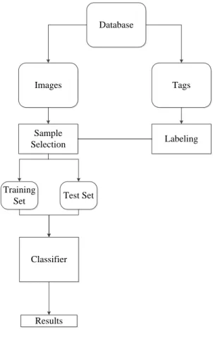
In this thesis, we have presented an approach to utilize tags associated with images for content-based image classification. Fundamentally, visual features and tags are two different but tightly related image descriptors, and in order to utilize both the visual in-formation and user-created tags for image classification, we need to deal with two main challenges. The first challenge is to analyze tags semantically with an efficient and ac-curate text analysis algorithm to extract the acac-curate content labels and the second chal-lenge is to establish a robust and effective bridge to use the semantic relationship for image classification. Figure 1-1 shows the general overview of the proposed framework. The mechanism starts with splitting the tag sets from the images in the database. The tags are analyzed and labeled with the categories in a predefined vocabulary. As a re-sult, a training set is created for learning the image classifier. This training set is formed with no expense, in other words, no manual work has been used to label the images.

(9)

Tags Images Database Labeling Sample Selection Classifier Results Training

Set Test Set

Figure 1-1 The overview of the main framework

Various approaches based on textual information have been proposed for visual classification tasks. For example, Jin et al [2] employed WordNet [3] ontology for re-moving irrelevant keywords produced during the process of image annotation. They investigate various semantic similarity measures between keywords and determine the correlation between associated keywords (tags) and the visual segments in images. Srikanth et al. [4] performed automatic image annotation by generating a visual vocabu-lary using WordNet ontology. Cho et al. [5] examined the conceptual relationship be-tween keywords associated with images. They utilize WordNet hierarchy to find the semantic relationship between keywords in annotated images. After measuring the rela-tionship, they removed irrelevant keywords from the whole keyword set and bridged the semantic gap between image content and the tags. The most related prior works are the two recent papers, [6] [7] both of which use the tags as the assistive information to im-prove the performance of the content-based image classification.

Wang et al. [7] formed a textual representation of the untagged images in a dataset that contains around one million tagged and untagged images. Their approach is using the visual features to obtain the textual data and they perform object-based image classi-fication. Our approach differs in that we do not construct a new textual image represen-tation. However, we both expect that textual features to capture the semantics of images and help to the image content analysis. In addition, we use only associated tags to obtain examples to train a classifier that uses only low-level visual features.

(10)

The work in [6] used a semi-supervised technique, which exploits the textual infor-mation by fusing with visual features to train a classifier. Their system contains two different classifiers. The first one was trained with both visual content and tags of the images and is used to label the unlabeled training set. Then the output of the first classi-fier was added to the existing training set for learning the second classiclassi-fier.

The rest of the thesis is organized as follows. Section 2 describes content-based im-age classification and retrieval. Semantic analysis of sentences is explained in Section 3. The proposed framework is described in Section 4; we explain how image labeling is performed by semantic analysis of tags attached to images and the use of the labeled images for image classification. In Section 5, we demonstrate the experimental results of the proposed method. Finally, conclusions and future work are given in Section 6.

(11)

2. CONTENT-BASED IMAGE CLASSIFICATION

AND RETRIEVAL

Content-based image classification is a significant step in image indexing and re-trieval area. Content-based image rere-trieval (CBIR) methods were first proposed in the early 1990s [8]and researchers have studied on various methods to improve the accura-cy of both classification and retrieval. These content-based methods have become more popular than text-based image retrieval methods, which are very subjective and noisy because of their use of human-created keywords, and very expensive because of manual processing. The goal of CBIR is to produce the best retrieval results corresponding to human concepts.

2.1. Classification and Learning Types

2.1.1. Overview on Machine Learning

Learning and intelligence are hard to define as they consist of complicated and mul-tiple processes. Merriam-Webster [9] defines “learn” as follows: “To gain knowledge, or understanding of, or skill, by study, instruction or experience / and modification of a behavioral tendency by experience”. Zoologists and psychologists have studied learning in animals and people but here leaning in machines is more important, although there are some similarities between learning in animals and machines. As we know, psy-chologists have made computational models of their theories on animal and human learning and these techniques have then been transferred and used for machine learning. Some of the techniques and concepts researchers are looking at in the area of machine learning could also highlight forms of biological learning [10] .

The process of programming computers to learn is known as Machine Learning [10]. Computers are utilized for a wide set of tasks. For programmers designing and implementing the correct software is not overly challenging, although there are various tasks and these tasks can be organized into four categories.

First, no human experts exist for certain problems such as in modern automated manufacturing facilities where it does no good to study sensor readings in order to pre-dict machine failures before they happen. This is due to the machines being new, so no knowledge can be communicated to a programmer to build a computer system. Whereas a machine learning system could analyze data and problems and learn to predict what causes the problems. In addition, there are problems where human experts exist espe-cially in many areas of perceptual tasks where human experts exist such as speech and

(12)

handwriting recognition as well as natural language comprehension. Almost everyone has expert-level abilities in these areas but cannot explain the route they follow when undertaking the tasks. Luckily, machines can be given examples of the inputs and cor-rect outputs for these tasks, so machine learning algorithms can learn to map the inputs to the outputs.

On the other hand, problems also exist where there is fast changing phenomena. For example, people would like to be able to predict the future behavior of the stock market, consumer purchases, or of exchange rates. These financial fields change so often that despite hopes of constructing a program that is able to predict these changes is almost impossible, as it would also require rewriting. A program that learns can help by contin-ually modifying and tuning rules it has learnt to predict.

Furthermore, certain applications require separate customization for each user. A good example of this is a filter program to distinguish unwanted emails from useful ones. Each user will require their own different filters as it would be ludicrous to ask each user to program their own rules. It would also be impractical to supply each user with a software engineer to continually update the latest rules. A machine learning sys-tem, which would recognize which mails, is rejected and which are stored can decipher the filtering rules.

Research questions in the fields of statistics, data mining, psychology as well as ma-chine learning deals with the same questions albeit with a different emphasis /focal point [11].

Statistics concentrates on understanding the phenomena that have generated the da-ta, often with the goal of testing various hypotheses about the phenomena in question. Data mining seeks to locate comprehensible patterns in the data.

Psychological studies of human learning seek to comprehend the mechanisms that are the basis of the various learning behaviors exhibited by people (concept learning, skill acquisition, strategy change, etc.) [12] .

As we can determine from the discussion on applications, the range of learning problems is extensive. However, researchers have identified multiple templates that can be applied in numerous situations. These templates make deployment of machine learn-ing in practice easy and our discussion will largely focus on a choice set of such prob-lems. We now give a by no means complete list of templates.

Machine Learning (ML) presents a number of applications, most importantly in data mining field. Machine learning can be used where multiple discover the relationship between multiple features [13]. Databases are created with the items that have the same kind of features. Considering pattern recognition systems, two types of learning mecha-nisms are very important: Supervised and Unsupervised Learning (instead of learning, classification can be used interchangeably in pattern recognition field). Unsupervised learning uses unlabeled items in a database whereas supervised learning is carried out if the items are labeled. Unsupervised algorithms result unknown but beneficial classes of instances whereas supervised learning requires predefined classes before classification [14].

(13)

2.1.2. Supervised and Unsupervised Learning and Classification

Unsupervised Learning algorithms do not require any labeled data that, in contrast, is the prerequisite for supervised learning algorithms. It seeks the hidden information of a bunch of unlabeled data. In theory, this type of learning does not have evaluation cri-teria since the input is unknown. One of the most commonly used types of unsupervised algorithms is clustering [14]. Clustering methods simply computes the similarity be-tween instances to collect them into different groups. Various distance metrics exist in the literature and Euclidean is one of the most commonly used metric. Euclidean dis-tance [15] between two n- dimensional feature spaces gives the numerical similarity measure of two patterns [16]. Researchers gravitate towards clustering because of sev-eral reasons:

 The collection and manually categorizing the training data set can be costly and time consuming.

 In some cases for data mining, natural clusters are chosen over manually created ones.

 The properties of feature vectors can vary as the database grows. Especially, in medical image classification area, testing data set might be different from the training data used for the classifier in the beginning.

Theoretically speaking, a set of feature vectors can be defined as

D = (1) Clustering problem is that grouping each feature vector into a cluster with a fixed and predefined size as c.

(2) (3)

For all i ≠ j, we need some further assumptions for the problem to be sensible. (An arbi-trary division of D into different classes is not likely to be useful.) Here, we assume that we can measure the similarity of any two feature vectors somehow. Then, the task is to maximize the similarity of feature vectors within a class. For this, we need to be able to define how similar are the feature vectors belonging to some set Di.

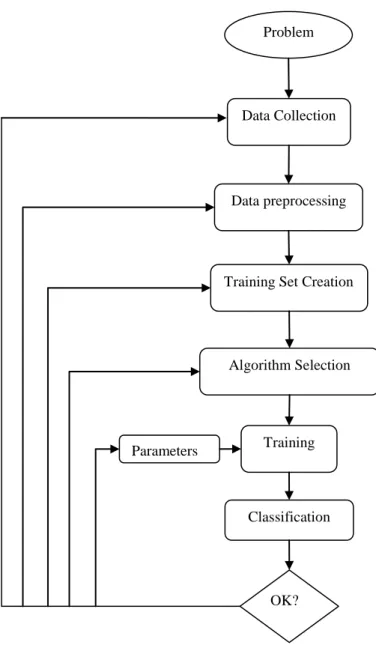
Supervised learning is the process of learning a set of rules from manually labeled data so called training set. The purpose is creating a classifier that uses the small portion of a database as training set and uses the big portion of the database as test set. The flowchart of supervised ML application for a real-world problem is demonstrated in Figure 2-1. The first step is collecting the dataset, which is very expensive in some

(14)

cas-es. Mostly, an expert in the field suggests which fields (attributes, features) are the most informative [13].

Semi-supervised learning (SSL) stands between supervised and unsupervised learning. In addition to unlabeled data, the algorithm is given some supervision infor-mation, mostly for labeled examples. In this case, the dataset X =(xi)∈[n]can be divided into two parts: the points X1:=(x), for which labels Y1:=(y1,...,yn) are provided, and the points Xu:=(x), the labels of which are not known [13]..

One the most commonly studied issue in machine learning field is possibly Bina-ry Classification [17]. It has been used for a great deal of significant developments for a long time. Actually, the basic question is to which random variable ∈ a pattern

Problem

Data Collection

Data preprocessing

Training Set Creation

Algorithm Selection

Training

OK? Classification Parameters

(15)

x in X domain will be assigned. For example, given samples of cards on which are im-ages of cherries and bananas, we want to categorize if the object is cherry or banana. Examples can be derived, however understanding the basic problem will help us to fig-ure out most of the practical issues.

.

Figure 2-2 Left: Binary classification Right: 3-class classification

In the 3-class classification case that is illustrated in Figure 2-2, vagueness is higher. For example, separating the diamonds from triangles is not enough alone to categorize the objects accurately because we also have to separate the diamonds from the stars.

Multiclass classification deals with categorization of more than two classes. The fundamental distinction is that ∈ can assume multiple values. For example, music can be divided into different genres such as art music, traditional music, and pop-ular music based on the composers. The critical level of the error depends on the possi-ble consequences. For example, in medical field, the significance of the accuracy is higher than e-mail spam classification [10].

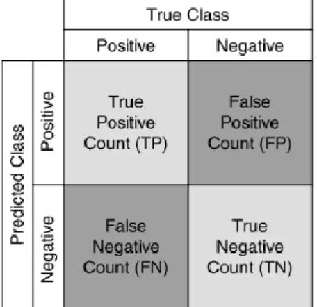
In classification problems, performance measurements are carried out with the aid of coincidence matrix. Figure 2-3 demonstrates a generic coincidence matrix for a binary classification problem [18].

Figure 2-3 A simple coincidence matrix

True outputs are demonstrated by lighter color while false decisions (errors) are dimmed. The true positive rate of a classifier is calculated by dividing the number of accurately categorized positives (the true positive count) by the total number of positives. The false positive rate of the classifier is calculated by dividing

(16)

the inaccurately categorized negatives (the false negative count) by the total number of negatives.

The overall accuracy of a classifier is calculated by dividing the total accurately categorized positives and negatives by the total number of patterns [18]. Below are the performance evaluation formulas.

True Positive Rate (4)

True Negative Rate (5)

Accuracy

(6)

Precision (7)

Recall (8)

 True positive (tp) – a pattern classified as class n that really was.

 True negative (tn) – a pattern classified as not class n, and really was not.

 False negative (fn) – a pattern classified as not class n, though it really was.

 False positive (fp) – a pattern classified as class n, though it was not.

2.1.3. CNBC: Incremental Evolution of Collective Network of Binary Classifier (CNBC)

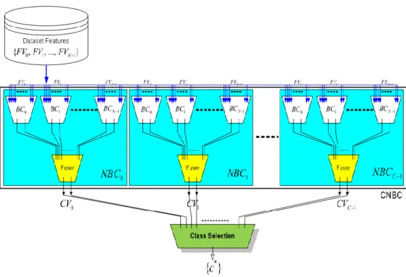
A number of image classifiers have been studied and the collective network of bina-ry classifier developed by Serkan et al. has been used in our experiment [19]. The unique characteristic of this classifier is that it does not need a complete training data in the beginning of the training. It creates a number of networks of binary classifiers (NBCs) to discriminate each category and optimal binary classifier is chosen in each of the NBCs by evolutionary search. Visual and digital performance measurements of the framework proved that this system is accurate and efficient for scalable CBIR and clas-sification. In order to increase classification accuracy that leads to an improvement of the CBIR performance, a global framework that represents a collective network of evo-lutionary classifiers is used. This approach creates an assigned classifier to classify a class based on a particular feature. Each incremental session will “learn” from the cur-rent best classifier configurations and improve them [15]. Furthermore, new classes or features can be introduced with each incremental evolution to trigger the CNBC to cre-ate new corresponding NBCs and BCs within to adapt to the change dynamically.

The topology of CNBC is also worth mentioning. Figure 2-4 shows the topology of CNBC framework. In order to accomplish the scalability regarding to a varying number of classes and features, the CNBC framework accommodating a network of binary clas-sifiers (NBCs) is created. In this case, NBCs can evolve with the current evolution ses-sions; it is performed using the training dataset that is created by collecting a set of data

(17)

(GTD) from some relevance feedback sessions. Each NBC stands for a specific image category and the number of evolutionary binary classifiers (BCs) in the input layer var-ies. Each BC conducts binary classification using a single (sub-) feature in the input layers. As soon as a new feature is appended, a new BC will be created in each NBC and evolved with the new set of training data. Thus, re-evaluations are prevented and scalability regarding to varying number of features is maintained.

Figure 2-4 Topology of CNBC framework

Each NBC contains a “fuser” BC in the output layer, which produces a sin-gle binary output by collecting s and fusing the binary outputs of all BCs in the input layer. These fusers indicate the relevancy of each feature vector (FV) to the NBC’s corresponding class. Furthermore, CNBC is also scalable to any number of clas-ses because as soon as a new class is declared by the user, a new NBC can be created (and evolved) only for this class without any need of any modification or update of the other NBCs as long as they can classify its GTD above a certain accuracy re-quired. In this way, the overall system dynamically adapts to varying number of classes. As shown in Figure 2-4, using as many classifiers as necessary is the fundamental idea of this approach. Therefore, we break a massive learning problem into many NBC units along with several BCs. Thus, we prevent the need of using complex classifiers as the performance of both training and evolution processes degrades significantly as the com-plexity rises due to the dimensionality problem.

(18)

2.2. Content Based Image Analysis

With the new era, image databases expand dramatically through social networks and applications. As a result, efficient storing and searching algorithms have become a hot topic for the researchers [8] . Mostly, images are indexed with the associated textual information. On the other hand, textual information is manually and subjectively creat-ed.

Images with various contents cannot always be described by a few words, therefore content based image indexing and retrieval has become more important in the new era. In addition to textual features, Content-Based Image Retrieval (CBIR) utilizes the visual features of images such as color, texture, and shape [20].

The origin of the use of the term CBIR in the literature is by Kato in 1992, which used this term for his research [21]. Query by Example (QbE) is one of the most com-mon methods that inputs an example image whose features are extracted and compared with the features of other images in the database to compute the similarity between each other.

2.2.1. Visual Descriptors

Visual descriptors can be divided into two groups. One of them is low-level features (color, shape and texture) extracted from images by a feature extractor program on a computer and high-level features that are defined by humans. One of the motivations of CBIR research is to reduce the semantic gap between low-level and high-level features [22]. On the other hand, similarity distance measurement takes an important place in the recent research field.

MPEG-7 [23] defines a standard set of multimedia content. Visual descriptors are the heart of CBIR systems and they are categorized based on the features of content, such as color, texture and shape.

Color is a significant property, which defines objects and gives a distinctive percep-tion to the humans [24]. Several color descriptors are specified in MPEG-7. In addipercep-tion, several different color spaces such as YUV, HSV can be used for different purposes. In this section, a very short overview will be given about color descriptors.

Dominant Color Descriptor provides numerical information about an image. The information can be color values, distribution or variance. A comparison between an original image and 3 to 8 dominant color image is demonstrated in Figure 2-5 and Fig-ure 2-6.

Color Structure Descriptor provides color distribution and some information about local color structure in an image by means of a structuring element.

(19)

Figure 2-5 The original image

Figure 2-6 3 to 8 Dominant color image

Texture is an important visual feature for searching and browsing through large col-lections of homogenous patterns. Even though texture can be understood and associated with easily, no universally accepted formal deﬁnition exists in the literature. An image

(20)

texture stands for a set of metrics determined in image processing designed to measure the quality of the perceived texture of an image. It also provides a clue about the spatial arrangement of color or intensities in an image or selected region of an image. Image textures can be artificially formed or found in images and can be used for image seg-mentation or classification. Figure 2-7 demonstrates 4 sample textures.

Figure 2-7 Sample textures

Shape of the objects in an image gives significant information about the content of the image. In terms of human perception, shapes alone can have semantic data and is a slightly more versatile concept than other low-level features such as color and texture. Two fundamental shape descriptors are used in CBIR systems. The Region Shape [25] descriptor captures the distribution of objects within a particular region whereas the contour shape descriptor captures specific shape features of the contour of region. Geo-metric Moments [26] , Zernike Moments [27], [28], and Grid Representation [29] ex-ploit the region-based approach. MPEG-7 also mentions in its standards that Zernike moments can be used for region-based description and Curvature Scale Space Descriptors for contour-based description [26], [27], [28].

2.2.2. Similarity Models

Similarity between multimedia items should be represented with a numerical model. Similarity distance is calculated with the aid of feature vectors extracted from multime-dia items.

A few metric axioms must be confirmed to make m (distance function) valid and a1 , a2, a3 generic stimuli, the metric axioms are as follows:

or i = 1,2,3…n (constancy of self-similarity) (9)

for i≠j(minimaility or non-negativity) (10)

(21)

for i, j, k = 1,2,3…n(triangle inequality)(12) Most commonly used distance functions are:

Euclidean distance (13) + City-block distance (14)

The metric model is the most commonly used model for computing similarity dis-tance because of its advantages. For example, it helps indexing as well as providing consistency with feature-based description. Nevertheless, similarity metrics with feature vectors has some discrepancies with human perception of similarity.

Transformational distances are used to capture the similarity between shapes, which are transformed by deformation techniques. The quantity of deformation that enables two shapes coincide determines the similarity. This approach is based on the idea that, in order to evaluate the similarity between shapes, one shape is transformed into the other through a deformation process. Similarity between shapes is then measured through the amount of deformation needed to make the two shapes coincide. Elas-tic models use either a discrete set of parameters to model the deformation, or a contin-uous contour undergoing a contincontin-uous deformation and are used in Photobook [30].

2.2.3. Indexing

Indexing is one of the crucial components of CBIR systems. Dealing with huge col-lection of images, indexing decrease the amount of time spent in file access throughout query operation. Partitioning methods used for accessing the large image collections are very important to discuss for the sake of indexing. Three essential partition methods: Point Access Methods (PAMs) that partition the feature space, Spatial Access Methods (SAMs) that partition the database and Metric Access Methods (MAMs) [31] that parti-tion the feature space by means of similarity distances. The examples of above methods are k-d Trees, R-Trees and SS-Trees [32] [33] For PAMs, k-d trees are binary trees. Each node is considered a k-dimensional point and every non-leaf node is considered a hyper plane that partitions the space into two half-spaces. R-tree divides the feature space into high dimensional sub-parts therefore, they are more appropriate for high di-mensional feature vectors than K-d trees. In addition, SS-tree performs partitioning by means of minimum bounding spheres. One example of MAMs is the M-tree, which cap-tures a number of points and associates each data point with its nearest representative. The Pyramid Technique [30] can be efficiently used for the higher-dimensional feature vectors

(22)

2.3. Content Based Indexing and Retrieval Framework:

MUVIS

2.3.1. MUVIS Overview

MUVIS framework manages image retrieval related processes (indexing, browsing, querying, summarization) of the multimedia collections and accommodates applications for real-time audio and video capturing, encoding, database creation, multimedia con-version, indexing and retrieval [34].

MUVIS provides an interface that incorporates visual/aural feature extraction (FeX/AFeX) algorithms, SEGmentation (SEG) and Shot Boundary Detection (SBD) functions. It is based upon three applications, each of which has different responsibili-ties and functionaliresponsibili-ties. The first component, AVDatabase, is mainly responsible for real-time audio/video database creation with which audio/video clips are captured, (pos-sibly) encoded and recorded in real-time from any peripheral audio and video devices connected to a computer. The second one, DbsEditor, performs the indexing of the mul-timedia databases and therefore; offline feature extraction over the mulmul-timedia collec-tions is its main task. The last component, MBrowser, is the primary media browser and retrieval application into which PQ technique is integrated as the primary retrieval (QBE) scheme. NQ is the alternative query scheme within MBrowser. Both PQ (Se-quential and over HCT) and NQ can be used for retrieval of the multimedia primitives with respect to their similarity to a queried media item (an audio/video clip, a video frame or an image). Due to their unknown duration, which might cause impractical in-dexing times for an online query process, in order to query an (external) audio/video clip, it should first be appended (offline operation) to a MUVIS database upon which a query can then be performed. There is no such necessity for images; any digital image (inclusive or exclusive to the active database) can be queried within the active database. The similarity distances will be calculated by the particular functions, each of which is implemented in the corresponding visual/aural feature extraction (FeX or AFeX) mod-ules.

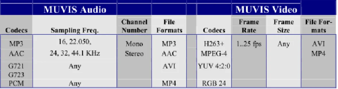
MUVIS databases are formed using the variety of multimedia types belonging to MUVIS multimedia family as given in Table 2-1. The associated MUVIS application will allow the user to create an audio/video MUVIS database in real time via capturing or by converting into any of the specified format within MUVIS multimedia family. Since both audio and video formats are the most popular and widely used formats, a native clip with the supported format can be directly inserted into a MUVIS database without any conversion. This is also true for the images but if the conversion is required by the user anyway, any image can be converted into one of the “Convertible” image types presented in Table 2-2.

(23)

Table 2-1 MUVIS multimedia family

Table 2-2 MUVIS image types

2.3.2. MUVIS Applications

MUVIS applications were firstly developed for Windows OS with specific Win-dows libraries however; those libraries have been integrated to Linux as well. Main fea-tures of the application are presented in the following sections.

DbsEditor deals with indexing and other kind of editing tasks for the MUVIS data-bases. Audio/video clips can be created by a database application as well as available clips could be added to the MUVIS database.

Table 2-2 shows supported formats in the system. On the other hand, different for-mats can be converted and added to the MUVIS database. The fundamental task of DbsEditor is feature extraction. The low-level features are extracted from the image and appended to any given MUVIS database. In addition, DbsEditor is capable of modifying the existing features in a MUVIS database. All the functionalities are presented below.

 Appending and removing multimedia items such as audio/video clips and im-ages

 Dynamic integration and modification of feature extraction (FeX and AFeX) modules.

 Extracting and removing features of multimedia items of a database by using available FeX and AFeX modules.

 Converting of various audio/video files into any MUVIS format

 Preview of multimedia items in a database.

(24)

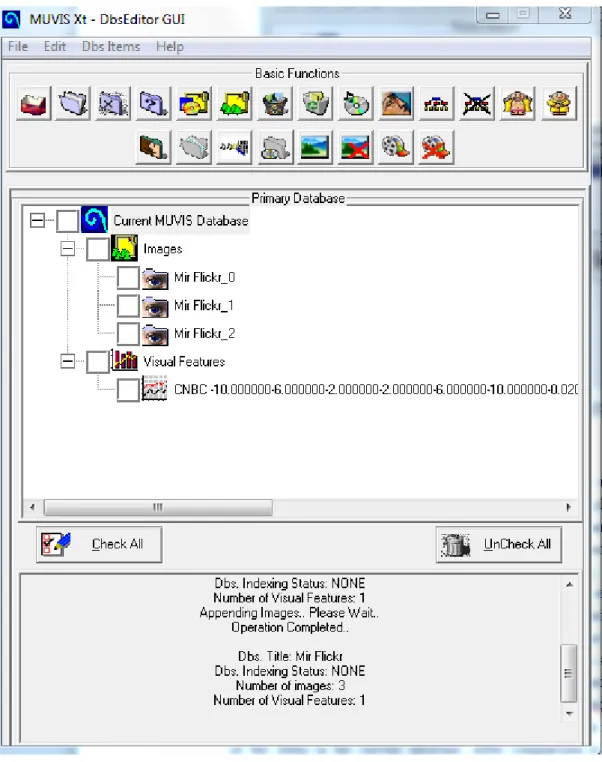
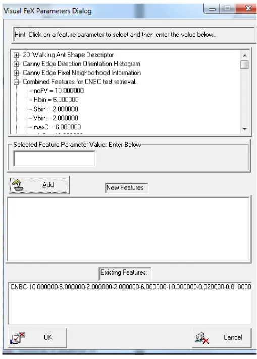
Figure 2-8 demonstrates the interface of DBS Editor. Figure 2-9 is a view of param-eter selection window. Paramparam-eters control the type of feature vectors.

(25)

Figure 2-9 Parameter selection for feature extraction

MBrowser is the skeletal of the application has all the functionalities of a multime-dia player and a robust multimemultime-dia database browser. In addition, users are able to ac-cess any kind of multimedia items in various hierarchic stages. Video display hierarchy is composed of five different levels. These levels are single frame, shot frames (key-frames), scene frames, a video segment and full video clip. MBrowser is implemented with a search and query engine that is able to perform query operation. Query operation is conducted to find the similar multimedia items to the query items. Query image does not need to be in the active database, any kind of external digital image can be used as a query image. The application first appends the query image to the MUVIS database and

(26)

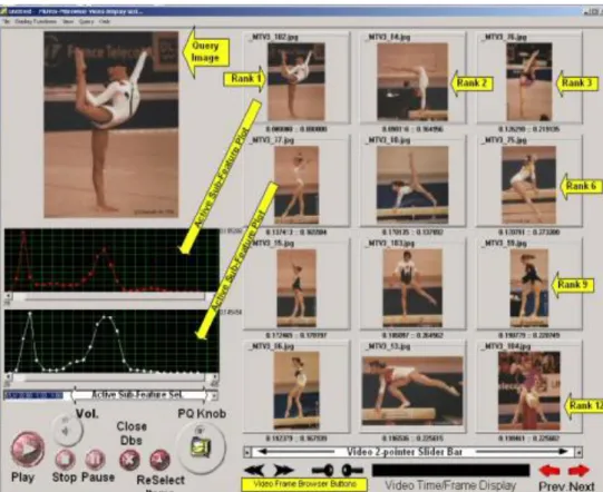
achieves the query operation. Query retrieval is another important component of MBrowser. Retrieval is achieved by comparing the feature vector(s) of the query mul-timedia item with the feature vector(s) of the items in the current database. After com-parison is accomplished, ranking process of similarity distances takes place and pro-gram returns retrieval results for the query primitive. Similarity distance used for rank-ing is measured with special functions implemented separate modules. Progressive Que-ry (PQ) is another attractive method for queQue-ry operation in MBrowser. Normal QueQue-ry (NQ) is the simplest form of query operation that retrieves the total number of matched items. Compared to NQ, PQ is a novel approach for query retrieval. It returns instant query results and allows the user check the preliminary results. Users can stop the query process if they are satisfied with the provided query results. An example PQ approach is shown in Figure 2-10.

Progressive Query approach will be elaborated in the next sub-section.

Summarizing the functionalities of MBrowser, we can use some bullet points.

 Video summarization via scene detection and key-frame browsing,

 Random access support for audio/video clips,

 Displaying any crucial information (i.e. database features, parameters, status, etc.) related with the active database and user commands,

 Visualizations of feature vectors of the images and video key-frames.

 Various browsing options: random, forward/backward and aural or visual HCT (if database is indexed via HCT).

(27)

2.3.3. Indexing and Feature Extraction

DbsEditor, as briefly mentioned in the previous section, performs the indexing of MUVIS databases. The process is achieved in three steps. Database creation is a com-pulsory and first step of the process. This stage deals with sequential indexing that in-dexes (gives a number to each item) the multimedia items in the database. Two optional steps that are used for fast query and Hierarchical Cellular Tree (HCT) browsing func-tionalities follow the first step. The second step deals with feature extraction by means of FeX and AFeX modules. Once features are extracted, the third step performs HCT indexing. Unique characteristics of HCT indexing are as follows.

 Dynamic (Incremental) indexing scheme.

 Parameter invariant (None or minimum parameter dependency)

 Dynamic cell size formation.

 Hierarchic structure with fast indexing (i.e. ~O(nlogn)) formation.

 Similar items are grouped into cells via Mitosis operation(s).

 Optimized for PQ.

Indexing a MUVIS database has a speed advantage. When HCT is used to index a MUVIS database, the similar items can be retrieved faster through “PQ over HCT”. In addition to speed advantage, HCT browsing scheme that is the advanced browsing scheme is activated in MBrowser interface. HCT indexing is not the main requirement for PQ, it is possible to use progressive query with the aid of sequential indexing. Pro-gressive query with sequential indexing is called Sequential ProPro-gressive Query.

MBrowser accommodates two main retrieval schemes for the multimedia items in a MUVIS database: browsing and query-by-example (QBE). In addition to those retrieval schemes, MBrowser provides three different browsing methods: sequential, random and HCT. Indexing is compulsory only for the first two methods. Based on the features in the database as well as the type of the database, visual and aural browsing can be per-formed with HCT browsing. In the cases where both visual and aural features exist in the database, which means the database is hybrid or video database, both of the brows-ing methods can be performed. Nevertheless, for the databases that contain only visual features (i.e. images), only visual HCT browsing is possible.

As shortly mentioned above, two QBE methods are available: Normal Query (NQ) and Progressive Query (PQ). NQ is the basic QBE operation and it utilizes the aural or visual features (or both) of the queried multimedia item (i.e. an image, a video clip, an audio clip, etc.) and all the database items. The algorithm computes the similari-ty distances between feature vectors and then merges them to get a particular similarisimilari-ty distance for each database item to the query item. All the items are ranked according to their similarity distances and the list of the ranked items is the result of the query. NQ has some drawbacks. It is computationally expensive, uses much of the system

(28)

re-sources such as CPU and RAM especially for huge databases. These drawbacks have led us to implement more efficient and robust algorithm for query operation. Thus, Pro-gressive Query (PQ) was born. It is an alternative retrieval approach provides instant sub-results of the query. Therefore, users can interact with the immediate results through MBrowser. MBroswer allows users to browse and control the query operation after the first set of results. Users can stop the query operation if the first set of results is very satisfactory. Eventually, PQ and NQ will return the same set of retrieval results however, PQ is faster than NQ especially if HCT is used to index the database and PQ is performed with HCT.

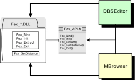
A number of techniques can collect multimedia items. For example, video samples can be captured on real-time and converted to a format that MUVIS recognizes. Once multimedia items are appended to a MUVIS database, their features are extracted and stored in order to accomplish sequential indexing scheme for the database. Visual and aural indexing schemes are achieved with the aid of visual and aural feature extraction frameworks. These modules can be separately implemented as dlls and dynamically integrated to MUVIS system. This mechanism allows developers to integrate third party libraries to the system. Next two paragraphs describe the details of visual and aural fea-ture extraction systems.

Video clips and images provide visual features for a MUVIS database. Features of video clips are extracted from the key-frames of the video clips. During real-time re-cording phase, AVDatabase may optionally and separately store the uncompressed (original) frames of a video clip along with the video bit-stream. If the original key-frames exist, they are utilized feature extraction process. If not, DbsEditor can extract the key-frames from the video bit-stream and use them instead. The key-frames are the INTRA frames in MPEG-4 or H.263 bit-stream. In most cases, a shot detection algo-rithm is used to select the INTRA frames during the encoding stage but sometimes a forced-intra scheme might be present in order to prevent possible degradations. Image features on the other hand are simply extracted from their 24-bit RGB frame buffer, which is obtained by decoding the image.

(29)

Figure 2-11 Interaction of Fex Module with MUVIS applications

The rest of the implementation details of FeX structure are similar to AFeX: each visual FeX module should be implemented as a Dynamic Link Library (DLL) with respect to FeX API, and stored in a suitable directory. FeX API establishes the communication and handshaking between a MUVIS application and the feature extrac-tion module. Figure 2-11 demonstrates the API functions and the basic interaction be-tween MUVIS applications and an illustrative FeX module.

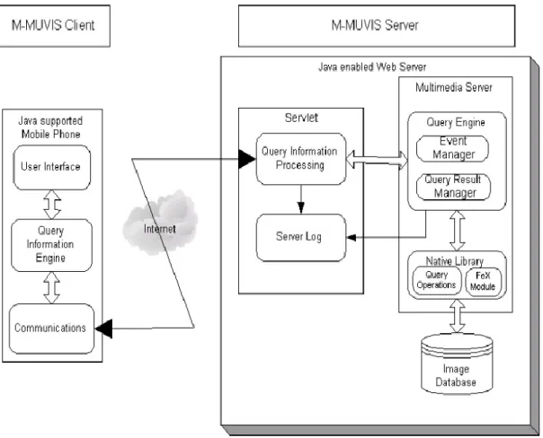
2.3.4. M-MUVIS System

Social media gravitates towards to mobile environment. Google’s CEO Eric Schmidt noted that mobile world is growing faster than their expectations [35]. Nowa-days, mobile phones are faster and more powerful than it used to be. This huge growth renders all PC applications executable in mobile environments. M-MUVIS is a content-based image retrieval system implemented with both Java and C++ [36]. The Image query started by the client application in a mobile device is performed in the server side by means of native C++ code. Query results are sent to the mobile device over network and screened by the user.

M-MUVIS can be divided into two main parts that are client and server side applica-tions. Since the M-MUVIS server have been created using both d native C++ code we can take advantage of scalability, and portability of Java and fast execution of C++ native code. The communication protocol satisfies the criteria of information retrieval most of wireless devices [37].

The client application consists of three components/packages.

a) Query Information Engine: Various data about query are utilized in this engine. This module handles the user activities prepared by user interface in the client device.

b) User Interface: This module handles user interaction with the device such as query operations.

(30)

c) Communication: HTTP [34] protocol is used for the communication over

(GPRS) [38] between device and the server.

Figure 2-12 Demonstration of M-MUVIS system architecture

The essential components of the M-MUVIS server are as follows:

 Native Library

 Query Information Processing

 Server Log

 Query Engine

 Event Manager

 Query Result Manager

The M-MUVIS server accommodates a servlet running inside Java enabled Tomcat web server that contains a database with images that are scaled down to sizes appropri-ate mobile device screens. After query is received, servlet parses and processes it. Que-ry Information Processing module passes the information of the queQue-ry to QueQue-ry Engine and query operation is carried out in Native Library. The query operation can use one or more combination of low-level features . The similarity search is carried out by comparing the feature vectors of query image and the images in the database. After all the similarity distances are computed and ranked, the first 12 images (the most

(31)

simi-lar images to the query image) are retrieved. The simisimi-larity distances are calculated by using the feature vector of queried image with feature vector of the images in a data-base. Ranking operation is performed afterwards and the retrieval result is formed using the best-12 ranked images. Event Manager invokes retrieval result event and Query En-gine sends the retrieval results to Query Information Processing module. The client re-ceives the results as HTTP format and retrieves the images one by one from the server. The query process is demonstrated in Figure 2-13.

Figure 2-13 Query process in M-MUVIS

Even though, M-MUVIS system showed good results, it had some software and hardware limitations, but they are to be solved with the new technological improve-ments such as 3G and smart phones.

(32)

3. SEMANTIC TEXT ANALYSIS USING

WORDNET

3.1. Overview on WordNet and Other Semantic Networks

WordNet is a taxonomy that provides a huge lexical database of English language. Nouns, verbs, adjectives and adverbs are collected into groups of cognitive synonyms (synsets) [3](Miller, 1995)(Miller, 1995)(Miller, 1995). Each synset in the taxonomy corresponds to a gloss that explains the concept of its words. For example the words baby, infant form a synset, this is defined with this gloss in WordNet: a very young child (birth to 1 year) who has not yet begun to walk or talk. Synsets are represented as nodes in WordNet taxonomy and the nodes are linked to each other with a particular relationship. Hyponym indicates that two synsets have is-a-kind-of relation. Meronymy represents is-a-part-of relationship. For example, retriever is a kind of dog and retriever is a hyponym of dog. Antonymy is a opposition relationship such as long-short, female-male.

In our work, we have used WordNet.Net module for semantic similarity measure-ment by Simpson and Dao [39].

3.2. WordNet Based Similarity Measurement

3.2.1. Semantic Similarity between Sentences

Semantic relatedness is a more generic concept than semantic similarity because it also covers antonymy and meronymy relationships. Related concepts are not necessarily similar. For example, female-male are not similar entities but they related in antonymy manner. Relatedness is a more necessary component for most of the applications com-pared to similarity [40].

Semantic similarity measurements calculate the semantic distance between two sen-tences. The output is the confidence score which indicates how similar two documents are, meaning as the score increases the semantic relation increases.

The essential steps for semantic measurement are described in five sections.

 Tokenization

 POS tagging

 Stemming words

 Finding which sense of a word is active in a specific context (Word Sense Dis-ambiguation)

(33)

 Computing the similarity between sentences

Tokenization is theprocess of breaking a set of text up into words, which are called tokens. In addition, stop words that are unimportant words such as article, web pages are eliminated.

Part of speech tagging (POS tagging orPOST) is the process of assigning a part of speech to the words in a text based on its context and definition. POS can be noun, verb, pronoun and adverb. For example, a sentence “John eats an apple” can be decom-posed as John-noun, eats-verb, an-determiner, apple-noun. The tagger algorithm per-forms the tagging with a sentence as input and a specified tag set (a finite list of POS tags) and gives and an output, which is a single best POS tag for each word.

It is worth mentioning two kinds of taggers. Rule-based taggers use hand written rules to disambiguate tag ambiguity, for example Brill's tagger [41]. Stochastic taggers resolve tagging ambiguities by using a training corpus to compute the probability of a given word having a given tag in a given context.

Stemming words is performed with Porter stemming algorithm in order to remove suffixes from words. Terms or words with a common stem mostly have a similar mean-ing, for example:

DEVELOP DEVELOPED DEVELOPING DEVELOPMENT DEVELOPMENTS

Frequently, the performance of an information retrieval system will be improved if term groups such as this are conflated into a single term. This can be achieved by simp-ly removing the suffixes, -ED, -ING, -MENT, -MENTS, to leave the root term DE-VELOP. In addition, the suffix stripping process will reduce the total number of terms in the information retrieval system, and hence reduce the size and complexity of the data in the system, which is always advantageous.

Word Sense Disambiguation identifies the meaning (sense) of a word in a particu-lar sentence. The lexical ambiguity of a word refers to the fact that one word having more than one meaning in the language [42]. Anything can be ambiguous if it is open to more than one interpretation. For instance, consider two instances of the different sens-es of written form of word "spring":

1. Springtime, the season of growth 2. fountain, outflow

and the sentences:

1. I want to stay here until the spring of this year. 2. I like spring water.

(34)

Such situations can lead to some problems while finding the similarity of two words. Humans can distinguish the meaning of words by looking at the context. However, in computational linguistics, word-sense disambiguation (WSD) is a problem of language processing, while finding the meaning used in a sentence, and when the word has multi-ple meanings, which is known as polysemy [42]. A number of supervised approaches have been studied [43], [44], [45]. In addition, a model for WSD is designed based on decision trees using a corpus that consists of 22 million tokens, after manually sense-tagging around 2000 harmonic lines for five test words [46].

Another most commonly used method is the Lesk algorithm [47], which is a dic-tionary-based method. The algorithm is based on the theory that words used in a text stream have semantic relatedness and the relatedness can be determined with the aid of dictionary definitions, so called gloss, of the words. The definitions can also be used to compute the semantic similarity of each pair of word senses in a lexical network such as WordNet.

The main goal is to find the number of words used in common in both glosses. Words overlapping indicate the semantic relatedness of two glosses. For example, [47] performs disambiguation algorithm for the pine cone word pair, the word pine has two senses in the Oxford Advanced Learner's Dictionary,

Sense 1: kind of evergreen tree with needle-shaped leaves, Sense 2: waste away through sorrow or illness.

The word cone has three senses:

Sense 1: solid body which narrows to a point

Sense 2: something of this shape, whether solid or hollow Sense 3: fruit of a certain evergreen tree

Comparing the two senses of the word pine with the three senses of the word cone, evergreen tree can be observed as the most encountered sense for both words. Thus, for the pine cone word pair, Sense 1 of pine is distinguished from the Sense 2 and Sense 3 of cone is distinguished from Sense1 and Sense 2.

In our framework, we used the extended gloss overlap measure algorithm [48] be-cause of the certain constraints of Lesk algorithm.

This algorithm can access a dictionary where adverbs, nouns and adjectives are linked through semantic relations in taxonomy such as WordNet. In this algorithm a better scoring mechanism compared to bag of words counter is used. In the disambigua-tion process, each word in a sentence is considered a target word. The total number of words in a sentence is represented with N. The steps of the algorithm are given below.

(35)

1. Context Selection Context selection is the first step of the algorithm. To reduce the processing time in the cases where N is big, K number of context which is placed in a k-nearest neighbor fash-ion both at the left and right side of the target word is defined. By doing so, we are aim-ing to reduce the computational space and decrease the processaim-ing time accordaim-ingly. For example: If k is six, there will be three words to the left of the target word and three words to the right.

2. Searching words

Searching words is performed to find all possible senses of verbs and nouns in a con-text.

3. Finding Conceptual Relations between Words WordNet provides brief definition for words. These definitions are called gloss. The algorithm seeks the gloss of synonym sets (synset) which are interlinked by means of hyponym, hypernum, mernoym and tropnym.

4. Gloss Pair Combination

In order to measure the relatedness between gloss pairs, overlap of words between two pairs are sought and the overall relatedness score is computed using the separate scores of each pair. The abbreviations stand for comparisons between conceptual relations. For example, measuring the relatedness between two particular sysnsets s1 and s2, the Score(hypo(s1)-hype(s2)) means that the gloss of hyponym of s1 is compared with the gloss of hypernym of s2.

TotalScore(s1,s2)=Score(hype(s1)-hypo(s2))+Score(gloss(s1)-hypo(s2))… (15) In addition, the order of the input does not change the overall score, in other words,

TotalScore(s1,s2) = TotalScore(s2,s1) (16)

The pine cone example above has eighteen possible combinations of senses, six senses for the cone and three for pine. As the scoring mechanism, a new algorithm which distinguishes N-single words from N-consecutive words is used. It also uses glosses as a bag of words. The task is to examine the overlaps between two text streams. The scoring mechanism can be described such that M sequentially overlapping words results M2 units of score, meaning that an overlapping set of words “W X Y Z ” results 42 = 16 units of score whereas “X Y” is 22= 4 and “X Y” +”W Z” is 22+22 =8.

5. After each pair has been successfully scored, the sense which has the highest score is chosen as the most appropriate sense of the target word.

Computing the similarity between sentences is based on the path length between the word senses that are distinguished at the previous step (WSD). Every word sense in WordNet has its own synset, subsequently own node. Similarity between two given sen-tences is computed based on the path-length distance between the synsets.

(36)

entity

object,physical object

vehicle

Natural object

car, auto

automative, motor

artefact

enclosure

_surface

skin

bicycle

Figure 3-1 An example of the hyponym taxonomy in WordNet

In Figure 3-1 the distance between {car, auto} synset and {automotive, motor} synset is 2 while the distance between the concepts in the same synset is 1. The similari-ty score is calculated as follows:

(15) For example, if we are given two sentences A and B where A = {babies drink milk}, B = {Milk is produced from cow}, the algorithm first tokenizes the sentences, thus each word can be processed separately. Then, it performs word stemming and POS tagging to use the words in a dictionary to later perform word sense disambiguation. After the most appropriate word sense, subsequently synset, is computed by WSD a semantic similarity matrix is formed.

3.2.2. Semantic Similarity between Two Synset and Query Sentences

The method explained in the previous section can be considered divide and conquer algorithm since we break down the problem into more sub problems of the same type therefore, it becomes simple enough to be solved. It is used to find the best sense of each word in a given sentence. The semantic similarity between words senses is the main component to find semantic similarity between sentences. Finding the semantic similarity between word senses allows us to find the similarity between sentences.

(37)

The most appropriate senses for the words in a sentence can be extracted using the method explained above. In order to compute the similarity between two sentences, the semantic similarity between word senses is taken into account. Path length is used to measure the similarity between the word senses.

In WordNet hierarchy, if a word has multiple senses, it will be represented in multi-ple synsets in the different parts of the taxonomy. WordNet and records the vari-ous semantic relations between synsets as well as the relations between word senses. The distinction between semantic and lexical relations is crucial. The difference be-tween the semantic relation and lexical relation is that semantic relation describes the relation between two whole synsets while lexical relation describes the relation between words of two different synsets. For example, some semantic relations are hypernym, hyponym, holonym whereas antonym is lexical relations. In WordNet hierarchy, the antonym of the second sense of the noun girl (girl#n#2) is the first sense of the noun boy (boy#n#1). The synset of the noun girl is {girl#n#2, female child#n#1, little girl#n#1}. The antonym of female child#n#1 is male child#n#1.

We have examined three different measurements methods. The first one is path length-based similarity measurement. Each similarity measurement has unique charac-teristics and can be used for different applications.

The path length-based similarity measurement is a popular way of measuring the similarity between nodes. The similarity between synsets is measured based on hypo-nym-hypernym relation, which is also known as is-a relation. However, some limita-tions exist in is-a relation therefore, only two types of POS, noun-noun and verb-verb are used in the framework. Taxonomy is treated as an indirect graph to measure the dis-tance between synsets in WordNet.

In the WordNet noun hierarchy, the term sub sumer refers to a specific shared an-cestor of two concepts (or synsets). The least common sub sumer (LCS) of two concepts is the closest node to them [49]. More particularly, the LCS of two synsets is the most specific sub sumer of the two synsets, which is at the lowest level. In the example above, the LCS of {auto, car} and {truck} is {automotive, motor}, because the {auto-motive, motor} node is the closer node than the common sub sumer which {wheeled vehicle}.

The path length is used to determine the relatedness and the relatedness between concepts is inversely proportional to the path length between two synsets. It other words, the shorter the path length is the more related the words are.

Two synsets of the same part of speech does not need to have a common sub-sumer. However, if a particular ancestor node is used; two synsets will have a connection be-tween each other. In WordNet, synsets are allowed to have more than one ancestor. However, in the cases where a number of paths exist between two synsets, the shortest path is chosen.Lemmatization is done before looking up the word in WordNet. There-fore, the distance between pen and pens is 0, because they are identical. The word worse has bad as its lemma. This link is missed by stemming, as it requires a dictionary look-up. In addition, the word talk is the base form for word talking and henceforth it is

(38)

matched in lemmatization. Different POS are not compared since they are in different taxonomies. Therefore, verbs are compared only with verbs as well as nouns are com-pared only with nouns.

This measurement technique is called MS1 and it has the advantage of being simple to implement and have sufficient performance compared to the other similarity measures such as P. Resnik, Wu and Palmer, Leacock and Chodorow, [50] [51]. Our method can be demonstrated as follows:

Sim(s1,s2) = 1/distance(s1,s2); (16)

where distance is the path length from s1 to s2 using node counting.

The second one is called MS2 and in the method below, the order of the sense is uti-lized in addition to the path.

Sim(s1,s2) = SenseWeight(s1) * SenseWeight(s2)/PathLength (17) where s1 and s2 are the target words that similarity between them is measured. SenseWeight function indicates the ratio of the frequency of the use of input (sense s1) to the frequency of the use of all senses. PathLength, as indicated before, is the node count from s1 to s2.

For the given inputs, the flowchart is illustrated below. For the sentences X and Y, with the lengths m and n respectively, the major steps of finding the similarity can be described as follows:

(39)

Tokenization Stemming POS Tagging Word Sense Disambiguation Score Computation Sentence

Sentence SentenceSentence

Similarity Score

Figure 3-2 The flowchart of semantic similarity between two sentences

Forming a Semantic Similarity Relative Matrix R [m, n] of each pair of word senses at fifth step is quite straightforward. The semantic similarity between the best sense of the word at position i of X and j of Y is represented by R [i, j]. Thus, R [i, j] is also the weight of the edge connecting from i to j. For the words that do not have any gloss in the dictionary, edit-distance similarity is used and it results a lower associated weight. For example, an acronym OSL (Open Source Lab) edit-distance similarity is used. The formula used to capture semantic similarity is a problem of calculating a maximum total matching weight of a bipartite graph. Disjoint nodes are defined as X and Y. In the cas-es where computational time is important, fast heuristic method is used. The pseudo code is given in Table 3-1.