Propulsive Performance in Flapping Locomotion
Thesis by Daegyoum Kim
In Partial Fulfillment of the Requirements for the Degree of
Doctor of Philosophy
California Institute of Technology Pasadena, California
2010
c
⃝ 2010
Acknowledgements
First, I would like to thank Prof. Morteza Gharib, my advisor, for his generous support, which was essential in the completion of this work. His passion and broad interest in research have always motivated me. I was fortunate to do research under his insightful guidance and the great experimental environment he had created.
I extend my thanks to Prof. John Dabiri, Prof. Beverley McKeon and Prof. Dale Pullin for serving on my defense committee and reviewing my dissertation, and Prof. Tim Colonius for serving on my candidacy committee. Their comments were helpful in improving the quality of my work. The discussion with Prof. Fazle Hussain during his visit to Caltech was invaluable in building up my philosophy about academic research. I am also grateful to Prof. Jeff Eldredge whose computational code was a great tool in understanding some of the problems I encountered during my work.
Dr. William Dickson helped me to set up the initial experiment. Without his help, I would have had much more difficulty starting my experiment. I was happy to be with Gharib group members for three years. I gleaned useful information in a variety of fields from them. With the assistance of Martha Salcedo, devoted supporter of our group, I was able to conduct my research without any trouble.
I am grateful to the Samsung Scholarship Foundation for financial aid. Their decision to support me before my application for admission gave me the invaluable opportunity to study at GALCIT.
Abstract
Three-dimensional vortex formation and propulsive performance were studied experimen-tally to identify some of the main characteristic mechanisms of flapping locomotion. Me-chanical models with thin plates were used to simulate flapping and translating motions of animal propulsors. Three-dimensional flow fields were mapped quantitatively using defo-cusing digital particle image velocimetry.
First, vortex structures made by impulsively translating low aspect-ratio plates were studied. The investigation of translating plates with a 90◦ angle of attack is important since it is a fundamental model for a better understanding of drag-based propulsion systems. Rectangular flat-rigid, flexible, and curved-rigid thin plastic plates with the same aspect ratio were used to compare their vortex structures and hydrodynamic forces. The interaction of the tip flow and the nearby vortex is a critical flow phenomenon to distinguish vortex patterns among these three cases. In the flexible plate case, slow development of the vortex structure causes a small initial peak in hydrodynamic force during the acceleration phase. However, after the initial peak, the flexible plate generates large force magnitude comparable to that of the flat-rigid plate case.
sac-rificing total impulse, which is advantageous in avoiding structural failures and stabilizing body motion. The role of the stopping vortex was addressed in optimizing a stroke angle of paddling animals.
In addition, vortex formation of clapping propulsion was investigated by varying as-pect ratio and stroke angle. A low asas-pect-ratio propulsor produces larger total impulse than a high aspect-ratio propulsor. As the aspect ratio increases, circulation of the vor-tex is strengthened, and the inner area enclosed by the vorvor-tex structure tends to enlarge. Moreover, in terms of thrust, the advantage of a single plate over double clapping plates is larger for the lower aspect-ratio case. These results offer information to better understand the benefit of low aspect-ratio wings in force generation under specific locomotion modes. When a pair of plates claps, a vortex loop forms from two counter-rotating tip vortices by a reconnection process. The dynamics of wake structures are dependent on the aspect ratio and the stroke angle.
Vortex formation and vorticity transport processes of translating and rotating plates with a 45◦ angle of attack were investigated as well. In both translating and rotating cases, the spanwise flow over the plate and the vorticity tilting process inside the leading-edge vortex were observed. The distribution of spanwise flow is a prominent distinction between the vortex structures of these two cases. While spanwise flow is confined inside the leading-edge vortex for the translating case, it is widely present over the plate and the wake region of the rotating case. As the Reynolds number decreases, due to the increase in viscosity, leading-edge and tip vortices tend to spread inside the area swept by the rotating plate, which results in lower lift force generation.
Contents
Acknowledgements iii
Abstract iv
1 Introduction 1
1.1 Motivation . . . 1
1.2 Defocusing digital particle image velocimetry . . . 3
1.3 Vortex formation in lift-based and drag-based propulsions . . . 7
1.4 Outline . . . 9
2 Translating motion of rigid and flexible normal plates 11 2.1 Background . . . 11
2.2 Experimental setup . . . 13
2.3 Results and Discussion . . . 16
2.3.1 Vortex formation . . . 16
2.3.2 Effect of tip flow on vortex formation . . . 23
2.3.3 Vorticity transport . . . 26
2.3.4 Correlation between hydrodynamic force and vortex formation . . . 31
2.4 Concluding remarks . . . 34
3 Paddling propulsion 36 3.1 Background . . . 36
3.2 Experimental setup . . . 38
3.2.1 Models and kinematic conditions . . . 38
3.2.2 Defocusing DPIV and force measurement . . . 41
3.3.1 Role of spanwise flow on tip vortex formation . . . 43
3.3.2 Reynolds number dependence of vortex structure and spanwise flow 47 3.3.3 Change of thrust trend by flexible propulsors . . . 50
3.3.4 Optimal stroke angle and vortex shedding . . . 53
3.4 Concluding remarks . . . 57
4 Clapping propulsion 58 4.1 Background . . . 58
4.2 Experimental setup . . . 61
4.3 Results and Discussion . . . 65
4.3.1 Comparison of single-plate and double-plate clapping cases . . . 65
4.3.1.1 Wake dynamics of single-plate cases . . . 65
4.3.1.2 Wake dynamics of double-plate clapping cases . . . 68
4.3.2 Vortex reconnection mechanism in clapping . . . 73
4.3.3 Aspect-ratio effects . . . 77
4.3.3.1 Circulation and impulse . . . 77
4.3.3.2 Wake dynamics . . . 85
4.3.4 Stopping-angle dependence of bound vortex shedding . . . 88
4.3.5 Vortex formation time . . . 90
4.4 Concluding remarks . . . 92
5 Translating and rotating motions with 45◦ angle of attack 94 5.1 Background . . . 94
5.2 Experimental setup . . . 95
5.2.1 Model and kinematic conditions . . . 95
5.2.2 DDPIV process . . . 97
5.2.3 Data analysis . . . 101
5.3 Results and Discussion . . . 102
5.3.1 Comparison between translating and rotating plates . . . 102
5.3.2 Effect of viscosity and velocity program on vortex formation . . . 107
6 Dynamics of corner vortices 114
6.1 Background . . . 114
6.2 Experimental setup . . . 114
6.3 Results and Discussion . . . 116
6.4 Concluding remarks . . . 120
7 Summary and Future work 121 A Scaling of hydrodynamic force by length in 2D translating plates 123 B Validation of approximated vortex moment theory for force calculation 128 B.1 Two-dimensional translating plates . . . 128
B.2 Three-dimensional translating plates . . . 132
List of Figures
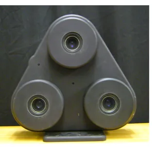
1.1 Front view of the DDPIV camera. . . 3
1.2 Vorticity fields obtained from the DDPIV and the planar DPIV. . . 6
1.3 Circulation of the tip vortex from the DDPIV and the planar DPIV. . . 6
1.4 Vortex structures in lift-based propulsion and drag-based propulsion. . . 8
2.1 Experimental setup. . . 14
2.2 Details of the mechanical model. . . 14
2.3 Shapes of the plates and vortex term definition. . . 17
2.4 Isometric view of the vortex formation process in the flat-rigid plate case. . . 18
2.5 Back view of the vortex formation process in the flat-rigid plate case. . . 18
2.6 Isometric view of the vortex formation process in the flexible plate case. . . . 19
2.7 Back view of the vortex formation process in the flexible plate case. . . 19
2.8 Isometric view of the vortex formation process in the curved-rigid plate case. 20 2.9 Back view of the vortex formation process in the curved-rigid plate case. . . 20
2.10 ωy and ωz distribution at sections in the flat-rigid plate case. . . 21
2.11 Vorticity distribution in front of the plate in the flexible plate case. . . 22
2.12 Close-up to see the vortex deformation in the curved-rigid plate case. . . 22
2.13 Y-directional flow distribution in the flat-rigid plate case. . . 24
2.14 Y-directional flow distribution in the flexible plate and curved-rigid cases. . . 25
2.15 Γy at seven y cross sections in three cases. . . 27
2.16 Vorticity transport rates in the flat-rigid plate case. . . 30
2.17 Drag coefficients of the flat-rigid, flexible, and curved-rigid plate cases. . . 33
2.18 Simple vortex tube representation of figure 2.11 (flexible plate case). . . 34
3.1 Vortex structures in lift-based propulsion and drag-based propulsion. . . 38
3.3 Schematic of the model. . . 40
3.4 Trapezoidal and sinusoidal angular velocity program. . . 40
3.5 Vortex structures for three propulsors with different shapes. . . 44
3.6 Spanwise flow distribution for three propulsors with different shapes. . . 45
3.7 Shape effect on thrust generation for trapezoidal and sinusoidal angular veloc-ity programs. . . 46
3.8 Shape effect on thrust generation for trapezoidal and sinusoidal angular veloc-ity programs. . . 48
3.9 Fence effect of thrust in the delta-shaped plate (EI = 10.9) and trapezoidal velocity program case. . . 49
3.10 Comparison of tip vortex circulation between without-a-fence and with-a-fence cases. . . 49
3.11 Comparison of vortex structures between without-a-fence and with-a-fence cases. 50 3.12 Flexibility effect on thrust generation for four triangular plates with different bending stiffness. . . 51
3.13 Plate shapes for the rigid plate and flexible plate (EI = 1.4) during a power stroke and rotating angle of the plates. . . 52
3.14 Circulation of the tip vortex for the rigid and flexible (EI = 1.4) cases. . . . 53
3.15 Stroke-angle dependence of total impulse for three cases with different shape. 54 3.16 Impulse for five stroke angles in rectangular and delta-shaped plate cases. . . 55
3.17 Formation and shedding of the tip vortex and the corresponding bound vortex. 56 4.1 Experimental setup and details of the model. . . 61
4.2 Notations for angles and definition of a coordinate system. . . 62
4.3 Vortex dynamics in the wake for the AR = 1 andϕ = 45◦ case of single plate. 66 4.4 Vortex dynamics in the wake for the AR = 1 andϕ = 90◦ case of single plate. 67 4.5 Vortex dynamics in the wake for the AR = 1 andϕ= 45◦ case of double plates. 69 4.6 Vortex dynamics in the wake for the AR = 1 andϕ= 90◦ case of double plates. 70 4.7 Circulation Γ andx-directional displacementdxfor the AR = 1 case of double plates. . . 71
4.8 Vortex reconnection process in the AR = 1 and ϕ= 45◦ case. . . 74
4.10 Bound vortex shedding and reconnection in ϕ= 45◦ andϕ= 90◦ cases. . . . 76
4.11 Normal strain rate in the z-direction (duz/dz) on the vortex att= 0. . . 76
4.12 Circulation Γ of the tip vortex at the sections normal to they-axis for single-plate cases att=−0.26 and 0. . . 78
4.13 Velocity distribution on h= 0 section for the ϕ= 45◦ cases. . . 80
4.14 Comparison of vortex structures for single-plate cases. . . 81
4.15 Comparison of tip vortex circulation Γ between single-plate and double-plate cases att= 0. . . 83
4.16 Total impulse I∞ of three different AR cases in various stroke angles. . . 84
4.17 Circulation Γ and x-directional displacement dx of the vortex structure for three AR cases of double plates. . . 85
4.18 Effect of aspect ratio on wake structure at t= 2.09 for double-plate cases (ϕ = 45◦). . . 86
4.19 Second vortex reconnection process for the AR = 2 andϕ= 90◦ case of double plates. . . 87
4.20 Vortex dynamics in the wake for double-plate cases with three different final angles θf. . . 89
5.1 Experimental setup and details of the model. . . 96
5.2 Velocity programs and definition of a coordinate system. . . 98
5.3 Vortex structure by a translating plate of Re = 1100 for t= 0.8∼4.6. . . 103
5.4 Translation case: circulation and vorticity flux at four xy-sections. . . 103
5.5 Translation case: contours of uz on threexy-sections and iso-surfaces ofωx at t = 2.5. . . 104
5.6 Vortex structure by a rotating plate of Re = 1100 for t= 0.8∼4.6. . . 105
5.7 Rotation case: contours of uz on threexy-sections, and iso-surfaces ofωx att = 2.5. . . 105
5.8 Contours ofωx on ayz-section for the translation and rotation cases att= 2.5.106 5.9 Vortex structure by a rotating plate of Re = 8800 and 60 fort= 1.4∼4.6. . 108
5.10 Iso-surfaces of ωz and ωx in Re = 8800 and 60 cases at t= 2.5. . . 108
5.12 Rotation case of the Re = 60 and trapezoidal velocity program: circulation
and vorticity flux at five xy-sections. . . 110
5.13 Rotation cases of the trapezoidal velocity program for Re = 8800 and 1100: circulation at fivexy-sections. . . 111
5.14 Rotation case of the Re = 60 and sinusoidal velocity program: circulation and vorticity flux at five xy-sections. . . 112
6.1 Positions of the model and the camera probe volume inside the tank. . . 115
6.2 Vortex formation process at the corner of the 60◦ corner-angle plate. . . 117
6.3 Vortex formation process at the corner of the 90◦ corner-angle plate. . . 118
6.4 Vortex formation process at the corner of the 120◦ corner-angle plate. . . 119
A.1 Models and kinematic conditions. . . 124
A.2 Force coefficients and circulations for the constant velocity program. . . 125
A.3 Vorticity distribution for the constant velocity program at t= 4.8. . . 125
A.4 Force coefficients and circulations for the sinusoidal velocity program. . . 127
A.5 Vorticity distribution for the sinusoidal velocity program at t= 4.8. . . 127
B.1 Distance between vortex centers. . . 129
B.2 Comparison of impulses calculated from the exact and approximated equations of the vortex moment theory. . . 129
B.3 Comparison of forces calculated from the exact and approximated equations of the vortex moment theory. . . 130
B.4 Comparison of circulations with and without considering vorticity in the bound-ary layer. . . 131
B.5 Comparison of impulses and forces from the approximated vortex moment theory with and without the boundary layer. . . 132
B.6 Comparison of forces from the approximated vortex moment theory and the force transducer measurement. . . 133
C.1 Wing positions of the butterfly during the power stroke for take-off. . . 135
List of Tables
3.1 Summary of the model conditions. . . 41
4.1 Summary of the model conditions. . . 62
4.2 Vortex formation time of the single-plate cases. . . 91
4.3 Vortex formation time of the double-plates cases. . . 92
Chapter 1
Introduction
1.1
Motivation
The study on fluid dynamics of flapping animals has gained attention in recent years be-cause of potential for bio-inspired applications such as micro air vehicles and underwater autonomous vehicles. In addition to the bio-inspired engineering of new propulsion systems, fluid dynamics of animal locomotion has been involved in other multi-disciplinary studies. The unsteady motion of the animal is an attractive model in developing the physics of unsteady flow. Vortex formation by an animal and its relation to propulsive performance is one emerging field of vortex dynamics. In terms of biology, the effects of surrounding fluid on propulsors are also important to understand how the form and function of propul-sors have evolved and been optimized. Moreover, the dynamical interaction of surrounding fluid with sensory and muscular systems is an essential part of understanding locomotive neuronal feedback systems. Furthermore, the structural design of propulsors and its effect on propulsive performance are interesting problems in view of structural mechanics and material science.
problem, researchers have suggested the unsteady lift generation strategies for hovering insects (Ellingtonet al., 1996; Dickinsonet al., 1999). This approach teaches us that a new approach, totally different from the traditional aerodynamic theory, is required in order to understand the principles of flapping locomotion.
In order to better understand the aerodynamics of flying animals, it is also important to find the difference between fixed wings of airplanes and flapping wings of flying animals. First of all, flow around the airplane wing is steady or quasi-steady while flow near the flapping wing is unsteady due to repeated power and recovery strokes. Second, for the fixed wing case, there are specific components responsible for lift, thrust, and control respectively. However, in flying animals, the whole wing is responsible for force production and control without any functional distinction. Third, while airplane wings are rigid and have a high aspect ratio, animal wings are flexible and generally have a low aspect ratio. The effect of flexibility on aerodynamic performance has been studied. The flexible wings of insects are found to be more efficient in lift generation than the stiff wings (Mountcastle & Daniel, 2009; Young et al., 2009). Fourth, for better aerodynamic performance, airplanes and flapping animals use different strategies. flow control (e.g., suppression of flow separation for drag reduction) is important in the fixed-wing aerodynamics to improve the performance. Meanwhile, in flapping animals, the flow is separated from the edge because the angle of attack is relatively high, and optimal vortex formation is the most relevant aerodynamic phenomena in improving their propulsive performance (Dabiri, 2009). The fluid dynamical features of flapping animals mentioned here are also applicable to swimming animals.
Through this thesis work, the primary focus was to study how three-dimensional vortex structures are generated by flapping propulsors under various conditions of kinematics, flexiblity, aspect ratio, and shape of propulsors, as well as the Reynolds number. The Reynolds number studied in this work is in the range of O(10) to O(104). Moreover, the
Figure 1.1: Front view of the DDPIV camera.
1.2
Defocusing digital particle image velocimetry
Here, we briefly explain the DDPIV procedure used in our study. The camera was placed in front of the tank. The tank was filled with water or mineral oil. The tank was seeded with silver-coated glass spheres of mean diameter 100 µm (Conduct-o-fil, Potters Industries Inc.). The particles illuminated by an Nd:YAG laser (200 mJ/pulse, Gemini PIV, New Wave Research Inc.) were captured by the DDPIV camera. The images taken from the DDPIV camera were processed with the DDPIV software based on Pereira & Gharib (2002); Pereira et al. (2006). First, three-dimensional coordinates of the particles inside the tank were found by matching particles in three images captured by the DDPIV camera. Then, from the position information of the particles, the velocity vectors of the particles were calculated from a relaxation method of 3D particle tracking (Pereira et al., 2006). The velocity vectors obtained by this step are randomly spaced in the camera probe volume. The number of cubic grids with size 3 × 3 × 3 mm3 in the mapped domain (about 160 × 160 × 160 mm3) was quite large compared to the number of randomly-spaced velocity vectors obtained from one case (≈5000). To obtain the number of velocity vectors as many as the number of grids, the experiment was repeated 25 (or 20) times under the same conditions with an interval of 90 sec. The interval between the cases was enough to calm the flow generated by the previous case. Then, for each time frame, the randomly-spaced velocity vectors from the 25 (or 20) cases were collected. The collected velocity vectors were interpolated into cubic grids to produce a velocity field. If the number of cases is much more than 25, the accuracy is expected to improve. However, due to a processing time issue, we chose to limit to 25 cases. After removing outlier velocity vectors and applying a smoothing operator to velocity fields, the vorticity field was obtained by a central difference scheme from the velocity data. For smooth rendering of three-dimensional iso-surfaces of vorticity, vorticity vectors were smoothed. The new vorticity at a node was computed byωnew = (ωold+ ¯ωnb)/2 where ¯ωnb is the mean of six neighbor vorticity values. This smoothing process was iterated three times.
For this reason, if the particle is far from the camera, out-of-plane uncertainty of particle coordinates is generally larger than in-plane uncertainty. For the DDPIV system used in this study, the error of the particle position constructed from the images was measured experimentally with the method of Pereira et al.(2000). Inside the camera probe volume, the out-of-plane mean error of the particle position was 40µm for water and 49µm for oil, and the in-plane mean error was 6 µm for both fluids. This error analysis was conducted for the experiment in Ch. 5.
For the validation of the DDPIV, the flow field data obtained by the DDPIV was com-pared to that of the planar DPIV (Willert & Gharib, 1991). The model for Ch. 3 experiment was used for the validation test. The triangular plate was rotated counter-clockwise from the camera view. The Reynolds number based on the mean tip velocity and the span length was 140. The trapezoidal velocity program was used for rotation. For the details of the model conditions and DDPIV procedures, refer to Ch. 3. For image process of the planar DPIV, PIVview2C Ver 3.0 (PIVTEC GmbH) was used. The flow of the symmetrical z= 0 plane was mapped for the planar DPIV. A multi-grid interrogation scheme was used. The first interrogation window size was 96 × 96 pixels with a 50 % overlap, and the final in-terrogation window size was 48 × 48 pixels with a 50 % overlap. The correlation process was repeated twice. The total vectors for each velocity field were 65× 49 vectors. Outlier vectors were removed and replaced by the interpolation from their surrounding neighbor vectors. The grid size of the velocity fields was 4.4×4.4 mm2.
(a) (b)
Figure 1.2: Vorticity fields obtained from (a) the DDPIV and (b) the planar DPIV.
0 0.2 0.4 0.6 0.8 1 1.2 0
0.5 1 1.5
Time t
Circulation
Γ
DDPIV Planar DPIV
1.3
Vortex formation in lift-based and drag-based
propul-sions
The locomotion mechanism of flapping animals can be categorized into two modes: lift-based and drag-lift-based propulsions (Vogel, 2003; Alexander, 2003). In lift-lift-based propulsion, most propulsive force acts perpendicularly to the moving direction of the flapper with a small angle of attack. Meanwhile, in drag-based propulsion with a large angle of attack such as paddling and rowing modes, the propulsive force acts on the flapper mainly in the direction opposite the moving direction of the flapper. Vogel (2003) conjectured that the lift-based propulsion mode was more efficient in high speed locomotion establishing why fast-moving flapping animals employed this mode. He also argued that the drag-based mode was effective in low speed locomotion in that it could generate large thrust over a short time. Therefore, the drag-based propulsion mode is preferred in maneuvering behaviors such as acceleration, turning, and braking (Walker & Westneat, 2000).
The fundamental difference in vortex formation mechanism between lift-based propul-sion and drag-based propulpropul-sion can be understood by examining the relationship between force generation and flow field. The hydrodynamic (aerodynamic) force acting on a moving object inside an infinite flow field can be derived from vorticity distribution of the flow field and velocity of the object (Wu, 1981).
F =−ρf 2
d dt
∫
V∞
x×ωdV +ρf d dt
∫
Vb
udV, (1.1)
whereρf is fluid density,V∞ is an infinite flow field, andVb is body volume. If vorticity is confined in a closed vortex loop of circulation (Γ) and the object is thin, Eq. 1.1 can simply be approximated as follows (Wuet al., 2006),
F(t)≈ −ρf d
dt(ΓS) =−ρf( ˙ΓS+ Γ ˙S). (1.2)
S is the vector of the minimum surface spanned by the vortex loop and |S|is the area of the surface. If propulsive force (Fp) is applied on the object in the negative x-direction,
(a) (b)
Figure 1.4: Vortex structures in (a) lift-based propulsion and (b) drag-based propulsion. The thick green line is the vortex generated by a moving object. The curved arrows around the vortex show the rotating direction of the vortex. The dashed black arrow indicates the moving direction of the object. The thick red arrow indicates the direction of force acting on the object.
1.4
Outline
In the following chapters, translating, padding, clapping, and hovering motions of the plates are examined. The common point of these motions is that the angle of attack is high; either 45◦ for Ch. 5 or 90◦ for the other chapters. Each chapter was written as an independent report. Therefore, some content is duplicated among the chapters. Especially, the procedure explained in the Experimental setup section is quite similar to one another. Here, research topics are outlined.
• Ch. 2 Translating motion of rigid and flexible normal plates
– Effect of flexibility on tip flow and vortex development near the tip.
– Drag force and its correlation with vortex circulation.
• Ch. 3 Paddling propulsion
– Interaction of spanwise flow and a tip vortex and its effect on tip vortex mor-phology.
– Dependence of spanwise flow on plate shape and the Reynolds number.
– Change of thrust trend by flexibility.
– Optimal stroke angle for efficient thrust generation.
• Ch. 4 Clapping propulsion
– Vortex formation and wake dynamics under some stroke angles and aspect ratios.
– Relation between aspect ratios and total impulse.
– Propulsive advantage of double clapping plates over a single plate.
– Formation time for optimal vortex formation.
• Ch. 5 Translating and rotating motions with 45◦ angle of attack
– Comparison of vortex structure and spanwise flow distribution between translat-ing and rotattranslat-ing motions.
– Vorticity transport by convection, tilting and diffusion.
• Ch. 6 Dynamics of corner vortices
Chapter 2
Translating motion of rigid and
flexible normal plates
2.1
Background
The interest in unsteady flow at low to intermediate Reynolds numbers has increased in recent years because of potential bio-inspired applications to micro air vehicles and under-water autonomous vehicles. Previous experimental studies have sought to find the physics of unsteady flow using simple body shapes and simple motions (Dickinson & G¨otz, 1993; Ringuette et al., 2007). Others have used live animals or robotic models to study animal locomotion (Ellingtonet al., 1996; Drucker & Lauder, 1999; Birch & Dickinson, 2001). How-ever, most of these experimental studies were based on two-dimensional flow field measure-ments, which limited their ability to present a complete physical picture of these inherently three-dimensional unsteady flows.
Flapping is a widely used locomotion mode of flying and swimming animals. Propulsion by flapping is used in both air and water in a broad range of Reynolds number regimes (Vo-gel, 2003). The flow induced by the flapping motion of animals has some distinct features. The first feature is the small aspect ratio (AR) of animal wings and fins. Thus, the influence of tip flow is significant. Second, the flow induced by the motion of a flapper is unsteady. Third, the angle of attack of the propulsor can be quite high. Finally, the propulsor is not rigid and has some flexibility in general. In this sense, impulsively starting flexible plates at a high angle of attack in low Reynolds number ranges will be an important model for an in-depth study relevant to animal locomotion.
locomotion since hydrodynamic forces and efficiency are closely related to the generation and transport of vortices. Researchers who have tried to identify vortices in animal loco-motion using flow visualization techniques have pointed to the possible correlation between hydrodynamic force acting on animals and observed vortices (Ellingtonet al., 1996; Drucker & Lauder, 1999; Birch & Dickinson, 2001; Srygley & Thomas, 2002; Speddinget al., 2003). These studies addressed cases where the flapper undergoes complex three-dimensional mo-tion. The lack of a proper three-dimensional flow mapping system as well as the inherent complexity of flow due to three-dimensional motion has posed major difficulties in pro-viding comprehensive principles of flapping motions. Even though it is desirable to study the three-dimensional vortex created by complex flapping motion, we have focused on the vortex structure created in a relatively simple translating motion.
The mechanical properties of the flexible wings of insects and the relation between wing deformation and aerodynamic performance have been studied. Combes & Daniel (2003a) and Combes & Daniel (2003b) measured the bending stiffness of insect wings and found the anisotropy of the bending stiffness in the spanwise and chordwise directions. Combes & Daniel (2003c) insisted that passive wing deformation of their models was mainly caused by inertial-elastic force by rapid acceleration and deceleration, rather than aerodynamic force. From flow visualization, Mountcastle & Daniel (2009); Younget al.(2009) showed that the flexible wings of insects are more efficient in lift generation than the stiff wings. Here, we study the effect of the flexibility on the vortex formation and the trend of force generation. Only the spanwise bending of the plate is considered. By focusing on the translating motion of a rectangular plate, we can isolate the effect of wing flexibility from other effects such as rotation and specific wing geometry.
While many studies have been performed for two-dimensional flow around a translating plate with a high angle of attack as a fundamental study for insect flight (Dickinson & G¨otz, 1993; Pullin & Wang, 2004; Wang, 2004), few have been done for a model with a small AR, either experimentally or computationally, (Ringuetteet al., 2007; Taira & Colonius, 2009). Ringuetteet al.(2007) reported that the unsteady drag coefficient of a plate with a small AR is bigger than the plate with a larger AR because the tip edge contributes to drag. Ringuette
et al.(2007) obtained vorticity fields and calculated the circulation at three sections using
they focused more on the role of the tip vortex in the generation of hydrodynamic force. In order to supplement Ringuette et al.(2007) experiment and find more on the three-dimensional vortex formation process, defocusing digital particle image velocimetry (DDPIV) (Willert & Gharib, 1992; Pereira & Gharib, 2002; Pereiraet al., 2006) was used for the pur-pose of mapping three-dimensional flow fields present in this study. A flat normal plate of AR = 3.75 is translated impulsively in a water tank. In addition, a flexible plate is also used to investigate the effect of plate flexibility on vortex formation and hydrodynamic force generation. A curved-rigid plate, which has a similar shape to the flexible plate at its maximum deformation, is also considered for comparison with the other cases.
2.2
Experimental setup
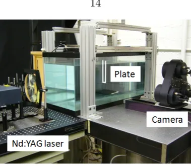
Figure 2.1 shows the experimental setup. A water tank with 870×430×360 mm3
dimen-sions was used for the experiment. Three polycarbonate plates (ρm = 1.2 g/cm3) were used to representflat-rigid,flexible, andcurved-rigid plates. The thickness and Young’s modulus of the rigid plates are 1.52 mm and 2.3 GPa, and those of the flexible plate are 0.25 mm and 2.4 GPa. Even though the plates with 1.52 mm thickness are not completely rigid, the deformation during translation is negligible and, thus, the rigid term is used as a counter-part to the flexible term. The width of the plate was 40 mm. In the middle of the tank, 150 mm of the plate was immersed vertically (figure 2.2). Part of the plate above a free surface was attached firmly to a load cell (miniature beam type, Interface Inc.). A traverse with a lead-screw (Velmex Inc.) to translate the plate was driven by a stepper motor. The traverse accelerated for 0.25 seconds at the start and moved with a constant velocity (Uc) of 50 mm/sec. The Reynolds number based on the constant traverse velocity and plate width (Re =Ucw/ν) was 2000. To make the curved shape for the curved-rigid plate, a hole near a tip edge was penetrated, and the thread was used to connect the hole and the load cell while keeping the plate curved (figure 2.2(b)). We tried to make the curved-rigid plate bend at the same degree as the flexible plate at its maximum deformation. For this purpose, we compared camera images of the curved-rigid and deformed flexible plates. However, there were some deviations in curvatures because it was difficult to match the shapes exactly.
Figure 2.1: Experimental setup. White lines are the edges of the plate model.
(a)
[image:27.595.229.419.56.221.2](b)
volume in the middle of the tank. The tank was seeded with silver-coated glass spheres of mean diameter 100 µm (Conduct-o-fil, Potters Industries Inc.). An Nd:YAG laser (200 mJ/pulse, Gemini PIV, New Wave Research Inc.) was placed to the left side of the camera and optical lenses were used to make a laser cone, which covered the camera probe volume. The traverse system, including the plate model and the load cell, was placed over the tank so that it could be seen from the camera. A stepper motor control computer sent trigger pulses to synchronize the DDPIV camera, the laser, and the motor start. Image pairs were captured at a rate of 5 pairs/sec. The time gap between two laser pulses to take a pair of images was 0.05 sec.
The images taken from the camera were processed with the DDPIV software based on Pereira & Gharib (2002) and Pereiraet al. (2006). First, three-dimensional coordinates of the particles inside the tank were found. Then, from this information, velocity vectors of particles were calculated using a relaxation method of three-dimensional particle tracking (Pereiraet al., 2006). The flow field with 160×160×140 mm3volume was cropped during these processes. The number of cubic grids with size 3×3×3 mm3 in the mapped domain was quite large compared to the number of randomly-spaced velocity vectors obtained from one case. To increase the density of randomly-spaced velocity vectors in a fluid domain, the experiment was repeated 20 times under the same conditions with an interval of 90 sec. For each time step, the randomly-spaced velocity vectors obtained from 20 cases were collected into one and interpolated into cubic grids to produce a velocity field. After removing outlier vectors and applying a smoothing operator to velocity vectors, the vorticity field was obtained by a central difference scheme. For smooth rendering of three-dimensional iso-surfaces of vorticity magnitude, vorticity data were also smoothed. When the plate moved outside of the camera probe volume, the initial position of the plate was moved back 80 mm so that the plate showed up in the camera volume later. Then, another set of the experiment was conducted for the later stage of the plate motion.
force. The same immersed area of the plateS (40 mm×150 mm) and constant velocity of the traverse Uc were used in calculating drag coefficients (CD =D/12ρfUc2S) for all three conditions considered in this study. The drag is the force acting on the plate in the negative x-direction.
Following Gharib et al.(1998), a non-dimensional timeT known asformation time was defined as∫td
0 U(τ)dτ /cwhereU is the traverse velocity,c is the plate width, andtd is the
dimensional time. In figures of§2.3, velocity, vorticity, circulation, and circulation rate are non-dimensionalized;
u= ud Uc
, ω= ωdc Uc
, Γ = Γd Ucc
, Γ =˙ Γ˙d U2
c
, (2.1)
where the subscript dmeans the dimensional variable.
Two non-dimensional parameters are necessary to characterize the problem for the dy-namical interaction of the deformable plate model and the surrounding fluid. Namely,
ρm ρf
= 1.2, EI = (EI)d ρfUc2h3
= 79.8(rigid plate), 0.4(flexible plate) (2.2)
where (EI)dis the dimensional bending stiffness of plates per unit width,ρm andρf are the density of plates and water, and h is the height of the plate inside the tank. Dynamically, the former is the ratio of the inertial force of the deforming plate to the inertial force of the surrounding fluid, and the latter shows the relative magnitude of the bending shear force of the plate over the inertial force of the surrounding fluid.
2.3
Results and Discussion
2.3.1 Vortex formation
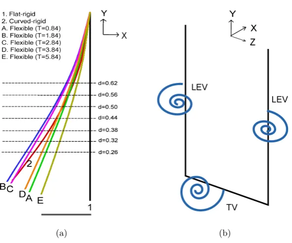
(a) (b)
Figure 2.3: (a) Shapes of the plates immersed in water during traverse movement. The plates are rearranged to have the same base position in order to compare x-directional deviation of the tip from a vertical line. Seven horizontal dashed lines are sections used in
§2.3.3 for Γy calculation. A horizontal continuous line at the bottom is the distance which the traverse travels for ∆T = 1 whereT is the non-dimensional formation time. (b) Vortex term definition. A leading-edge vortex (LEV) is the vortex created along the span. A tip vortex (TV) is the vortex created at the tip.
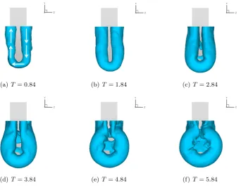
the vortex with the right-hand rule. The regions of lower vorticity, such as the shear layer connecting the vortex core and the boundary layer, are not shown in figures 2.4 to 2.9. The plates shown in these figures are all immersed in water. The top area of the plate is beyond the camera probe volume and, thus, its flow field is absent. Figures 2.4 and 2.5 represent the flat-rigid plate case, figures 2.6 and 2.7 are for the flexible plate case, and figures 2.8 and 2.9 are for the curved-rigid plate case.
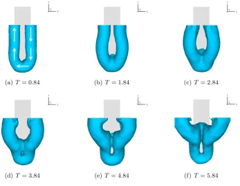
(a) T= 0.84 (b)T = 1.84 (c)T = 2.84
[image:31.595.162.508.56.352.2](d) T = 3.84 (e) T= 4.84 (f) T = 5.84
Figure 2.4: Isometric view of the vortex formation process in the flat-rigid plate case.
(a) T= 0.84 (b)T = 1.84 (c)T = 2.84
(d) T = 3.84 (e) T= 4.84 (f) T = 5.84
[image:31.595.162.510.410.679.2](a) T= 0.84 (b)T = 1.84 (c)T = 2.84
[image:32.595.164.508.54.351.2](d) T = 3.84 (e) T= 4.84 (f) T = 5.84
Figure 2.6: Isometric view of the vortex formation process in the flexible plate case.
(a) T= 0.84 (b)T = 1.84 (c)T = 2.84
(d) T = 3.84 (e) T= 4.84 (f) T = 5.84
[image:32.595.166.510.408.678.2](a) T= 0.84 (b)T = 1.84 (c)T = 2.84
[image:33.595.158.508.57.351.2](d) T = 3.84 (e) T= 4.84 (f) T = 5.84
Figure 2.8: Isometric view of the vortex formation process in the curved-rigid plate case.
(a) T= 0.84 (b)T = 1.84 (c)T = 2.84
(d) T = 3.84 (e) T= 4.84 (f) T = 5.84
[image:33.595.169.512.409.679.2](a)T = 0.84 (b)T = 2.84 (c)T = 4.84
[image:34.595.125.528.65.335.2](d) T = 0.84 (e) T= 2.84 (f) T= 4.84
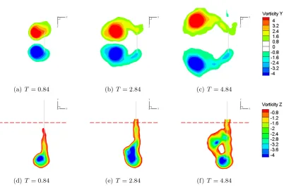
Figure 2.10: ωy and ωz distribution at sections in the flat-rigid plate case. (a)−(c) areωy atT = 0.84,T = 2.84, andT = 4.84. (d)−(f) are ωz atT = 0.84, T = 2.84, andT = 4.84. The height of they-section used for ωy contour is shown as a long dashed line in (d)−(f). z = 0 section (middle section inz-direction) is used for ωz contour.
value of vorticity magnitude is shown in figure 2.10. NearT = 3.84, the TV moves upward continuously due to the tip flow. A similar behavior has been reported by Ringuette et al.
(2007). The upward motion of the TV is concurrent with the tilting of the LEV during the full observation time of the experiment. This continuous upward motion of the TV accentuates the upward propagation of the LEV tilting (figures 2.4(d)−2.4(f)).
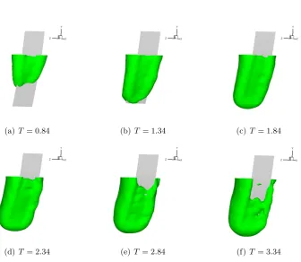
(a) T= 0.84 (b)T = 1.34 (c)T = 1.84
(d) T = 2.34 (e) T= 2.84 (f) T = 3.34
Figure 2.11: Vorticity distribution in front of the plate in the flexible plate case (iso-surface of vorticity magnitude, |ω| = 1.6). Vorticities in front of the upper part tend to move toward the tip.
[image:35.595.164.501.70.362.2](a) (b)
part, the vortex core in the upper part continues to elongate in the x-direction. Note that for the flat-rigid plate case, the LEV in the upper part of the plate moves away from the plate early. However, in the flexible plate case, the LEV in the upper part does not move outward from the plate edge and ends up having an elongated vortex core. When the LEV in the lower part tilts outward to make a horseshoe-shaped vortex, the LEVs in both edges of the upper region show a tendency to move inward. However, the LEV’s inward movement would be limited due to the imposed symmetric condition atz= 0. Instead, the LEV core in the upper part folds and continues to elongate in thex-direction.
For the curved-rigid plate case, the vortex in the lower part of the plate grows faster than that of the flexible plate case. The formation of the vortex into a horseshoe shape in the lower region is more distinct than that of the flexible plate case, and the LEV is tilted vertically in the lower part as is the flexible plate case (figures 2.8(e) and 2.8(f)). The separation of the lower LEV from the plate edge is more distinct than that of the flexible plate case. The vortex system in the lower part of the plate becomes nearly a circular vortex and the vortex core becomes corrugated similar to the flexible plate case. This deformation is concurrent with the severe elongation of the LEV core in the upper part of the plate (figure 2.12).
2.3.2 Effect of tip flow on vortex formation
The outward motion of the LEV is not present in the flow field of impulsively moving two-dimensional flat plates (Koumoutsakos & Shiels, 1996). Thus, it is reasonable to conjecture that three-dimensional effects make the vortex formation process in our cases drastically different from that of their two-dimensional counterpart. The fundamental difference be-tween these two cases is the presence of the tip flow and its influence on the nearby flow field. It will be shown that the main three-dimensional factor for the observed differences is the presence of an upward flow (tip flow in the positive y-direction) near the tip region.
(a)T= 1.84 (b) T = 1.84
(c)T = 3.84 (d) T = 3.84
Figure 2.13: Y-directional flow distribution in the flat-rigid plate case. (a) and (c) are side views of z= 0 section atT = 1.84 and T = 3.84. (b) and (d) are top views of a section at T = 1.84 and T = 3.84, whose y-position is shown in (a) and (c) as a long red dashed line. The contour on the sections is the y-component of the velocity and the three-dimensional transparent surface is the iso-surface of the vorticity magnitude (|ω| = 3.2 for (a) and (c), |ω| = 1.6 for (b) and (d)). Different vorticity magnitudes are chosen to support the explanation in the text better.
move away from the plate, the tip flow gets less entrained by the LEV. Therefore, upward flow becomes more dominant behind the plate, and the TV shifts further up (figures 2.13(c) and 2.13(d)). This observation indicates that upward flow from the tip and its interaction with the LEV has a significant role in early deformation and outward motion of the LEV. In figure 2.13(d), they-component of the velocity,uy, inside the LEV core is negligible, and a high magnitude ofuy is observed near the middle section ofz-direction. In other words, the region of high tip flow does not coincide with the region of vortex cores.
(a)T= 2.84 (b) T = 2.84
(c)T = 4.84 (d) T = 4.84
downward flow in the early stages is the induced flow of the curved vortex that forms along the curved edges of the plates. The direction of flow behind the plate is quite uniform along the curved geometry. It is evident that the entrainment of tip flow by the LEV is not dominant. Therefore, an early separation of the LEV from the plate does not occur in the upper region. Instead, the LEV moves away from the plate first near the lower part where upward tip flow and downward flow meet. This process results in the formation of a vertical horseshoe-shaped vortex near the lower part of the plate. As mentioned in §2.3.1, vortex deformation at the lower region is more apparent in the curved-rigid plate case than in the flexible plate case. Since the LEV of the curved-rigid plate case develops faster than that of the flexible plate after starting, the magnitude of downward flow velocity is larger, which induces more distinct vortex separation from the plate. However, in the flexible plate case, when the plate tip bounces back toward its original position, the tip flow penetrates the region behind the plate. This change of flow pattern may cause a less clear vortex pinch-off process in the lower part of the flexible plate when it is compared to the curved-rigid plate case (figure 2.14).
2.3.3 Vorticity transport
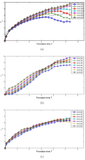
In order to study the vorticity transport of the LEV, first Γy was calculated at several y-sections (figure 2.15). Γy is defined as
∫
A(t)ωydAwhereA(t) is the total area of aycross
0 1 2 3 4 5 6 0
1 2 3 4 5 6
Formation time T
Γy
d=0.26 d=0.32 d=0.38 d=0.44 d=0.50 d=0.56 d=0.62
(a)
(b)
[image:40.595.186.461.83.598.2](c)
For the flat-rigid plate case, Γy grows fast when the plate starts impulsively but is then followed by a gradual decrease in the growth rate. While Γy in the upper part (d≥ 0.50) continues to increase, the growth rate of Γy in the lower part (d ≤ 0.44) becomes almost zero or even negative. Lack of Γy in the lower sections does not mean that the y-component of vorticity,ωy, is not created in the lower part of the plate anymore. Instead, vorticity supplied from the boundary layer in the lower part is lost by convection and tilting processes, which reduce Γy in the lower part. A control volume integral can be used in order to estimate the magnitude ofωy transport. By considering ay cross section in the negative z side as a control surface, we can get the following equation,
d dt
∫
A(t)
ωydA=− ∫
A(t)
uy ∂ωy
∂y dA+ ∫
A(t)
( ωx
∂uy ∂x +ωz
∂uy ∂z
) dA+
∫
L(t)
ν∂ωy
∂n dL (2.3)
the counter-rotating vortex in the other edge should be considered.
Figure 2.16 shows the effect of vorticity transport in the flat-rigid plate case. Threshold values of ωy and uy were applied to obtain the growth rate of Γy by convection or tilting aty-sections;ωy >0.5/sec and|uy|>2 mm/sec. Instead of detailed quantitative analysis, we focus on the characteristics of curves in figure 2.16. While the net vorticity transport is negligible up toT = 1.5, Γy loss by tilting rather than by convection increases considerably in the lower part of the plate after T = 1.5. The upper part does not have any noticeable net vorticity transport during the full observation time in this experiment. When tilting rates atd= 0.26 and 0.34 increase after the lowest peak, tilting rates atd= 0.40 and 0.48 have the lowest peaks in turn. This means a significant tilting motion of the LEV happens from the lower section to the upper section, which is accompanied by the upward motion of the TV. The loss and gain behavior of Γy in figure 2.16 supports the qualitative discussion on the vortex deformation presented in§2.3.1.
(a)
[image:43.595.183.461.189.531.2](b)
2.3.4 Correlation between hydrodynamic force and vortex formation
The hydrodynamic force acting on a body can be obtained from vorticity field data without the need to know the pressure and shear stress on the body. For three-dimensional viscous flow, which rests at infinity, Wu (1981) derived
F =−ρ 2
d dt
∫
V∞
x×ωdV +ρd dt
∫
Vb
udV (2.4)
whereVb andV∞ are body volume and total volume including the body, respectively. In the Euler limit of viscous flow (Re → ∞), added-mass reaction force by linear ac-celeration can be calculated from Eq. 2.4 (Leonard & Roshko, 2001). A solid body can be replaced by the proper vorticity distribution inside the body volume and on the body surface to have the same velocity field in the fluid volume. Then, during acceleration, an incremental velocity ∆Ub of the object proportionally changes the instantaneous strength of the vorticity inside the body volume and on the body surface to satisfy the no-through boundary condition. Therefore, in Eq. 2.4, the first term integrated inside the body volume and on the body surface, as well as the second term, is proportional to dUb/dt. The sum of these two terms is added-mass force. To calculate the total force acting on the body, the first term integrated outside the body volume should be included as well.
If the vorticity is confined in a closed loop of thin vortex filament of circulation Γ, the first term of Eq. 2.4 is reduced to
F =−ρ( ˙ΓS+ Γ ˙S) +ρd dt
∫
Vb
udV (2.5)
qualitative analysis, it is easier to consider one vortex (a collection of vortex filaments), instead of individual vortex filaments. For the vortex of the frontal area Sx and strength Γ, the drag D, the force acting on the plate in the negativex-direction, can be expressed approximately as
D(t)≈ρ( ˙ΓSx+ Γ ˙Sx). (2.6) Growth of vortex strength and frontal area contributes to the drag force. Vortex filaments created on the plate are added to the vortex, which increases the strength of the vortex and contributes to the drag force. The second term of Eq. 2.5 is negligible in our thin plate model with 90◦ angle of attack. During acceleration, the force peak of the second term is much smaller than that of the first term in Eq. 2.4. For the validation of Eq. 2.6 and the effect of the neglected boundary layer on the accuracy of Eq. 2.6, refer to Appendix B.
Figure 2.17 is the graph of the drag measured by the load cell. In the flat-rigid plate and curved-rigid plate cases, drag decreases rapidly after the initial peak and has a plateau after about T = 2.5. The drag of the flat-rigid plate stays higher than that of the curved-rigid plate. For the flexible plate case, the magnitude of the initial peak is not as large as the other cases since only the upper part moves at first. Instead, drag increases again after the initial peak until T = 1 and stays constant during T = 1 ∼ 4. It drops after T = 4 and lies between the drag curves of the other cases. It is interesting to note that the drag of the flexible plate case is comparable to that of the flat-rigid plate case during T = 1∼ 4 even though the plate is curved. If the instantaneous frontal area of the plate is used in the definition of the drag coefficient instead of the immersed area, the drag coefficient of the flexible plate case is higher than that of the flat-rigid plate case duringT = 2∼4; however, the drag coefficient of the curved-rigid plate is not higher than that of the flat-rigid plate even if the instantaneous frontal area of the plate is used.
Figure 2.17: Drag coefficients of the flat-rigid, flexible and curved-rigid plate cases. A continuous line is for the flat-rigid plate; a dashed line is for the flexible plate; a dash-dotted line is for the curved-rigid plate.
vortex frontal surface ( ˙Sx >0) is responsible for the drag plateau (see Eq. 2.6 and figure 2.5). the LEV moves outward in z-direction, which results in positive ˙Sx. However, while the LEV moves outward, some portion of the TV also moves upward to reduce Sx (figure 2.5). Thus, the net effect of the frontal surface change on drag is decreased by the upward TV motion. In the curved-rigid plate case, the circulation slope drops rapidly after starting, and it remains smaller than that of the flat-rigid plate case. AfterT = 3.84, the increase of the vortex frontal surface (figure 2.9) compensates for the decrease of the circulation growth rate, which finally results in nearly constant drag.
X Y
Z
(a)T= 0.84
X Y
Z
(b) T = 3.34
Figure 2.18: Simple vortex tube representation of figure 2.11 (flexible plate case) in the view toward the plate front. While a dark vortex tube is generated from the plate between (a) and (b), a light vortex tube of (a) expands its frontal surface area toward the tip. Arrows indicate the direction of vortices following a right-hand rule. Vortices on the top regions are not shown.
the early formation time, the already-created vortex filaments present for the rigid cases do not contribute to the drag as significantly as the flexible plate case due to their small ˙Sx. However, in the flexible plate case, they can increase the drag force by enlarging their frontal surface area toward the tip. The completion of vortex frontal surface expansion toward the tip may be one of the reasons that the drag value drops afterT = 4. The force trend of the flexible plate case depends on bending stiffness of the plate. Thus, the trend shown in this study cannot be applied to plates with different rigidity without careful investigation.
2.4
Concluding remarks
(upward flow) induces vortex separation and deformation rather than retaining the vortex near the edge of the plate. Unlike the wing of hovering insects, our models undergo only a translating motion and the surface of the model is perpendicular to the moving direction. In this respect, the interaction of the LEV and nearby axial flow depends on the kinematics of the model.
The amount of vortex core deformation is varied by the position of the vortex core and the dynamics of nearby vortex parts. When the vortex can move outward freely after separation from the plate, such as in the upper part of the LEV of the flat-rigid plate case, the vortex core would be able to maintain its original circular shape. In contrast, if the inward motion of the vortex is restricted because of the symmetry condition like the upper part of the LEV of the flexible plate and curved-rigid plate cases, the vortex core would go through severe elongation along the moving direction.
Chapter 3
Paddling propulsion
3.1
Background
The locomotion mechanism of flapping animals can be categorized into two modes: lift-based and drag-lift-based propulsions (Vogel, 2003; Alexander, 2003). In lift-lift-based propulsion, most propulsive force acts perpendicularly to the moving direction of the flapper with a small angle of attack. Meanwhile, in drag-based propulsion with a large angle of attack such as paddling and rowing modes, the propulsive force acts on the flapper mainly in the direction opposite the moving direction of the flapper. Vogel (2003) conjectured that the lift-based propulsion mode was more efficient in high speed locomotion establishing why fast-moving flapping animals employed this mode. He also argued that the drag-based mode was effective in low speed locomotion in that it could generate large thrust over a short time. Therefore, the drag-based propulsion mode is preferred in maneuvering behaviors such as acceleration, turning, and braking (Walker & Westneat, 2000).
process of drag-based propulsion has not been addressed adequately.
Here, we analyze vortex formation and its relation with thrust generation by using a simple mechanical model mimicking the power stroke of drag-based propulsion. In order to map the three-dimensional flow field around our model and identify a vortex structure, defocusing digital particle image velocimetry (DDPIV) was used (Willert & Gharib, 1992; Pereira & Gharib, 2002; Pereiraet al., 2006; Laiet al., 2008). First, we focused on the effect of model shape and flexibility on thrust performance. We also compared flow structures between two different Reynolds number regimes of O(102) and O(104). Furthermore, we explored whether there is an optimal stroke angle for efficient thrust generation and identi-fied flow phenomena that affect the relation between the stroke angle and thrust generation process.
The fundamental difference in vortex formation mechanism between lift-based propul-sion and drag-based propulpropul-sion can be better understood by examining the relationship between force generation and flow field. The hydrodynamic (aerodynamic) force acting on a moving object inside an infinite flow field can be derived from vorticity distribution of the flow field and velocity of the object (Wu, 1981).
F =−ρf 2
d dt
∫
V∞
x×ωdV +ρf d dt
∫
Vb
udV, (3.1)
whereρf is fluid density,V∞ is an infinite flow field, andVb is body volume. If vorticity is confined in a closed vortex loop of circulation (Γ) and the object is thin, Eq. 3.1 can simply be approximated as follows (Wuet al., 2006),
F(t)≈ −ρf d
dt(ΓS) =−ρf( ˙ΓS+ Γ ˙S). (3.2)
S is the vector of the minimum surface spanned by the vortex loop and |S|is the area of the surface. If propulsive force (Fp) is applied on the object in the negative x-direction,
Fp(t) =−Fx(t)≈ρf( ˙ΓSx+ Γ ˙Sx), (3.3)
(a) (b)
Figure 3.1: Vortex structures in (a) lift-based propulsion and (b) drag-based propulsion. The thick green line is the vortex generated by a moving object. The curved arrows around the vortex show the rotating direction of the vortex. The dashed black arrow indicates the moving direction of the object. The thick red arrow indicates the direction of force acting on the object.
generation modes: lift-based propulsion and drag-based propulsion. When a flying animal glides with a constant speed and a small angle of attack (figure 3.1(a)), the circulation of the vortex structure is assumed to be constant in time; the first term ( ˙ΓSx) in the right-hand side of Eq. 3.3 is neglected in lift generation. To apply Eq. 3.3 to drag-based propulsion, we first consider the example of a falling circular disk whose face is perpendicular to the falling direction (figure 3.1(b)). Vorticity is assumed to be created at the edge of the disk and the vortex is rolled up around the edge of the disk. In this case, while the inner area of the vortex loop can be assumed to be approximately constant, the circulation growth of the vortex loop cannot be neglected, and the first term ( ˙ΓSx) of Eq. 3.3 contributes significantly to the lift generation of the falling disk. For drag-based propulsion modes such as paddling and rowing in which the propulsor rotates with a joint, the temporal change of a vortex inner area projected in the thrust direction should also be taken into consideration.
3.2
Experimental setup
3.2.1 Models and kinematic conditions
(a) (b) (c)
Figure 3.2: Shapes of three plates; (a) rectangular plate, (b) triangular plate, and (c) delta-shaped plate for a duck’s feet.
triangle, and delta shape) were considered (figure 3.2). All plates had the same area of 6400 mm2, but the ratio of the plate width in the base to the width in the tip is different. The
delta-shaped plate was chosen to represent the propulsor such as a duck’s foot, which has a much larger area near the tip than near the base. The span lengthsfrom the base to the tip was 160 mm for all plates. The width of the rectangular plate was 40 mm. The widths of the tip and the base in the triangular plate were 65 mm and 15 mm, respectively. The end part of the delta-shaped plate was the equilateral triangle 111 mm wide near the tip. The width of the region connecting the base and the equilateral triangle was 15 mm. The glass plates were assumed rigid. In addition, for flexible plates, transparent polycarbonate plates (Young’s modulus E = 2.3 GPa, density ρm = 1.2 g/cm3) with thickness 1.52 mm, 1.02 mm, and 0.76 mm were used.
(a) Back view (b) Side view
Figure 3.3: Schematic of the model. The plate rotates for a stroke angle ϕwith respect to thez-axis. The rotating axis of the motor is 10 mm above the free surface.
Plate shape Rectangle, triangle, and delta-shape Plate material Glass (thickness 1.15 mm) and
polycarbonate (thickness 1.52 mm, 1.02 mm, and 0.76 mm)
Reynolds number Re 19720 and 140
Angular velocity program Trapezoid and sinusoid
Stroke angle ϕ 106◦
Stroke timeT 2.4 sec
Table 3.1: Summary of the model conditions considered in this study.
140 mm2/sec, ρf = 0.84 g/cm3) for low Re were used as a working fluid inside the tank. The Reynolds number (Re = U s/ν) was 19720 for high Re and 140 for low Re. The span lengthswas used as a characteristic length for Re since our main interest is the tip vortex structure at the tip edge of the plate. The characteristic velocityU for Re is where Ω is the mean angular velocity of the motor during a stroke. In the rigid plate case, U is the same as the mean tip velocity of the plate. In the following sections, the Reynolds number of the model is 19720 unless it is stated specially. The model conditions are summarized in table 3.1.
3.2.2 Defocusing DPIV and force measurement
DDPIV was conducted to map three-dimensional flow generated by a rotating plate. Here, important processing steps are briefly explained. The DDPIV camera was placed in front of the tank. The distance between the camera and the tank was adjusted to place the camera probe volume in the middle of the tank. The tank was seeded with silver-coated glass spheres of mean diameter 100 µm (Conduct-o-fil, Potters Industries Inc.). An Nd:YAG laser (200 mJ/pulse, Gemini PIV, New Wave Research Inc.) illuminated glass sphere particles. The time gap between two laser pulses to take a pair of images was 25 msec. The control computer sent trigger pulses to synchronize operation of the DDPIV camera and the laser, and controlled the stepper motor motion.
the experiment were performed by translating the initial position of the model 80 cm and 160 cm parallel to the tank wall. Thus, the total fluid volume mapped by three sets of the experiment was 280×160×160 mm3. To increase the density of randomly-spaced velocity vectors in a fluid domain, the experiment was repeated 25 times under the same conditions with an interval of 90 sec. For each time frame, the velocity vectors from 25 cases were collected and fitted into grids of 3 × 3 × 3 mm3 to obtain a velocity field. The vorticity field was obtained by a central difference scheme from the velocity field data. The time step between frames was 0.2 sec.
For thrust force measurement, a load cell (miniature beam type, Interface Inc.) was attached to the top of the motor (figure 3.3). The load cell measured the force acting on the plate in thex-direction. The signal was amplified and low-pass filtered with 5 Hz cutoff frequency through a signal conditioner (SGA, Interface Inc.). Thrust coefficient CT and non-dimensional impulseIx were obtained from the filtered signal.
CT(t) =−
Fx(t)
1
2ρfU2ˆr22A
and Ix(t) = ∫t
0CT(τ)dτ
T , (3.4)
where U is sΩ, A is the area of the plate, T is the total stroke time of the plate, and ˆ
r22 is the non-dimensional second moment of plate area with respect to the rotating axis. Non-dimensional total impulseI∞ is the impulse as t goes to∞in Eq. 3.4.
Variables such as time, velocity, vorticity, and circulation were non-dimensionalized with a proper choice of the rotation time T, the span lengths, and the velocity U, which is the mean tip velocity in the rigid plate case;t=td/T,u=ud/U,ω=ωds/U, and Γ = Γd/U s, where a subscriptdmeans a dimensional variable. Matlab (The Mathworks Inc.) was used to obtain circulation (Γd=|
∫
AωzdA|) of the tip vortex at the z = 0 plane. A is the whole
section of the z = 0 plane. The main vorticity component of the tip vortex at the z = 0 plane is negativeωz. To avoid including noise in Γdcalculation, a threshold value ofωz was set;ωz <−0.23.
for flexible polycarbonate plates with thickness 1.52 mm, 1.02 mm, and 0.76 mm in water. This non-dimensional parameter indicates relative magnitude of plate bending shear force with respect to fluid inertial force. Another non-dimensional parameter ρm/ρf represents the ratio of inertial force of the deforming plate to fluid inertial force.
3.3
Results and Discussion
3.3.1 Role of spanwise flow on tip vortex formation
Vortices generated by the power stroke of rectangular, triangular, and delta-shaped glass plates are compared in figure 3.5 for the trapezoidal angular velocity program. One distinct difference among these three cases is the nature of the tip vortex motion. During the stroke, the position of the tip vortex is the lowest along the y-direction in the delta-shaped plate case and the highest in the rectangular plate case. For the delta-shaped plate case, soon after the propulsor starts the power stroke, the tip vortex near the tip edge of the plate separates from the tip edge and moves outward from the tip edge. Meanwhile, the tip vortex for the rectangular plate case relatively follows the trajectory of the tip edge without significant outward motion.
Spanwise flow distribution behind the rotating propulsor is shown in figure 3.6 at t = 0.5 when the propulsor surface is parallel to the y-axis. Spanwise flow is the flow that has the velocity component parallel to the plate span. Outward spanwise flow from the base to the tip is strong and widely distributed for the delta-shaped plate case, compared to the other cases. Spanwise flow occurs mainly in the center region between two side-edge vortex cores. The trends of tip vortex motion and spanwise flow distribution mentioned here were also observed for the sinusoidal angular velocity program cases.
(a) Rectangular plate
(b) Triangular plate
[image:57.595.138.541.153.534.2](c) Delta-shaped plate