Comparisons and Implementation of different Segmentation algorithm based on entropy and energy

Comparisons and Implementation of different

Segmentation algorithm based on entropy and

energy

Mr.Pratik Kumar Dubey1Mr.Naravendra Kumar2Mr. Ajay Suri3 1

M.Tech Sunderdeep Engg. College, Ghaziabad, UP, India 2

Asst.Prof. Sunderdeep Engg. College, Ghaziabad, UP, India 3

HODECE Sunderdeep Engg. College, Ghaziabad, UP, India

Abstract: In image segmentation features like edges, boundaries etc are extracted to characterize images. This emphasizes

the necessity of image segmentation, which divides an image into parts that have strong correlations with objects to reflect

the actual information collected from the real world. Image segmentation is the most practical approach among virtually all

automated image recognition systems. Feature extraction and recognition have numerous applications on

telecommunication, weather forecasting, environment exploration and medical diagnosis. The goal of segmentation is to

simplify and/or change the representation of an image into something that is more meaningful and easier to analyze. Image

segmentation is typically used to locate objects and boundaries (lines, curves, etc) in images. More precisely, image

segmentation is the process of assigning a label to every pixel in an image such that pixels with the same label share certain

visual characteristics. In this paper, there is an algorithm for extracting edges, boundaries from a given image is designed.

For this canny edge detector and Otsu’s method is used. Canny edge detector and otsu method is extracted from image

through image segmentation using different techniques.

Keywords: edge detection, image segmentation, ostu method, canny edge detector.

1. INTRODUCTION

1.1 Introduction to IMAGE Segmentation

Image segmentation refers to partition an image into different

regions that are homogenous with respect to one or several

image features. The process of segmenting an image is easy

to define but difficult to develop.

1.1.1 The Role of Segmentation in Digital Image Processing

Digital images occur very frequently in the world today. All

images on the Internet are in digital form; most images seen in

magazines and newspapers have been in digital form at some

point before publication; and many films have been converted

to a digital format for premastering. Digital Images are

processed simply to improve the quality of the image, or they

may be processed to extract useful information, such as the

position, size or orientation of an object. Image analysis is an

area of image processing that deals with techniques for

this task could be reading an address on a letter or finding

defective parts on an assembly line. More complex image

analysis systems measure quantitative information and use it

to make a sophisticated decision such as trying to find

images with a specified object in an image database. The

various tasks involved in image analysis can be broken down

into conventional (low level) techniques and

knowledge-based (high level) techniques. Image segmentation falls into

the low level category and is usually the first task of any

image analysis process.For example, if the segmentation

algorithm did not partition the image correctly the

recognition and interpretation algorithm would not recognize

the object correctly [1].Over-segmenting an image will

divide an object into different regions. Under segmenting the

image will group various objects into one region. The

segmentation step determines the eventual success or failure

of the image analysis process. For this reason, considerable

care is taken to improve the probability of a successful

segmentation.

1.1.2 The Image

Segmentation:-Image segmentation is an important accepts of the human

visual perception. Segmentation refers to the process of

partitioning a digital image into multiple segments (sets of

pixels, also known as super pixels).Human use their visual

scene to effortlessly partition their surrounding environment

into different object to help recognize their objects, guide

their movements, and for almost every other task in their

lives. It is a complex process that includes many interacting

components that are involved with the analysis of color,

shape, motion and texture of objects. The goal of

segmentation is to simplify and/or change the representation

of an image into something that is more meaningful and

easier to analyze. Image segmentation is typically used to

locate objects and boundaries (lines, curves, etc) in images.

More precisely, image segmentation is the process of assigning

a label to every pixel in an image such that pixels with the

same label share certain visual characteristics. The result of

image segmentation is a set of regions that collectively covers

the entire image, or a set of contours extracted from the image.

Each of the pixels in a region is similar with respect to some

characteristics or computed property, such as colour, intensity,

or texture. Adjacent regions are significantly different with

respect to certain characteristics. Segmentation algorithms

generally are based on one of 2 basis properties of intensity

values. Discontinuity: to partition an image based on abrupt

change in intensity (such as edges).Similarity: to partition an

image into region that is similar according to a set of

predefined criteria [2].

Fig1.1.

1.2 Edge Detection

1.2.1 Edge

An edge is seen at a place where an image has a strong

intensity contrast. Edges could also be represented by a

course there are exceptions where a strong intensity contrast

does not embody an edge. Therefore a zero crossing detector

is also thought of as a feature detector rather than a specific

edge detector.

1.2.2 Edge detection

Edge detection is a very important area in the field of

Computer Vision. Edges define the boundaries between

regions in an image, which helps with segmentation and

object recognition. They can show where shadows fall in an

image or any other distinct change in the intensity of an

image. Edge detection is a fundamental of low-level image

processing and good edges are necessary for higher level

processing. The problem is that in general edge detectors

behave very poorly. While their behavior may fall within

tolerances in specific situations in general edge detectors

have difficulty adapting to different situations. The quality of

edge detection is highly dependent on lighting conditions, the

presence of objects of similar intensity, density of edges in

the scene and the noise. While each of these problems can be

handled by adjusting certain values in the edge detector and

changing the threshold value for what is considered an edge

no good method has been determined for automatically

setting these values, so they must be manually changed by an

operator each time the detector is run with a different set of

data. Since different edge detectors work better under

different conditions, it would be ideal to have an algorithm

that makes use of multiple edge detectors, applying each one

when the scene conditions are most ideal for its method of

detection [3]. In order to create this system, you must first

know which edge detectors perform better under which

conditions. That is the goal of our project. We tested four

edge detectors that use different methods for detecting edges

and compared their results under a variety of situations to

determine which detector was preferable under different set of

conditions. This data could then be used to create multi

edge-detector system, which analyzes the scene and runs the edge

detector best suited for the current set of data.

1.3 Edge Detection Techniques

There are many ways to perform edge detection.

However, the majority of different methods may be grouped

into two categories:

1.3.1 Gradient Techniques

The gradient method detects the edges by looking for the

maximum and minimum in the first derivative of the image.

1.3.2 Laplacian Techniques

The Laplacian method searches for zero crossings in the second

derivative of the image to find edges. An edge has the

one-dimensional shape of a ramp and calculating the derivative of

the image can highlight its location.

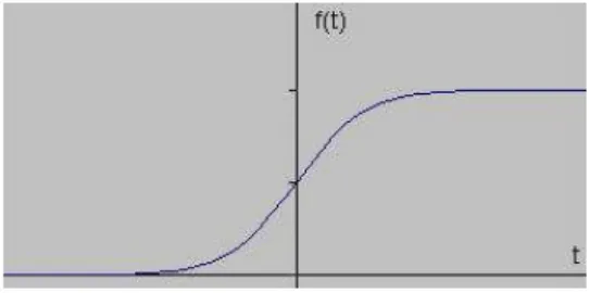
Suppose we have the following signal, with an edge shown by

the jump in intensity below

If we take the gradient of this signal (which, in one

dimension, is just the first derivative with respect to t) we get

the following:

Fig 1.2(b)-First derivative of ramp signal

If we take the gradient of this signal (which, in one

dimension, is just the first derivative with respect to t) we get

the following:Clearly, the derivative shows a maximum

located at the center of the edge in the original signal.

This method of locating an edge is characteristic of the

“gradient filter” family of edge detection filters and includes

the Sobel method. A pixel location is declared an edge

location if the value of the gradient exceeds some threshold.

Edges will have higher pixel intensity clearly; the derivative

shows a maximum located at the center of the edge in the

original signal. This method of locating an edge is

characteristic of the “gradient filter” family of edge detection

filters and includes the Sobel method [4]. A pixel location is

declared an edge location if the value of the gradient exceeds

some threshold. As mentioned before, edges will have higher

pixel intensity values than those surrounding it. So once a

threshold is set, you can compare the gradient value to the

threshold value and detect an edge whenever the threshold is

exceeded. Furthermore, when the first derivative is at a

maximum, the second derivative is zero. As a result, another

alternative to finding the location of an edge is to locate the

zeros in the second derivative. This method is known as the

Laplacian and the second derivative of the signal.

Fig.1.2.C Second derivative of ramp signal

1.3.3 Sobel operator Techniques

The Sobel operator is used in image processing, particularly

within edge detection algorithms. Technically it is a discrete

differentiation operator, computing an approximation of the

gradient of the image intensity function. At each point in the

image, the result of the Sobel operator is either the

corresponding gradient vector or the norm of this vector. The

Sobel operator is based on convolving the image with a small,

separable, and integer valued filter in horizontal and vertical

direction and is therefore relatively inexpensive in terms of

computations. On the other hand, the gradient approximation

which it produces is relatively crude, in particular for high

frequency variations in the image.

In simple terms, the operator calculates the gradient of the

image intensity at each point, giving the direction of the largest

possible increase from light to dark and the rate of change in

that direction. The result therefore shows how "abruptly" or

"smoothly" the image changes at that point and therefore how

as how that edge is likely to be oriented. In practice, the

magnitude (likelihood of an edge) calculation is more

reliable and easier to interpret than the direction calculation.

Mathematically, the gradient of a two each image point a 2D

vector with the components given by the derivatives in the

horizontal and vertical directions. At each image point, the

gradient vector points in the direction of l possible intensity

increase, and the length of the gradient vector corresponds to

the rate of change in that direction. This implies that the

result of the Sobel operator at an image point which is in a

region of constant image intensity is a zero vector and at a

points on an edge is a vecor which points across the edge,

from darker to brighter values [4].

The Sobel Edge Detector uses a simple magnitude. For those

you of mathematically inclined, applying can be represented

as: N(x,y)= ---(1)

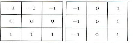
So the Sobel Edge Detector uses two convolution kernels, one to detect changes in vertical contrast (hx) and another to detect horizontal contrast (hy).

Fig 1.3. Sobel masks used for detecting edges

The amazing thing is that this data can now be represented as

a vector (gradient vector).The two gradients computed using

hx and hy can be regarded as the x and y components of the

vector. Therefore we have gradient magnitude and direction.

g= ……… (2)

………. (3)

……….. (4)

Where g is the gradient vector, g is the gradient magnitude and

θ is the gradient direction.

1.3.4 Robert’s Cross Operator Techniques

The Roberts Cross operator performs a simple, quick to

compute, 2-D spatial gradient measurement on an image. Pixel

values at each point in the output represent the estimated

absolute magnitude of the spatial gradient of the input image at

that point. Theoperator consists of a pair of 2×2 convolution

kernels as shown in Figure. One kernel is simply the other

rotated by 90°.

Fig.1.4.Robert mask used for detecting edges

These kernels are designed to respond maximally to edges

running at 45° to the pixel grid, one kernel for each of the two

perpendicular orientations. The kernels can be applied

separately to the input image, to produce separate

measurements of the gradient component in each orientation

(call these Gx and Gy).These can then be 224 combined

together to find the absolute magnitude of the gradient at each

point and the orientation of that gradient.

The gradient magnitude is given

by:-………. (6)

……….. (7)

Which is much faster to compute?

The angle of orientation of the edge giving rise to the spatial

gradient (relative to the pixel grid orientation) is given by:

………. (8)

1.3.5 Prewitt operator Techniques

Prewitt operator is similar to the Sobel operator and is used

for detecting vertical and horizontal edges in images.

Fig 1.5 Prewitt mask used for detecting edges

1.3.6 Laplacian of Gaussian Techniques

The Laplacian is a 2-D isotropic measure of the 2nd spatial

derivative of an image. The Laplacian of an image highlights

regions of rapid intensity change and is therefore often used

for edge detection. The Laplacian is often applied to an

image that has first been smoothed with something

approximately a Gaussian smoothening filter in order to

reduce its sensitivity to noise [5]. The operator normally

takes a single gray level image as input and produces another

gray level image as output.

The Laplacian L(x,y) of an image with pixel intensity value

is given by: ……….(9)

Since the input image is represented as a set of discrete

pixels, we have to find a discrete convolution kernel that can

approximate the second derivatives in the definition of the

Laplacian.

Three commonly used small kernels

Fig 1.6 Laplacian mask used for detecting edges

Because these kernels are approximating a second derivative

measurement on the image they are very sensitive to noise. To

counter this, the image is often Gaussian Smoothed before

applying the Laplacian filter. This post processing step reduces

the high frequency noise components prior to the differential

step. Since the convolution operation is associative we can

convolve the Gaussian smoothing filter with the Laplacian

filter first of all, and then convolve this hybrid filter with the

image to achieve the required result. Doing things this way has

two advantages. Since both the Gaussian and the Laplacian

kernels are usually much smaller than the image, this method

usually requires far fewer arithmetic operations. The LoG

(`Laplacian of Gaussian') kernel can be recalculated in advance

the image. The 2-D LoG function centered on zero and with

Gaussian standard deviation σ has the form

………. (10)

Fig1.7.Laplacian of Gaussian

Note that as the Gaussian is made increasingly narrow, the

LoG kernel becomes the same as the simple Laplacian

kernels shown in Figure. This is because smoothing with a

very narrow Gaussian (σ <.5 pixels) on a discrete grid has no

effect. Hence on a discrete grid, the simple Laplacian can be

seen as a limiting case of the LOG for narrow Gaussians.

1.3.7 Canny edge detector Techniques

Canny’s approach based on three objectives:

1) Low error rate:-All edges should be found and there

should be no spurious responses. i.e. the edges detected must

be as close as possible to the true edges.

2) Edge points should be well localized:-The edges located

must be as close as possible to the true edges. i.e the distance

between a point marked as an edge by the detector and the

center of the true edge should be minimum

3) Single edge point response:-The detector should return

only one point for each true edge point. i.e the number of

local maxima around the true edge should be minimum. This

means that the detector should not identify multiple edge pixels

where only a single edge point exists.

The canny edge detector first smoothes the image to eliminate

gradient to highlight regions with high spatial derivatives. The

algorithm then tracks along these regions and suppresses any

pixel that is not at the maximum (non maximum suppression).

The gradient array is now further reduced by hysteresis.

Hysteresis is used to track along the remaining pixels that have

not been suppressed. Hysteresis uses two thresholds and if the

magnitude is below the first threshold, it is set to zero (made a

non edge). If the magnitude is above the high threshold, it is

made an edge [5]. And if the magnitude is between the 2

thresholds, then it is set to zero unless there is a path from this

pixel to a pixel with a gradient above second threshold.

Fig.1.8. a) Original Image b) Smoothed image c) Non maxima

suppressed image d) Strong edges e) Weak edge f) Final image

2. OSTU METHOD THRESHOLDING

Thresholding is one of the most powerful and important tools

thresholding has the advantages of smaller storage space, fast

processing speed and ease in manipulation compared with

gray level image which usually contains 256 levels. The

thresholding techniques, which can be divided into bi-level

and multilevel category [4]. In bi-level thresholding a

threshold is determined to segment the image into two

brightness regions which correspond to background and

object..Otsu et.al formulates the threshold selection problem

as a discriminate analysis where the gray level histogram of

image is divided into two groups and the threshold is

determined when the variance between the two groups are

the maximum. Even in the case of uni modal histogram

images, that is, the histogram of a gray level image does not

have two obvious peaks, Otsu‘s method can still provide

satisfactory result. In multilevel thresholding more than one

threshold will be determined to segment the image into

certain brightness regions which correspond to one

background and several objects. The selection of a threshold

will affect both the accuracy and the efficiency of the

subsequent analysis of the segmented image. The principal

assumption behind the approach is that the object and the

background can be distinguished by comparing their gray

level values with a suitably selected threshold value. If

background lighting is arranged so as to be fairly uniform,

and the object is rather flat that can be silhouetted against a

contrasting background, segmentation can be achieved

simply by thresholding the image at a particular intensity

level. The simplicity and speed of the thresholding algorithm

make it one of the most widely used algorithms in automated

systems ranging from medical applications to industrial

manufacturing

This method is subject to the following major difficulties:

1. The valley may be so broad that it is difficult to locate a

significant minimum.

2. There may be a number of minima because of the type of

detail in the image, and selecting the most significant one will

be difficult.

3. Noise within the valley may inhibit location of the optimum

position.

4. There may be no clearly visible valley in the distribution

because noise may be excessive or because the background

lighting may vary appreciably over the image.

5. Either of the major peaks in the histogram (usually that dye

to the background) may be much larger than the older, and this

will then bias the position of the minimum.

6. The histogram may be inherently multimodal, making it difficult to determine which the relevant thresholding level is.

3. PROCEDURE FOLLOWED

This method is a nonparametric and unsupervised method of

automatic threshold selection for image segmentation. An

optimal threshold is calculated by the discriminant criterion,

namely, so as to maximize the between-class variance or to

minimize the within-class variance. The method is very simple,

utilizing only the zeroth and first order cumulative moments of

the gray level histogram

Step1-Let the pixels of a given image represented in L gray levels [1;

2; :::; L]. The number of pixels at level i is denoted by ni and

the total number of pixels by N = n1+n2+:::+nL. For

simplification, the gray-level histogram is normalized and

Compute the normalized histogram of the input image.

Denote the components of the histogram by

,i=0, 1, 2…….L-1

Step 2-Compue the cumulative sums, and ,for

k=0,1…L-1

Step 3-Compute the cumulative means m(k) for k=0,1,2L-1

Step 4-Compute the global intensity mean,

Step 5-Compute the between class variance, ,for

k=0,1,2…L-1 using

Step 6-Obtain the Otsu threshold, as the value of k for

which is maximum. If the maximum is not unique,

obtain by averaging the values of k corresponding to the

various maxima detected.

Step 7-Obtain the separability measure, , at k=

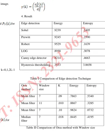
4. Result

Edge detection Energy Entropy

Sobel .9239 .2405

Prewitt .9245 .2390

Robert .9529 .1639

LOG .8958 .3078

Canny edge detector .8214 .4663

Hysteresis thresholding .3533 3.8658

Table I Comparison of Edge detection Technique

Otsu method

Window size

K Energy Entropy

Mean filter 7 .09 .7863 .5340

Mean filter 11 .010 .8867 .3285

Mean filter 7 .10 .9824 .0732

Median filter

7 .018 .8445 .4195

Table II Comparison of Otsu method with Window size

The result shows different segmentation techniques are used

to smoothen an image taking segments of an image. Otsu

method is used to segment an image. Median has lower energy

and therefore is used to smooth the blurred image. Median

filter replaces the value of a pixel by the median of the

intensity levels in the neighborhood of that pixel. Median filter

are effective in the presence of bipolar and unipolar noise. It

shows good result for image corrupted by noise. Mean filter

5. CONCLUSION

The objective is to do the comparison of various edge

detection techniques and analyze the performance of

the various techniques in different conditions. There are

many ways to perform edge detection. The objective function

was designed to achieve the following optimization

constraints maximize the signal to noise ratio to give good

detection. This favors the marking of true positives. Achieve

good localization to accurately mark edges. Minimize the

number of responses to a single edge. This favors’ the

identification of true negatives, that is, non-edges are not

marked The image segmentation allow the user to divides

an image into parts that have strong correlations with objects

to reflect the actual information collected from the real

world. Image segmentation are most practical approaches

among virtually all automated image recognition systems.

Image segmentation is to distinguish objects from images. It

classifies each image pixel to a segment according to the

similarity in a sense of a specific metric distance. To avoid

over-segmentation, foreground and background marker

controlled algorithms are applied with useful outcomes. To

evaluate the roles of both segmentation approaches,

quantitative metrics are proposed rather than qualitative

measures from intuition. Both histograms and to the object

size can be overcome. It is very helpful for the subsequent

processing and improves the success ratio of image

segmentation. Probability distributions are calculated to serve

as the base functions to assess digital images. Using the otsu

method, the problem of its sensitivity

REFERENCES

[1]Zhengmao ye, "objective assessment of Nonlinear Segmentation Approaches to Gray Level Underwater

Images", ICGST-GVIP Journal, pp.39-46, No.2, Vol. 9, April 2009

[2]Rafael C.Gonzalez and Richard E.Woods,”Digital Image Processing”,Third Edition,Pearson Education.

[3]. Wen-Xiong Kang, Qing-Qiang Yang, Run-Peng Liang, "The Comparative Research on Image Segmentation Algorithms," First International Workshop on Education Technology and Computer Science, pp.703-707, , vol. 2, 2009

[4] Jun Zhang and Jinglu Hu, "Image Segmentation Based on 2D Otsu Method with Histogram Analysis", proceedings of International Conference on Computer Science and Software Engineering , IEEE pp. 105-108, 2008.

[5]. Ali Mohammad-Djafari, "A Matlab Program to Calculate the Maximum Entropy Distributions," [Physics-Data-an], Nov. 2001

[6] Qingming haung, wen gao, wenjian cai, ―Thresholding technique with adaptive window selection for uneven lighting image‖, Elsevier, Pattern recognition letters, vol 26, page no 801-808, 2005

[7] M. Sezgin and B. Sankur, “Survey over Image

Thresholding Techniques and Quantitative Performance

Evaluation”, Journal of Electronic Imaging, Vol. 13, pp. 146 -165 , 2004.

[8]N. Otsu, “A Threshold Selection Method from Gray-Level

Histogram”,IEEE Trans. Systems Man, and Cybernetics, Vol.

9, pp. 62-66, 1979.

[9] Tony F. Chan, Member, IEEE, and Luminita A Vese, "Active Contours Without Edges" IEEE Transaction on Image Processing, pp.267-277, No.2,VoLlO, Feb 2001