PERFORMANCE OF SEPARATED RANDOM USER SCHEDULING (SRUS) AND JOUNT USER SCHEDULING (JUS) IN THE LONG TERM EVOLUTION ADVANCED

CLASSIFICATION OF DIABETIC RETINOPATHY PATIENTS

USING SUPPORT VECTOR MACHINES (SVM)

BASED ON DIGITAL RETINAL IMAGE

3_{MUHAMMAD FAISAL,} 2_{DJOKO WAHONO,} 1_{I KETUT EDDY PURNAMA,}

1_{MOCHAMMAD HARIADI,} 1_{MAURIDHI HERY PURNOMO}

1_{Faculty of Industrial Technology Electrical Engineering Department ITS, Surabaya, Indonesia} 2_{Medical Faculty, Brawijaya University, Malang, Indonesia}

3_{State Islamic University of Malang Department of Informatic Engineering, Malang, Indonesia}

E-mail: [email protected], [email protected], [email protected], [email protected]

ABSTRACT

Diabetic retinopathy is a micro vascular complication which is characterized by several changes in the retina. Changes occur in the diameter of the blood vessel, microaneurysm, hemorrhage exudates, and the growth of new blood vessels. These changes need to be detected early so that steps for further handling and treatment can be determined.

Laser therapy is one of the common therapies for patients with Diabetic Retinopathy. This therapy is a manual examination of the scanned results of the fundus retinal image. Manual examinations that generate ophthalmologist sight differ from each other. To overcome this problem, a special program is needed to analyze the fundus image of the eye.

To create a special program for analyzing the fundus images of the eye required several stages of research. The study begins by preprocessing eye fundus images, getting rid of the optic dick form the fundus of the eye and then separating the vascular tissue of the damaged area of the retina. Damaged areas of the retina consist of dark and bright lesians . Mathematical morphology methods are used to detect the presence of dark lesian. To detect the presence of bright lesian a combination of mathematical morphology, Estimated Background, Colour analysis, Max-tree and attribute filters are used by utilizing a branch filtering approach. Fundus image segmentation results are extracted and classified using Support Vector Machines (SVM) based on microneurysm and exudates features. Eye fundus images are classified into, Mild Proliferative Diabetic Retinopathy, Moderate Proliferative Diabetic Retinopathy and Severe Non-Proliferative Diabetic Retinopathy.

The novelty of this research using maxtree representation and atribute filtering to enhance image quality for exudate segmentation.

From the classification experiments on patients with diabetic retinopathy the following sensitivity level were obtained, specificity and AUC above 90%. This indicates that the research could help opthalmologist in analyzing a retina that is affected by diabetic retinopathy. The results of the study showed 96.9% sensitivity, specificity 100%, positive predictive value(ppv) 100%, negative predictive value(npv) 88.19 and AUC 0.985%.

Keywords: Fundus Features, Diabetic Retinopathy, Classification, SVM

1. INTRODUCTION

One of the complications of eye disease caused by diabetes mellitus is diabetic retinopathy. This type of the disease attacks the blood vessels in the retina of the eye, As shown in Figure 1. Affected retina and diabetic retinopathy is the leading cause of blindness in people with diabetes around the world, followed by cataract.

The result of microvascular damage causes pathological changes and cellular dysfunction which can be seen in non-vascular tissue. Early microvascular damage is difficult to explain by circulatory changes [1].

Input Image training

Pre proce ssing

Input Image Testing

Dark Lesion & Bright Lesion Segmentation

using Classification

using SVM Classification Result

Training using SVM

Dark Lesion & Bright Lesion Segmentation

using

Feature Extraction

Pre proce ssing

Figure 2. Research diagram Block

(NPDR) and Proliferative Diabetic Retinopathy (PDR). NPDR is a reflection of clinical hiperpermeabilitas and incompetent blood vessels caused by the blockage and capillary leak. Characteristics of non-proliferative diabetic retinopathy begins with bleeding resulting in microaneurysm, hard exudate, cotton wools, inter retinal microvasculer and venous disorders. Some patients with pathology of diabetic retinopathy need to be diagnosed with diabetes [3]. Besides diabetic retinopathy there are additional symptoms such as hypertensive retinopathy, radiation retinopathy, ocular ischemic syndrome and vascular occlusive disease. This diagnosis is done in order to distinguish the appearance of early symptoms of bleeding points referred to as microaneurysm [4].

Figure 1. Abnormal formations of the retina due to diabetic retinopathy

Manual laser therapy with examination of fundus scanned results is expensive and requires ophthalmologist training [5]. However, manual procedures have some drawbacks because ophtalmologist sight differs from one another.

Several studies of Diabetic retinopathy. The use of filter-based algorithm aimed to get the kernel to recognize microneurysm, where the highest response can be obtained. Generally used filters include multi-scale Gaussian filters [6] and wavelet filters[7].

PV Nageswara rao et al. [8] proposed a new approach for protein classification based on a Probabilistic Neural Network and feature selection

Results of the study [5] that was done regarding exudates segmentation, process of image segmentation using Fuzzy C-Means Clustering by optimizing several clusters. The study was focused on exudates that were not capable of hemorrhages segmentation.

[9] limitations made research on automated detection of exudates by the method of classification of Naive Bayes Classifier. Similarly, [10] to detect retinal damage using K-means Algorithm and Fuzzy C-Means methods.

Giancardo, [11] used a public database HEI-MED dataset for exudate detection using three analysis, namely exudate probability map, color analysis and wavelet analysis. The results showed the presence of some noise that accompanied the analysis of the exudate. Therefore additional research is needed to improve the exudate results. Researchers utilize maxtree and attribute filtering to reduce noise. The problem is corrected in this study by utilizing microneurysm features; exudate is segmented using Max-tree representation and utilizing mathematical morphology.

Furthermore, the extraction of features in each local feature will be selected in advance before it is used for classification. The function of selecting the feature extraction is to select the results that have a large difference between class and ignore the feature extraction results that are not dominant. Selection of these features can be determined using the coefficient of variance.

The next phase is to measure the similarity between the training data and experimental data. One method recently credited as the state of the art in classification is the Support Vector Machine (SVM) [12].

2. MATERIALS AND METHODS

The research data used a combination of eye fundus data from patients at the Malang Eye Clinic, Malang Indonesia.

Research tools used were computers with an Intel Pentium Core (TM) i5-2520M [email protected], 4 GB RAM. Windows 7 Professional operating system, software Matlab.

This section will explain the stages of the research process done to determine what took place in the system. The complete order process can be seen in Figure 2.

Capilar fundus Micro fundus

Microneurysm

2.1. Image preprocessing

2.1.1. Retinal Fundus Image Aquisition

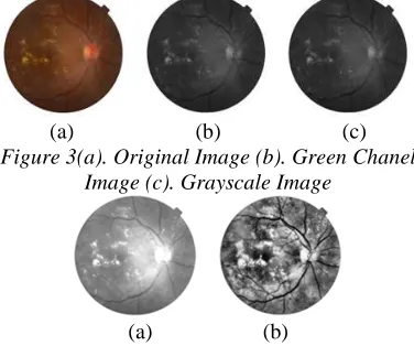
Retinal fundus image aquisition is a process that was first made to include input data in the form of digital retinal fundus image before further processing. The aquisition image is in an RGB image format as shown in Figure 3 (a). To speed up the process of detection, the images were resized to half the size of the original image. Due to the different size of the images, programs are needed to automatically change the image size. The program algorithm is as follows:

1. originalimage size(I);

2. New image [744 round(744*( New image 2)/

New image (1)))];

3. New image New image - mod(New image,2);

4. imgRGB imresize(I, New Image);4.

The size of the original image of the retina fundus from the Eye Clinic Malang is 1416 x 1548, when changed to half of its original size is 708 x 774.

2.1.2. Converting RGB Image to Grayscale Imagery and Green Channel.

The process of converting RGB image into a grayscale image and green channel. Converting image to grayscale to get a bright feature. The process to get dark lesian and entropy values using the conversion to the green image channel. In figure 3 (a) is the fundus input image, Figure 3 (b) is the image of the green channel and Figure 3 (c) is a grayscale image of the fundus. These are carried out to clarify the normalization of objects that exist in the image. The next stage is to increase the contrast of the image using histogram adaptive as shown in figure 4 (a) and 4 (b).

(a) (b) (c)

Figure 3(a). Original Image (b). Green Chanel Image (c). Grayscale Image

(a) (b)

Figure 4(a). Image Contrast (b). CLAHE

2.1.3. Eliminating Blood Vessels in the eye fundus.

The process of eliminating the blood vessels using mathematical morphology. Opening and closing operations. Opening and closing operation is a merger between the operations of erosion and dilation. A dilation operation is done first, followed by the erosion process. This function serves to expand the area were blood vessels are dilated while the erosion function is useful for diluting the blood vessels.

Opening operation of set A by Strel B, expressed as A o B, is defined by:

A o B = (A ϴ _B) ⊕ _{B (1)}

Closing operation of set A by Strel B, expressed as A • B, is defined as:

A • B = (A⊕B) ϴ _{| B (2)}

2.1.4. Optic Disk Detection and Removal In this process, a grayscale image is processed to find the maximum value of each column. Location of optic disk is detected by bright spot on a grayscale image. In order to process, the researcher will make a circle cover which is affixed to the optic disc area (coordinates of the maximum value). The next process is to remove the area covered by the circle, the optical disk will then be removed. The algorithm for automatic detection of the optic disc is as follows:

1. max_GBrigt_column max(G_bright);

2. max_GBright_singlemax(max_GBright_colum

n)

3. [row,column]

find(G_bright==max_GBright_single);

4. med_row floor(med(row));

5. med_column floor(med(column));

6. Radius 90; get area Mask

7. [x,y] meshgrid(1:newSize(2), 1:newSize(1));

8. Mask sqrt( (x - med_column).^2 + (y -

med_row).^2 )<= radius;

2.2. Dark Lesian detection.

the edge of the line (border) to remove the circular border and fill the small covered area. Larger areas will be removed and applied with logic for removing bright lesian (exudate). A dark feature marks the beginning of the microaneurysms. Elimination of exudate is one way of separating light features from dark features.

2.3. Bright Lesian detection

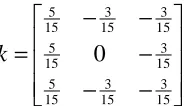
To get a bright area lesion (exudate) the Green Channel Image is converted to HSI. The elimination of a background fundus image using a median filter algorithm [11]. The exudate probability map is used to get the area of the exudate. Exudate were selected using 8-neighbor connected component on Icand. The present study used the edge detection method to get the Kirch's edge exudate. The edge detector is based on the kernel k, with eight different directions above Ig. The equation (3) is as follows:

5 3 3

15 15 15

5 3

15 15

5 3 3

15 15 15

0

k

−

−









=

_

−

_



₋

₋







(3)

Color Analysis utilizes algorithms [13]. This algorithm is explained in that the image is categorized as a scalar mean and standard deviation across all images. By taking a reference image and calculating the parameters of the two categories is more effective than using a simple histogram equalization [11]. The process is as follows:

2

(

)

ref ref ref

I

=

I

−

medianfilter I

Exudate results of the study [11] are corrected to obtain suitable exudates, in the absence of noise it is necessary to have an additional program algorithm. Maxtree and filtering attributes representation were used in research to get the best node.

Results of segmentation methods are represented in tree form. Maxtree algorithm is a raised maxtree proposed by Salembier [14, 15]. In a generated Maxtree, each node will store the information of the flat zone contained therein. This information is an attribute of a flat zone of the node. Information used is leaf, the parent node level, the parent node index, area, child node and child node index level. Information can be obtained from the variable leaf node whether it is a leaf or not. The value of this variable is 0 and 1.

0 indicates that the node stores the information instead of leaf nodes. While 1 indicates that the node is a leaf node.

This information is important for use in the filtering process because the filtering method used is the attribute filtering method, a filtering which is based on information on its leaf node. In parent and child nodes, the information is stored in the form of a gray level image of the parent and the child of the node. Values range from 0 to 255. The variable parent node index and child node index store information from parent and child index of the node. This ranges between 0 to the number of nodes at the parent node level and between 0 to the number of nodes at the level of child nodes. In the area, the information is stored in the form of images of flat zones that are stored on the node.

As mentioned earlier, the generation of image representation is based on the degree of a gray image. The lowest degree of gray will be represented as a root. Child node is a node with a higher degree of gray. Leaf node is a node with the highest degree of gray in a specific region of the image. Formation of Max-Tree can be described as a repetitive or iterative process. In the first iteration, the lowest degree of gray is used as a threshold value h. Then, using the obtained threshold values of pixels that are part of the background and a set of connected components obtained from the pixels with gray level greater than h. Background pixels is then the root node, while the pixels of each connected component will be used to create a temporary storage node. The next iteration is done by the increment threshold value h. With a temporary storage for each node with the degree of gray pixels h to create a new node. Nodes are then added to the tree. Then, a set of connected components are obtained from the pixels with gray levels higher than h. Pixels resulting from every connected component are then placed in the new temporary storage node. Figure 2.6. Illustration shows the process of tree generation Maxtree method.

The next process is the filtering of the tree that has been formed. In the filtering process [14, 15], increasing or non-increasing criteria is used. Each Maxtree node is tested using a predetermined criteria to select the appropriate node and then the node is saved.

are rechecked. This process is repeated until the parent node is found on the lowest determined level. Determination of the lower level is based on the segmentation results using the luca method [11].

The lower limit is used as a base level in the filtering process. So that the filtering process produced some important points that lower level, upper level and lower level parent node. The filtering process produced some important points, namely, the lower level, upper level and parent node in the lower level. From these three points a sub tree can be obtained which is the result of the tree filtering. Image reconstruction of the subtree will result in the fundus images affected by exudate.

Algorithm for maxtree representation and attribute filtering is as follows:

1. f (x , y ) Image

2. mm maxtree ( f (x , y ) ) 3. nn maxgetcount (mm) 4. temp nn

5. temp ( 0 ) 0 6. b i l 0

7. whi l e ( temp ( b i l ) == 0) 8. b i l b i l+1

9. end while

10. lower_ limit b i l 11. top_limit nn (255)

12. for total_node 0 to nn ( top_limit ) 13. parent_l eve l top_limit

14. parent_indeks total_node 15. while ( parent_level > lower_limit )

16. node mmmaxgetnodes (mm,

parent_level , parent_indeks )

17. citra mmmaxsubimage (mm,

parent_level, parent_indeks ) 18. new_image new_image + image 19. parent_level node ( 2 )

20. parent_indeks node ( 3 ) 21. end while

22. end for

23. show(new_image

2.4. Extraction and image classification

Features contain unique information possessed by the image. Features are useful for determining the characteristics of the image for image classification. 5 types of features are used in this research. 2 features are obtained from extractions from the number of pixels on the microneurysm and exudate. 3 features were obtained from statistical extractions value.

Image extraction from microneurysm and exudate is done by counting the number of pixels with the following algorithm,

1. B bwboundaries(area); 2. for area 1:length(B) 3. boundary B( area ); 4. end

5. if isempty(area) 6. area 0;

7. end

For additional extraction value, we use statistical calculations with the equations (5) follows :

∑

=

− = 1

0 ,

)) , ( ln )( , (

N

j i

j i p j i p

Entropy (5)

There are 3 feature of fundus image retrieval entropy value is the value of the green channel gain, the saturation value, RGB value of fundus images.

Features that have been extracted and put into an SVM classification machine for classifying types of normal fundus images and types of fundus image where NPDR is identified.

SVM was first introduced by Vapnik [16]. SVM have shown good performance in data classification. Its success depends on the tuning of several parameters which affect the generalization error [17] . During the early stages classification was limited to only two data classes (binary classification). However, further research developed an SVM that can classify data into more than two classes. There are two options for implementing the multi-class SVM, by combining several binary SVM or combining all of the data which consists of several classes into a form of solving optimization problems. However, the second approach of optimization problem to be solved is much more complicated. This study used a multi-class SVM classification machine which uses a one-against-all method.

One-against-all method is used to construct k, a binary SVM models. (k is the number of classes). Each i classification models are constructed to use the entire data to find solutions to problems, as in equation (6) and equation (7).

0

,

)

.

(

)

.

(

x

x

=

y

x

+

r

y

>

k

is shown in Table 1 and their use in classifying new data can be seen in Table 6.

, ,

1

min

(

)

2

i i j

i T i i

t w b

t

w

w

C

ξ

+

∑

ξ

. (

)

( )

1

,

s t w

φ

x

+ ≥ − → =

b

ξ

y

i

(

w

)

φ

( )

x

+ ≥ − + → ≠

b

1

ξ

y

i

,

ξ

≥

0

Table 1. Example Of 4 SVM With A One-Against-All Method

1

=

i

y yi =−1 Hypothesis

Class 1 Not class 1 f1(x)=(w1)x+b1

Class 2 Not class 2 f2(x)=(w2)x+b2

Class 3 Not class 3 f3(x)=(w3)x+b3

Class 4 Not class 4 f4(x)=(w4)x+b4

3. RESULTS

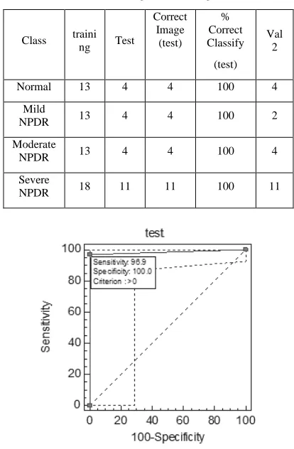
A total of 57 images were extracted to obtain 5 specific features. 57 images consisted of 13 normal eye fundus images; fundus images identified 13 Mild NPDR, identification of mild NPDR in 13 fundus images, identification of moderate NPDR in 13 fundus images and identification of sever NPDR in 18 fundus images. The next step is to calculate the value of true positive (TP), false negative (FN), false positive (FP), true negative (TN). TP shows the image correctly identified as corresponding to the class (positive). FP is an image that should have been identified from the appropriate class classification however there was a mistake in identification TN is the image of the class members, not exactly the class identified (negative). FP indicates that the image should not be a member of the class but is identified as a member of the class. The study can be divided into four classes, namely normal class (positive class), a class that is not normal (negative class), Mild NPDR class (positive class), non-mild NPDR (negative class), Moderate NPDR class (positive class), non-moderate NPDR class (negative class), Severe NPDR class (positive class) and non-sever NPDR (negative class). For more details see Table 6.

Table 2. SVM Biner 4 Class With One-Against-All Method

1

=

i

y yi =−1 Hypothesis

Normal Not Normal f1(x)=(w1)x+b1

Mild NPDR

Non Mild

NPDR

2 2 2

) ( )

(x w x b

f = +

Moderate NPDR

Non Moderate

NPDR

3 3 3

) ( )

(x w x b

f = +

Severe NPDR

Non Severe

NPDR

4 4 4

) ( )

(x w x b

f = +

The ROC classification from 80 digital fundus images showed a sensitivity of 96.9%, spesificity of 100%, positive predictive value (ppv) of 100%, negative predictive value (NPV) of 88.19% and AUC of 0.985. For full results seen Table 7, Table 8 and Figure 5.

Table 3. Training Dan Testing Data

Class traini ng Test

Correct Image

(test) % Correct Classify

(test) Val

2

Normal 13 4 4 100 4

Mild

NPDR 13 4 4 100 2

Moderate

NPDR 13 4 4 100 4

Severe

NPDR 18 11 11 100 11

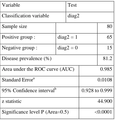
Table 8. Result Of ROC Curve Testing And Validation

Variable Test

Classification variable diag2

Sample size 80

Positive group : diag2 = 1 65

Negative group : diag2 = 0 15

Disease prevalence (%) 81.2

Area under the ROC curve (AUC) 0.985

Standard Errora _0.0108

95% Confidence intervalb 0.928 to 0.999

z statistic 44.900

Significance level P (Area=0.5) <0.0001

4. CONCLUSION

Microneurysm segmentation automatically done by using mathematical morphology is quite effective to obtain its value. Exudate segmentation results are automatically performed by using maxtree and attribute filtering to reduce noise and obtain exudate candidates. This method improved previous researchers methods [11]. Feature extraction using exudate feature values, microneurysm, entropy green channel, green channel homogeneity, the statistical value of saturation images (mean, standard deviation, kurtosis, skewness) can be used a reference for classification.

Performance of Support Vector Machine was in excellent category with a sensitivity value of 96.9%, Spesificity 100%, positive predictive value (ppv) 100%, negative predictive value (NPV) 88.19% and AUC of 0.985.

ACKNOWLEGMENT

Special thanks to Giancardo Luca [11] for supporting author.

REFERENCES:

[1] E. P. Joslin, C. R. Kahn, and G. C. Weir,

Diabetes Mellitus, 14th ed., Boston, Massachusetts: Joslin Diabetes Center, 2006. [2] M. Dharmalingam, “Diabetic retinopathy–

risk factors and strategies in prevention,”

Laser, vol. 51, pp. 77, 2003.

[3] I. M. Stratton, S. J. Aldington, D. J. Taylor et

al., “A Simple Risk Stratification for Time to

Development of Sight-Threatening Diabetic Retinopathy,” Diabetes Care, pp. 1-6, November 12, 2012.

[4] M. Luisa Ribeiro, S. G. Nunes, and J. G. Cunha-Vaz, “Microaneurysm Turnover at the Macula Predicts Risk of Development of Clinically Significant Macular Edema in Persons With Mild Nonproliferative Diabetic Retinopathy,” Diabetes Care, pp. 1-6, November 30, 2012.

[5] A. Sopharak, and B. Uyyanonvara, “Automatic Exudates Detection From Non-Dilated Diabetic Retinopathy Retinal Citra Using Fuzzy C-Means Clustering,” Advances

In Computer Science And Technology, Thailand, 2007.

[6] M. Niemeijer, B. Van Ginneken, M. J. Cree et

al., “Retinopathy Online Challenge: Automatic Detection of Microaneurysms in Digital Color Fundus Photographs ” IEEE

Transactions on Medical Imaging, vol. 29,

2010.

[7] G. Quellec, M. Lamard, P. M. Josselin et al., “Optimal wavelet transform for the detection of microaneurysms in retina photographs,”

IEEE Transactions on Medical Imaging, vol.

9, pp. 1230–1241, 2008.

[8] P. N. Rao, T. U. Devi, D. Kaladhar et al., “A probabilistic neural network approach for protein superfamily classification,” Journal of

Theoretical and Applied Information Technology, vol. 6, no. 1, pp. 101-105, 2009.

[9] A. Sopharak, K. Thet Nwe, Y. Aye Moe et

al., “Automatic Exudate Detection with a

Naive Bayes Classifier,” in The 2008 International Conference on Embedded Systems and Intelligent Technology, Bangkok, Thailand, 2008.

[10] P. Soille, “Morphological Citra Analysis Principles And Application,” Heidelberg,

Springer, 2003.

[11] L. Giancardo, F. Meriaudeau, T. P. Karnowski et al., “Exudate-based diabetic macular edema detection in fundus images using publicly available datasets,” Medical

Image Analysis, vol. 16, pp. 216–226, 2012.

[13] M. J. Cree, E. Gamble, and D. Cornforth, "Colour normalisation to reduce interpatient and intra-patient variability in microaneurysm detection in colour retinal images."

[14] K. E. Purnama, M. H. F. Wilkinson, A. G. Veldhuizen et al., “Branches Filtering Approach for Max-Tree,” University of Groningen, The Netherlands, Groningen, 2007.

[15] M. Faisal, I. K. E. Purnama, M. Hariadi et al., “Retinal blood vessel segmentation in diabetic retinopathy image using maximum tree,” International Journal of Academic

Research, vol. 4, no. 3, 2012.

[16] V. Vapnik, "Statistical Learning Theory", John Wiley & Sons, 1998.

[17] Durgesh K. Srivastava, and L. Bhambhu, “Data Classification Using Support Vector Machine,” Journal of Theoretical and

Applied Information Technology, vol. 12, no.