TIMOC 72 Code Manual EUR 5016

COI

COMMISSION OF THE EUROPEAN COMMUNITIES

TIMOC 72 CODE

DE MANUAL

lAffirø

M

! & '

i','1

■■flëémmw.

mi

.Mafias

m :is¡'.

.¡ÍL*'ÍIMSÍ¡ IÍÍÍVS

ss M i l MlialMraïiii·! ¡ι

Ä l l i Ρ

LEGAL NOTICE

of the Commission ■íà

This document was prepared under the sponsorship of the European Communities.

Neither t h e Commission of the European Communities, its contractors nor any person acting on their behalf:

""•"•Hl· 'reWfi*'tili St jfk# make any w a r r a n t y or representation, express or implied, with respect to the accuracy, completeness, or usefulness of the information contained in this document, or t h a t the use of any information, a p p a r a t u s , method or process disclosed in this document m a y not infringe privately owned rights; or

m

assume any liability with respect to the use of, or for damages resulting from the use of any information, apparatus, method or process disclosed in this document.

%1 tfli"Ι»Αίτ5?* -'\ΜΪΙΛΛ v'iti' " i *íí¿r*in *·

UMÉO

',* _!

_{|*!Ü' HEW}

MJtüJM

•if«*·

^Sü:Wi

This report is on sale a t t h e addresses listed on cover page 4

a t the price of B.Fr. 8 5 , —

C o m m i s s i o n of t h e E u r o p e a n C o m m u n i t i e s D . G . X I I I - C.I.D. 29, rue Aldringen L u x e m b o u r g S e p t e m b e r 1973

USiteí-iii This document was reproduced on the basis of the best available copy.

m

li

l'ÍHi ifP.r'!·

¡Μ

ίαΗΜίΒΜ

Commission of the European Communities

J o i n t Nuclear Research Centre - Ispra Establishment (Italy) Nuclear Study

Luxembourg, September 1973 - 70 Pages - B.Fr. 8 5 . —

T I M O C 72 is a Monte C a r l o Code for the solution of the energy a n d time dependent (or stationary) neutron transport equation in 3-dimensional geometries. I t is an improved version of T I M O C ( H . Kschwendt a n d FL Rief: T I M O C , A general purpose Monte C a r l o code for stationary and time dependent neutron transport, E U R 4519.C, 1970) which is n o w written in F O R T R A N I V IBM-system 360/370. Most of the features described in E U R 4519.e are also incorporated in T I M O C 72. A t present it uses only the very flexible 05R geometry routine, which is able to describe a n y body or body-combination, with surfaces of the 2nd order. A special feature allows the calculation of small perturbation effects. I t is based on the method of similar flight p a t h s a n d on an iteration model to

EUR 5016 e

T I M O C 72 C O D E M A N U A L by R. J A A R S M A a n d FL R I E F

Commission of the European Communities

J o i n t Nuclear Research Centre - Ispra Establishment (Italy) Nuclear Study

Luxembourg, September 1973 - 70 Pages - B.Fr. 8 5 . —

T I M O C 72 is a Monte C a r l o Code for the solution of the energy a n d time dependent (or stationary) neutron transport equation in 3-dimensional geometries. I t is an improved version of T I M O C (FL Kschwendt a n d FL Rief: T I M O C , A general purpose Monte C a r l o code for stationary a n d time dependent neutron transport, E U R 4519.e, 1970) which is n o w written in F O R T R A N I V IBM-system 360/370. Most of the features described in E U R 4519.e are also incorporated in T I M O C 72. A t present it uses only the very flexible 05R geometry routine, which is able to describe a n y body or body-combination, with surfaces of the 2nd order. A special feature allows the calculation of small perturbation effects. I t is based on the method of similar flight p a t h s a n d on an iteration model to

EUR 5016 e

T I M O C 72 C O D E M A N U A L by R. J A A R S M A a n d FL R I E F

Commission of the European Communities

J o i n t Nuclear Research Centre - Ispra Establishment (Italy) Nuclear Study

Luxembourg, September 1973 - 70 Pages - B.Fr. 8 5 . —

approximate an adjoint weighting function as well as the possibility of splitting in the perturbed region. A "tape storage" of the characteristic parameters of neutron histories entering the perturbed region is also possible. This allows the calculation of perturbation effects for different materials w i t h o u t a time consuming recalculation of the w h o l e system. In addition the T I M O C 72 code package contains the program P L O T G E O M . It generates the data for a graphical display of cross sections of the specified geometry b y the C A L C O M P plotter.

approximate an adjoint weighting function as -well as the possibility of splitting in the perturbed region. A "tape storage" of the characteristic parameters of neutron histories entering the perturbed region is also possible. This a l l o w s the calculation of perturbation effects for different materials w i t h o u t a time consuming recalculation of the -whole system. In addition the T I M O C 72 code package contains the program P L O T G E O M . It generates the data for a graphical display of cross sections of the specified geometry by the C A L C O M P plotter.

COMMISSION OF THE EUROPEAN COMMUNITIES

TIMOC 72 CODE MANUAL

by

R. JAARSMA and H. RIEF

1973

Joint Nuclear Research Centre

Ispra Establishment - Italy

ABSTRACT

TIMOC 72 is a Monte Carlo Code for the solution of the energy and time dependent (or stationary) neutron transport equation in 3-dimensional geometries. It is an improved version of TIMOC (H. Kschwendt and H. Rief: TIMOC, A general purpose Monte Carlo code for stationary and time dependent neutron transport, EUR 4519.e, 1970) which is now written in FORTRAN IV IBM-system 360/370. Most of the features described in EUR 4519.e are also incorporated in TIMOC 72. At present it uses only the very flexible 05R geometry routine, which is able to describe any body or body-combination, with surfaces of the 2nd order. A special feature allows the calculation of small perturbation effects. It is based on the method of similar flight paths and on an iteration model to approximate an adjoint weighting function as well as the possibility of splitting in the perturbed region. A "tape storage" of the characteristic parameters of neutron histories entering the perturbed region is also possible. This allows the calculation of perturbation effects for different materials without a time consuming recalculation of the whole system. In addition the TIMOC 72 code package contains the program PLOTGEOM. It generates the data for a graphical display of cross sections of the specified geometry by the CALCOMP plotter.

KEYWORDS

T-CODES P-CODES MONTE CARLO METHOD PLOTTERS

NEUTRON TRANSPORT THEORY CROSS SECTIONS THREE-DIMENSIONAL CALCULATIONS MANUAL

1. INTRODUCTION 5

2. COMPUTER REQUIREMENTS 6

3. PROGRAM ORGANIZATION AND DATA HANDLING 7

4. THE NUCLEAR DATA PREPARATION PROGRAM (1st link) 8

4.1 Input Parameters for the 1st Link Job (NDP) θ

4.2 The Nuclear Data Output 20

5. THE "RANDOM WALK SAMPLING" PROGRAM (2nd link) 21

5.1 Operational Modes and Options (specifications) 21

5.2 Input Data and Formats 23 5.3 Application of the 05R Geometry 29

5.4 The Final Output of Sample Values 31 5.4.1 The Sampling Procedure of Neutron Flux, Current and 31

Angular Flux at Interfaces of Adjacent Regions

5.5 The Re-Run Procedures 37 5.5.1 The Re-Run for Increasing the History number 37

5.5.2 The Re-Run for Performing a Small Effect Calculation 38

6. PLOTGEOM: A PROGRAM FORDISPLAY OF GEOMETRY BY MEANS OF A

CALCOMP PLOTTER 41

6.1 Introduction 41

6.2 Method 41 6.3 Input of the Program PLOTGEOM , 44

6.4 Short Description of the Program 47 6.4.1 Explanation regarding some important subroutines 49

6.5 Description of COMMON and Variables 50

- 4

6.7 Sample Problem 53

6.7.1 Input Data for the Sample Problem 54

6.7.2 Output of the Sample Problem 55 6.7.3 Calcomp output of the Sample Problem 57

6.7.4 Practical example of Calcomp output 58

APPENDICES

Appendix A - Geometry Program 59

1

1. The geometry subroutines GINOUT,GSTRT,GPATH and

GEOPJ 59

2. Modifications in the General 05R Geometry 61

Appendix Β - Random Number Package 63

1. INTRODUCTION *)

This is a report of the FORTRAN IV version of TIMOC ("TIMOC, A General

purpose Monte Carlo code for stationary and time dependent neutron

transport", by H. Kschwendt and H. Rief, EUR 4519e, 1970) originally

written in FAP for use on the IBM 7090/94.

TIMOC 72, as this version is called, uses an improved procedure to

cal-culate small effects. It is based on an iteration model and the

possi-bility of splitting in the "perturbed region". In addition, a different

calculational scheme makes small effect calculations less time consuming

than previously. It will be published elsewhere.

Contrary to the old version, TIMOC 72 uses only the general 05R geometry

routine.

This report deals with the new input description and two sample cases.

The cross section input of the Nuclear Data Preparation Program remains

unchanged, but the specification of the isotope mixtures was simplified.

For all other information the reader should refer to EUR 4519e. The

changes in output are self-explanatory, except those dealing with

the transmission quantities. They are explained in 5.4.1.

2. COMPUTER REQUIREMENTS

TIMOC is a Fortran IV program (IBM system 360) with the exception of

the random number routines. They are a slightly modified version of the

05R package written in the assembler language.

The length of the program depends to a certain extend upon the compiler

option used. The FTH,0 = 2 compiler generates a program of 172 K bytes

to which the length of the two data vectors DV(N) and COMM(M) has to be

added. (Attention: the routine RWSAPR has to be compiled with FTG, since

the FTH,0 = 2 assembly contains an error). These two linear vectors

con-tain most of the nuclear data input, the geometry input and the sampling

values. This length is specified in the main program only. In the present

version of TIMOC the dimensions are DV(20000) and COMM(IOOOO). The

ac-tually required space of the data vectors is part of the print out.

Since COMM(M) is only used during the Data Preparation phase (NDP-step),

DV can in the next step (RWS) be extended into COMM. The available space

3. PROGRAM ORGANIZATION AND DATA HANDLING

A complete computer run of TIMOC 72 consists of two or more steps. The

selection of a step is ruled by certain characters on the title cards

(C0MCA(16), COMCA(17)). In general, the first step will be the Nuclear

Data Preparation performed by the NDP program. The next step is then

the execution of the Random Walk and Sampling (RWS) program.

The RWS program allows the use of several options, described in the

next chapter.

If Small Effects are calculated, i.e. if the SMEC option is used,all

neutron parameters,on the moment of entering into the perturbed regions,

are stored in a data set with the Fortran reference number 11. On Data

set 10 a basic RWS step is completed by writing a Rerun File. This file

can in a RWS-RERUN step be used to augment the number of histories if an

improved statistic is desired.

In the case of Small Effect Calculations in a RWS-SMEC step the Rerun

file on Data set 10 serves together with the SMEC-File on Data set 11 as

8

-4. THE NUCLEAR DATA PREPARATION PROGRAM (1st link)

The Nuclear Data Preparation Program (NDP) searches in the designated

library data set for the required isotopes and prepares the macroscopic

group cross sections, angular distributions, transfer matrices, etc.

re-quired for the Random Walk Sampling problem to be executed afterwards.

The results of this step are written in the data vector DV(J) of blank

COMMON and into the different variables of COMMON/NDRWS/. The NDP program

can be in the computer simultaneously with the RWS program or as the 1st

link of a chain job.

Practical remark: In many cases it is desirable to store the isotope

libraries (i.e.: the microscopic group averaged cross sections usually

prepared by the CODAC code) on a data set (tape) otLer than the

Moni-tor input data set (5).

4.1 Input Parameters for the 1st Link Job (NDP)

CARD COLUMNS FORMAT SYMBOL

1 1 - 6 0 15A4 COMCA(N) =1,15

COMCA(N), N = 1,15: contains the Title identifying the job.

61 1A1 C0MCAQ6)

C0MCA(16) must contain N (or NDP)

67 1A1 C0MCAU7)

C0MCA(17) is either blank if a new problem is treated or

C0MCA(17) is N (or NEWSMEC) if in a perturbed region nuclear

7 - 1 2 13 - 18

16 16

ADDATA INPR

DATSET: Number of Data set containing the cross section libraries and nuclear parameters of the different isotopes.

If DATSET = 5: the cross sections have to be read from the Monitor input data set no. 5, i.e. they follow on cards behind card no. 2.

ADDATA: Allows the input of cross sections on data set 5 in

addi-tion to the ones on the data set specified by DATSET.

IF ADDATA 4 0: the cross sections and nuclear parameters following card no. 2 are used in addition to the ones on data set No. DATSET. If two isotop identifications are identical on data set 5 and DATSET the data on 5 have priority.

INPR: Controls the print out of the cross sections of the speci-fied library.

If INPR ^ 0: all microscopic cross sections and nuclear parameters taken from the library file and used in this computer run are printed.

If INPR = 0: no print out of these data occurs, except for the 3 comment cards (TEXT) preceeding the data of each

iso-tope.

If ADDATA = 0 and DATSET = 5: the following cards 3 to 13

­ 10 ­

CARD COLUMNS FORMAT SYMBOL

If ADDATA = O and DATSET ¿ 5: the following cards 3 to 13

are taken from Data Set No. DATSET (Library Tape).

If ADDATA 4 0 and DATSET Φ 5: cards 3 and 4 are taken from

Data Set 11 and the cards 5 to 13 of Data Set 5 are taken

in addition to the ones of the Library Data Set.

3 1 ­ 6 16 IM

IM: Number of energy groups, not limited.

4 1 ­ 1 1 Ell.4 ENE(I): = 1 , IM + 1.

One card for each number.

ENE(I): The lower energy limits(in eV) of the IM energy groups in increasing

order. ENE(IM+1) = upper limit of the top group. Note that the boundaries

have to be the same for all isotopes. The above set of cards is required

once. The following cards 5) to 13) have to be repeated for each isotope.

All the following nuclear data and group averaged cross sections can be ob­

tained from the ENDF/B data file in the required Formats by the use of the

CODAC code (Ref. 26).

Block I: Parameters which are independent of the energy­group structure

5 1 ­ 6 A6 ISOT Isotope identification

6 3(1­72) 3(12A6) TEXT

CARD 7 COLUMNS 1 7 18 24 35 46 57 - 6 - 17 - 23 - 34 - 45 - 56 - 67 FORMAT A6 Ell.4 16 Ell.4 Ell.4 Ell.4 Ell.4 SYMBOL ISOT ATW IMF FNY AFIS BFIS CFIS

ISOT: Isotope identification

ATW: Atomic weight of the isotope

IMF: Number of different fission spectrum representations to be used (£3)

The energy dependence of the number \T of secondary fission neutrons is

assumed to be described by the following polynomial fitting:

Ό"(Ε) = FNY + AFIS*E + BFIS±E2 + CFIS±E3

E = energy (eV). \

$ (E) can also be given as a group averaged value for each energy group

separately, see card 9.

1 7 18 29 40 51 - 6 - 17 - 28 - 39 - 50 - 61 16 Ell.4 Ell.4 Ell.4 Ell.4 Ell.4 LTT EMIN EMAX ELCO(l) ELC0(2) ELC0(3)

LTT: Symbol defining type of fission spectrum

EMIN, EMAY: Lower and upper limit (in eV) for the corresponding

- 12

CARD COLUMNS FORMAT SYMBOL

ELCO(l): A

ELCO(2): Β

ELCO(3): C

LTT = 6 or 7: Simple fission spectrum

X(E)

=

BfFexp(-E/A)

LTT = 8 or 9: Maxwellian distribution

1(E)-

B-E-exp(-g

LTT = 10: Watt spectrum

X(ihC-exp(-E/A)'Sinh(fOT)

There can be a maximum of 3 cards of type 0 per isotope,

Block II: All microscopic group averaged cross sections split into the

capture, elastic scattering, inelastic scattering and fission parts and

(optional) the particle multiplication factor for fission.

1

7

18

29

40

51

62

- 6

- 17

- 28

- 39

- 50

- 61

- 72

A6

Ell.4

Ell.4

Ell.4

Ell.4

Ell.4

Ell.4

ISOT

ENCH

CROM(l)

CR0M(2)

CR0M(3)

CR0M(4)

CR0M(5)

ISOT: Isotope identification

CARD COLUMNS FORMAT SYMBOL

CROM(l): is l» , the microscopic capture cross section ­24 2

Unit: barn (= 10 cm ) .

CR0M(2): is (J1,T , the microscopic elastic scattering cross section

Γι il

Unit: barn.

CR0M(3): is ^XN> t n e microscopic inelastic scattering cross section

Unit: barn.

CR0M(4): is C^T» the microscopic fission cross section

Unit: barn.

CR0M(5): is >J (like on card 7 ) . If CR0M(5) ¿ 0, this value is taken for

the determination of the product ^ 0 r I

Block III: All information on elastic isotropic or anisotropic scattering

A card 10 must be present for each energy group (in increasing order) in

which G" 4 0. If required, card 10 must be followed by the corresponding

till

card 11. The card(s) describe(s) the differential cross sections for the

elastic anisotropic scattering.

10 1

7

18

24 ­ 6

­ 17

­ 23

­ 29

A6

Ell.4

16

16

ISOT

ENCH

LTT

NE

ISOT: Isotope identification

ENCH: Lower boundary of the energy group (eV)

LTT: Symbol defining angular distribution description

­ 14 ­

CARD COLUMNS FORMAT SYMBOL

LTT = ­1: The same angular distribution function as in the previous group

is used. Card 11 must be omitted.

LTT = 0: Isotropic scattering distribution in the c m . system. Card 11

must be omitted.

LTT = 1: The distribution is described by a Legendre polynomial in the

c m . system. The program expects on card 11 NE Legendre coeffi­

cients for the anisotropic distribution.

NE­1

¡¿^=yELCO(n

l)-P

(cos#)

LTT = 2: Anisotropic scattering is described in the c m . system by a poly­

gon. NE is the number of equidistant points along the ¿^­axis in

the d fc/å Li table ( £ 40) .

Ψ

LTT = 3: The averaged value cos θ of the angular distribution in the lab.

system is used.

Card(s) 11 must only be given, if LTT^l.

11 1 ­ 1 1 Ell.4 ELC0(1)

ELC0(I),I = 1,HE

• * ·

56 ­ 66 Ell.4 ELC0(6)

etc.

CARD COLUMNS FORMAT SYMBOL

If LTT = 2: The ELCO(I) are the NE values (< 40) of the angular distribution

d<?Vd μ at equidistant points between [+1, -li , including the boundaries.

The number of intervals is therefore NE-l. The ELCO(I) must be given for the

distribution in the c m . system and in decreasing order of cos V I +1-> -1 / .

Note that in each group another type of anisotropic scattering may be used.

Block IV: All information on inelastic scattering and transfer matrices

12 1 - 6

7 - 1 7 18 - 23 24 - 29

A6 Ell.4 16 16

ISOT ENCH LTT NU

ISOT: Isotope identification

LTT defines the inelastic scattering description

ENCH: Lower energy boundary

NU: Number of parameters following on card 13

LTT = -1: The same scattering values are used as in the previous energy group.

LTT = 1: The model of excited levels is used.

LTT = 2: The statistical model is used.

LTT = 3: Energy transfer is described by a transfer matrix.

Card 13 must be given if LTT^l.

If LTT = 1 or 2 card 13 reads like

13 1 - 1 1 Ell.4 ELCO(l)

ELC0(1),I = 1,NU

­ 16 ­

a) For LTT = 1 and NU ^ 2 (excited level description) this means:

ELCO(l): <u E for first energy level ( Δ E is negative for down scattering)

ELC0(2): Partial probability for first level

ELC0(3): & E for second level and so on until NU values have been read in.

The partial probabilities are normalized by the program and the

sum does not have to agree with the total inelastic cross section.

Since in most calculations discrete energy values appear during

the course of a history it can happen that in some energy group

the subtraction of J E leads to a negative value of the energy

after the collision. If E ­ à E¿ 0, for E.+,¿ E¿E. , the program

chooses another level (if possible) or an elastic collision pro­

CARD COLUMNS FORMAT SYMBOL

b) For LTT = 2 and NU = 1 (statistical model (ELCO(l)) is the nuclear

temperature for the group under consideration.

c) If LTT = 3 and NU ~γ 3 (transfer matrix version in this energy group)

13

7 - 1 7 Ell.4 18 - 28 Ell.4

ELCO(I),I = 1,NU 1

7

18 29 35 46

- 6 - 17

- 28

- 34 - 45 - 56

16 Ell.4 Ell.4

16

Ell.4

Ell.4

ELCO(l): is the number of energy groups which the neutron skips after the

collision

ELC0(1) = 0: scattering into the same energy group

ELCO(l) = -0: only down scattering in the same group

ELC0)1) = +m (-m): up (down) scattering into a group defined by adding

(subtracting) m to (from) the actual energy group index

ELC0(2): relative probability for the particle to jump into the energy

group specified by ELC0(1)

ELC0(3) = averaged value of the angular distribution (cos Θ) in the lab.

system for the corresponding scattering process.

18

Usually t h e sum of the ELC0(2) + ELC0(5) + c o i n c i d e s with t h e c o r r e s

-ponding value of G" T„ on card 9 .

IN

If this is Qo_t. the case, i.e. if (j ¿ ¿_ ELCOT(2+3j), the ratio ELCO(2+3j)/^ is calculated and during the execution of the Monte

Carlo calculations the neutron weight after an inelastic collision is

multi-plied each time by this factor. This feature can, for example, be used to

describe particle multiplication processes such as the (n,2n) reaction. For

further details see the above paragraph dealing with transfer matrix

cal-culations .

Note that in each energy group another type of inelastic scattering may be

used.

Cards 5 to 13 have to be repeated for the next isotope.

If ADDATA 4 o or DATSET = 5 there follows a card 14 with ISOTX(N) = END after the parameters of the last isotope.

CARD COLUMNS FORMAT SYMBOL

14 A6 ISOTX(KX)

ISOTX(KX) = END

15 1 - 6

7 - 1 2

16

16

MM: number of mixtures (~50)

LM: number of different geometrical regions

(é-50), LM > MM)

In the 05R geometry the meaning of LM becomes

that of the so-called "material regions". See

CARD

16

17

COLUMNS FORMAT SYMBOL

1 - 6

7 - 1 2

1 - 6

7 - 1 8

16

16

A6

E 1 2 . 5

55 - 60

61 - 72

A6

E12.5

MIXTC: mixture number, in the order 1,2,...M

NM: number of isotopes in this mixture NM ¿ KM

ISOT(l)

CR0(1)

ISOT(I), CRO(I) = 1,NM

ISOT(4)

CR0(4)

This card specifies the isotope concentration

in the different mixtures.

ISOT(I): isotope identification

CRO(I): nuclear density of the isotope (number 24 3

of atoms in units of 10 per cm )

For each mixture, a pair of card £ and card(s)

17 is required.

18 1 - 6

7 - 1 2

16

16

ICH: region number in increasing order

1,2,3,.... LM

This card correlates geometrical region and

mixture number.

JRGN(I): number of the mixture filling this

region. There must be a card IS for each region,

-

-CARD COLUMNS FORMAT SYMBOL

19 1 - 6 16 IFM: number of different fission spectrum re­

presentations to be used (-3)

20 1 - 6 16 LTT: symbol defining type of fission (spectrum

description in 8.1.1, Block I)

7 - 2 8 2111.4 EMIN, EMAX: lower energy limit of the corres­

ponding fission spectrum in eV.

29 - 61 3E11.4 A,B,C: coefficients of the different fission

spectra described in 9.1.1, Block II (C / O

only for LTT = 10)

4.2 The Nuclear Data Output

The NDP program writes the following output:

The job title

The list of isotope specifications and the numbers assigned to them:

ISOTOPE NO.(12) = (6a)

A list of all mixtures and their isotope composition:

MIXT. No. (12)

(A6) - DENS. = (EI2.5), (A6) - DENS. = (E12.5),

A list correlating the region number with its mixture number:

RG(I2) MIXT. NO. (12)

The paramters of the fission spectra of the primary or source neutrons: FISS. SPECT. PARAMETERS FOR PRIM. NEUTRONS

5. THE "RANDOM WALK SAMPLING" PROGRAM (2nd link)

5.1 Operational Modes and Options (specifications)

As already mentioned above, the TIMOC code can be operated in different

modes (e.g. Initial values problems = Standard Version, Eigenvalue,probi

= ITER * option etc.). In addition, different sampling procedures can be

applied and a number of quantities calculated optionally. In what follows,

the various operational methods and specifications are listed in alpha­

betical order:

ANGL * : The direction of the flight vector of the external source neu­

trons (primary neutrons) is fixed and has to be specified in

card 4.

CLLD * : The distribution function of the number of collision is sampled.

DUMP * : Gives a dump of all interesting quantities at each collision and

each boundary crossing.

ELP χ : The "Expected Leakage Probability" version of TIMOC is executed.

In addition (see EUR 4519) LEAK * must be specifled.(not yet valid)

EMIN * : Specifies a lower energy limit which is higher than the lower

energy limit of the cross sections in use (card 4).

ENDE * : The energy depositions due to elastic scattering is sampled.

FLUX χ : Region and energy dependent fluxes are calculated by the track

22

GRVE * : To each energy interval an average group velocity is assigned.

This group velocity is used for calculations of the time para­

meters instead of the discrete velocities obtained from discrete

neutron energies.

ITER * : Specifies an eigenvalue calculation where in a multiplying

medium successive neutron populations are generated. The sample

values are taken from this iteration process under the assumption

that the fundamental mode distribution has been reached (see

Sec. 6.2).

LEAK χ : Specifies a geometrical region as a leakage zone; i.e. neutrons

entering this region are terminated. The leakage region

has to be specified in the geometry input by 0.

MTIM χ : The mean lifetime for leakage, absorption and slowing down,

the mean generation time for each fissionable isotope and the

mean scattering time are sampled.

RURU χ : The Russian Roulette version is used (Sec. 4.2., EUR 4519)

SMEC χ : Allows the calculation of differential effects which are smaller

than the variance of the sampled quantity itself .

The so-called perturbed regions have to be specified in card 4.

STEN * : The source or primary neutrons start with a fixed energy. Card 7

TIME * : The time dependent solution is desired. At each collision and

crossing point all necessary parameters are written on the Time

Tape. Not yet published.

TMAX * : Neutron histories are only followed in the time range 0 £ t ±

- TMAX χ . Together with the ELP χ version this is a powerful

variance reducing procedure if time dependent problems are

treated (see EUR 4519 and Ref. (10)).

TRAN * : Transmission quantities (flux, current and first angular moment

of the current) are sampled at specified region interfaces. See

LTRM and LLTRl(LTR) and LLTR2(LTR) of the NAMLIST INPUT and App. D,

VARC * : Makes it possible to calculate the probable error of the flux

for a specified energy group and region.

5.2 Input Data and Formats

CARD COLUMNS FORMAT SYMBOL

1 1 - 6 0 15A4 COMCA(N), Ν = 1,15

COMCA(N): Title card to identify the job.

It must agree with card 2 of the NDP input

data.

61 1A4 C0MCA(16)

C0MCAU6) must be R (or RWS)

24

-CARD COLUMNS FORMAT SYMBOL

COMCA(17) is blank if a new problem is treated or

COMCA(17) is S_ (or SMEC) if a Small Effect Calculation is

per-formed for the nuclear data composition specified in the

NDP-Link of the program. Or

C0MCA(17) is N (or NEWSMEC) if a Small Effect Calculation is

performed for a new nuclear data composition in the perturbed

region. (In this case cards 2 to 4 have to be repeated). Or

C0MCA(17) is R (or RERUN) if the Rerun Procedure is used, which

allows the continuation of the problem at a later time.

In all cases where C0MCA(17) is S or R card 1 is followed only

by a namelist input with the NAMELIST name RERUN. (See the

"Rerun Procedure", Sec. 5.3).

2 1 - 6 16 N

N: number of 6-character-words following

in columns 13-72.

7 ll(A4,2X) All specifications and options which are

used in this computer run (see Sec. 5.1).

2a 7 - 7 2 11(A4,2X) Continuation of card 2 (if necessary).

3 1 - 1 2 112 HMAX: number of primary neutron histories

to be calculated.

13 - 24 112 HFMAX : number of secondary neutron histories

to be calculated ( i l ) .

When either of these two numbers is reached

CARD COLUMNS FORMAT

25 ­ 36 Z12

4 2 ­ 7

9

SYMBOL

output is printed. For an eventual con­

tinuation of the problem see the "Rerun

Procedure" (see Sec. 5.3).

R: initial random number; if not specified,

the program takes 1.

&INPUT

NAMELIST NAMES as described below

&END

The specification of input parameters (in card 4) refering to an

option (e.g. LQSM = i , NTRM = i , etc.) turns the option on, even

Χ ¿ι

if it was not specified in card 2.

and all following cards describe the geometry input. See the

26

The following input parameters which are all optional are read by the

NAMELIST procedure of FORTRAN IV. The NAMELIST name is INPUT. The NAMELIST

items are:

IGM : number of energy groups for which the energy dependent output

quantities are sampled.

O í IGM í=50

If IGM = 0 (or not specified) the program uses the group structure

of the nuclear data library, i.e. the group structure specified by cards 3 and 4. In this case the condition IGM = IM £ 50 must hold.

EG(IG) : group boundaries of the energy dependent output quantities in [_eVj

IG = 1,(IGM+1).

EZE : allows to change the lower energy limit independent of EG(l) or

ENE(l). It is only effective if EZE > EG(1) (lower limit of the

first energy group).

UVST, assigns a fixed direction vector to histories starting in the W S T ,

WVST: source point.

EST: assigns a fixed energy to histories starting from the source point,

NTM : number of intervals of the Time Distribution Functions. NTM ¿50.

If NTM = 0 or not specified, the calculation of the time

distri-bution functions is omitted. If NTM = 50: the program sets

TDI(NT): boundaries of the time distribution intervals. The quantities have to be in increasing order. lDI(NT)i NT = 1, (NTM+1)

NGVM: number of group velocities. It must be equal to the number of energy group· of the nuclear data input, i.e. NGVM = IM. This option alio« an average group velocity to be specified for each energy group ENE(I).

If NGVM is not specified the program calculates the velocity for the discrete neutron energy E. NGVM <50

GRVE(I): average neutron velocity for energy group ENE(I) in I sec J . GRVE(I), I = l.NGVM.

LVAR, these two specifications allow the error of the neutron flux in geo-IGVAR :

metrical (or material) region L and energy group IG to be estimated.

HDPZE, allow a detailed history dump of primary (HDP..) and/or secondary HDPMX,

(HFDP..) histories. The dump is performed from history number HFDPZE,

HFDPMX : ...ZE to ...MX.

LQSM : total number of regions for which a Small Effect Calculation will be performed. 0 i LQSM ¿ 10

LQS(LQS): Region Numbers (L) for which the Small Effect Calculation will be performed.

28

TIMPMX : the job will be completed with a Final Print Out after TIMPMX

seconds have passed. At the same time all quantities necessary

for a re-run are stored on Data set 10. If TIMPMX is not specified it JB

/lO.OOO. LTRM : allows the sampling of neutron Transmission quantities

between two adjacent regions. LTRM is the number of areas for

which such a calculation is performed. LTRM Í20; see Appendix D.

•s.

LLTRl(LTR); region numbers of the two adjacent regions for which the trans-LLTR2(LTR):

mission is calculated. LLTRl(LTR), LLTR2(LTR)· LTR = 1,LTRM.

QRERUN : if QRERUN = FALSE, the Re-Run Procedure is canceled, i.e. no

Re-Run Data Set has to be specified.

K5GE^ : specifies the Data Set on which the input parameters for the

geometry are stored. If it is not specified K5GEÍ) = 5 .

NSPQSM: Splitting Factor for neutron histories after entering the

5.3 Application of the 05R Geometry

1) Starting point

In the following the terminology of the 05R geometry is used to describe the generation of starting points.

A starting point may be a fixed point in a sector or a random point in a sector (starting sector). Thus, a starting sector contains equally distri-buted starting points. A starting block is a block that contains a starting sector. The medium number (starting medium) in a starting sector must be

unique in the starting block to which it belongs. The number of fixed startinj points or starting sectors with an equally distributed random source or the combination of both is only limited by the available storage space. To each fixed starting point or starting block a relative probability of selection must be assigned.

The subroutine GSTRT operates as follows:

1. By means of their relative probability either a starting point or a starting block is selected.

2. If a starting block has been selected, then a point is randomly gene-rated in this block and rejected if the medium containing this point is not the starting medium of this block.

30

-2) The geometry input

I. The GEOM input. See the 05R report and appendix A.2.

Only material media are considered, therefore the index of card A

(in the 05R report) is 2. Medium number 1000 does not refer to

internal void. Internal void (vacuum) should be defined as a medium

Σ

II. The description of starting points

a Card S: Format (16)

a - The total number of fixed starting points and of starting blocks

o V\ c* d ©

Card T: Format (E12.5,E12.5,E12.5,E12.5,16,A6)

For each fixed starting point and for each starting block there is one card.

a - X - coordinate

b - X - coordinate y see f

c - Ζ - coordinate

}

d - The relative probability given to the starting point or block (starting sector)

e - The medium number in the point (Χ,Υ,Ζ)

f - blank or RANDOM. If f = blank the point (Χ,Υ,Ζ) serves as starting point, if f = RANDOM points Χ,Υ,Ζ are chosen at random with equal probability in the internal region e.

5.4 The Final Output of Sample Values

The sampling procedures and output formats agree in most cases with those of

TIMOC. The user of TIMOC 72 should therefore refer to EUR 4519 e, except for

the transmission quantities which are described below (5,4,1).

5.4.1 The_Sampling Procedure_of_Neutron FluxA Current and Angular Flux at

Interfacesof Adjacent Regions

In TIMOC 72 the sampling procedure of neutron transmission quantities at in­

terfaces of adjacent regions has been improved compared to the one used in

TIMOC (EUR 4519 e, 1970). It is now possible to sample the flux, the current

and the first angular moment of the current. These quantities inserted into

a Legendre expansion allow in addition the Ρ ­approximation of the angular

flux, which is sometimes of particular interest at free surfaces. The quanti­

ties which appear in the print out are headed by the following labels:

ENERGY GROUP, PHI(Ln /L„ ) , TR0(L /L ), TR0(L /L ), PHI(L /L ),

X ¿i Α. Λ X Ci Α χ

TR0(Lo /L. ) , TR0(Lo /L. ) , and TR1(L0 /L )

Δ 1 Δ ± Δ L

These bivariate tables give the transmission quantities as a function of the

specified energy groups and the passage from region L to L and viceversa.

The pair correlation L /L corresponds to the input specification of the

J. A

parameters LLTRl(l) = L and LLTR2(1) = L2 etc.

­ 32

A) Standard Version

P H K L / L ) :

1 2 ι

Γ

Ζ Σ

h,g

l

2'

/(A,g

l

2'

|

L h g

+

Σ

IVh.gÍL^.ij/^^ÍL/L^i))

Vh,g( Ll'L2'Í ) :

weight of a neutron track (belonging to energy group E.)

crossing the interface from region L to region L

1 ¿t

A , g

l

2 '

of the interface.

area of the interface between region L and L . Since

in the present version of the program this surface area

is not calculated we set F = 1.0

s,S: normalization factors which correspond to the definition

of EUR 4519.e, pag. 108­110.

The physical meaning of PHI(L /L­) is that of a surface flux in direction

L to L . The total surface flux at the interface L /L is obtained by

X ¿à Ι Δ

adding P H I C L /L ) .

ct X

TR0(L/Lo).

1 2 ι

Γ Σ I V g W "

+

Σ Σ^,β'νν^] •

s

-

s

"

1 F_1

i.e. the total number of neutrons crossing the interface from L to L

J. Ci

and corresponds therefore to the definition of the current in this direc­

tion .

TRiUyV.

=

[ l Z V ' V V ^ •|A,g

(L

i

/L

2'

i)

|

+

h g

+

Υ Υ

(L/L

,i) .

\ μ

(L/L

,i)l

.S.S'­'­.F"

i— L.

n,g 1 2'

JÆ,g

1 2' J

η g

i.e., the first angular moment of the current (or the second moment of the

vector flux) crossing the interface from L to L .

­L A

The quantities PHI(L /L ) , TRO(L /L ) and TR1(L /L ) are the transmission

X Ci Ci Λ- ¿i Χ

quantities into the opposite direction; the current TRO(L /L ) is for ob­

vious reasons printed with a minus sign.

B) ITER* Version

PHI(L

/L

)

=[l

I

^ ,

C V

2 '

/ | A ,

l

2 '

! ] ·

I T ·

"

n

g

/

J

Also TRO(L /L ) , TR1(L /L ) etc. are calculated by omitting the tei

L Ci X Ci

ΣΙ

34

Angular Flux at a Surface Calculation

Inserted into aLegendre expansion the three sample values PHI, TRO and TRI

can be used for the calculation of angular dependent mean flux at the sur­

face a (transmission between L /L^ and L /L ) and the energy groups E..

X £ Ci 1 1

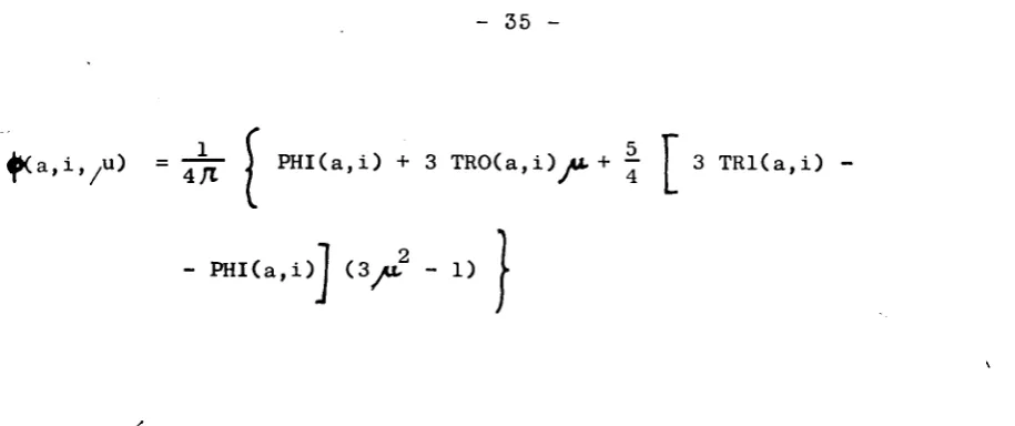
4><a,i,/0 = ^

Σ

(2L+i)g

(i)P

(

)

L

The first three polynomials are:

P

o =

'

l

=r

·

2

Ι

^ ­

(1)

and

1

y>o(i) = 2/f j d^L1/L2,i,jU.) = PHI(L1/L2^i) + PHI (1^/1^,1)

1

^ ( i ) = 2 ^ U i ^ a ^ L g , !,_/*) ­ TRO(L1/L2,i) ­ TROiL^L^i)

o

Í .

,

^2( i ) = 7Γ J 3/t d/L<b(L1/L2,i,/t) ­ Jt I d^^(L1/L2,i,/t) «

= | TR1(L1/L2,i) + TR1(L2/L1) ­ | PHI(L /L fi) + ΡΗΙζΙ^Λ, ,i)

Inserted into eq. (1) one obtains if PHI (L /L ,i) + PH1(L /L ,i) is set to

X Ci Δ X

^Ka,ivu) = - ~ \ PHKa.i) + 3 TRO(a,i)yU­+ | 3 TRl(a,i) ­

­ PHI(a,i)J (3^u­2 ­ 1) !■

For the special case ju. - 1, i.e. the angular flux perpendicular to the sur­

face, the (= 4i/t equivalent flux) 4 p Φ (a, i, ju = 1) is printed in a bivariate

table for all energy groups.

For the purpose of control also the angular flux in a solid angle of 2 stera­

dion is sampled around the surface normal and printed as the 4 Jl ­equivalent

flux. It refers only to the transmission L to L and is listed in the table

­L Ci

under the subtitle:

4*PI E Q I . OF 2 STERA. AVA.

FL*DE(L / L ) = 2

P-X et

[ Σ Σ

Vg/ÍA,g|

+

h

g C / O

+

Ι Σ

w

\ r

η g(yu. )

g(ytt ): Summation over g only for yu· \0.682.

The values 4 ƒ* <p(a,i, >u = 1) obtained by the Ρ -approximation are listed

under the heading:

36

-FLxDEÍL^/L,^ = P H I ( a , i ) + 3*TR0(a,i) + | | 3 * T R l ( a , i ) - P H I ( a , i )

and

5.5 The ReRun Procedures

The Rerun procedure is either used to increase the number of histories

or to calculate a Small Effect in one or more geometrical regions after

the execution of the so-called "basic case".

5.5.1 The Rerun for_Increasing the Historv_Number

A calculation can be continued (for improving the statistics) if it has

reached completion or if the specified time TIMPMX on card 4 was

ex-ceeded. In both cases a Rerun File, containing all the necessary

infor-mation for continuation is stored on Data-set 10. The input for

con-tinuation consists of:

CARD COLUMNS FORMAT SYMBOL

1 1 - 6 0 15A4 C0MCA(N),N =1,15

C0MCA(N),N =1,15 has to agree with the title of the job

being continued

61 1A1 C0MCAQ7) = R(or RWS)

67 1A1 C0MCA(18) = R(or RERUN)

2 2 - 7 &RERUN

9 etc. NAMELIST NAMES as described below, &END

HMAX: see CARD 4 of the section 5.2.

HFMAX:

HPRINT:

38

-CARD COLUMNS FORMAT SYMBOL

HDPMX: see CARD 4 of the section 5.2,

HFDPZE :

HFDPMX:

NSPQSM:

QRERUN: "

5.5.2 The Rerun for Performing_a Small_Effect Calculation

The SMEC option allows the calculation of small effects in certain geometr

regions specified by LQS(N), N=l, LQSM (card 4 ) . If in the course of the r;

dom walk process a neutron enters such a specified region, its coordinates

all other characteristic parameters (energy, weight, direction, etc.) are

stored on Data Set 11 and the history is terminated. The results of this f

sampling procedure represent the "Basic Case". Its physical meaning would 1

the regions LQS(N) are black.

In a subsequent small effect calculation (RWS-SMEC-step), histories whose

parameters are stored on Data Set 11 are read consecutively from it - if

required splitted - and in the case of an eigenvalue calculation, ITER opt

iterated. Finally they are combined with the "Basic Case" stored on the Re:

file on Data Set 10.

There are two possibilities for Small Effect calculations:

A) A SMEC calculation which is performed for the isotope composition definí

CARD COLUMNS FORMAT SYMBOL

1 1 - 6 0 15A4 C0MCA(N),N=1,15

C0MCA(N),N=1,15 job identification corresponding to the basic case

61 1A1 C0MCA(16) = R (or RWS)

67 1A1 C0MCA(17) = S (or SMEC)

2 2 - 7 &RERUN

NAMELIST NAMES (See previous section)

&END

B) Small Effect Calculations which are performed for other isotope

positions of LQS(N), N = 1, LQSM than used in A ) . In this case the

com-plete input of NDP and RWS has to be repeated with the required changes

of the isotope mixtures of LQS(N) and the following changes of C0MCA(17)

of the job identification card.

Input Parameters for the 1st Link Job (NDP)

1 1 - 6 0 15A4 C0MCA(N),N=1,15

COMCA(N), N = 1,15 job identification corresponding to the basic case

61 1A1 C0MCA(16) = N

67 1A1 C0MCA(17) = N

2 as in the basic case with the exception of the changes necessary to '

20 to redefine the regions LQS(N), N = 1, LQSM.

Input Parameters for the 2nd L m k Job (RWS)

1 1 - 6 0 15A4 C0MCA(N),N-1,15

40

-CARD

2

to

4

COLUMNS

61 67

as in the

FORMAT

1A1 1A1

basic case.

SYMBOL

COMCA(16) COMCA(17)

6. PLOTGEOM: A PROGRAM FOR DISPLAY OF GEOMETRY BY MEANS OF A CALCOMP PLOTTER

6.1 Introduction

PLOTGEOM is a program for checking both the geometry subprogram and the

geometry input data of Monte Carlo particle transport codes. It applies

the geometry subprogram in a similar way to a random walk program. From

the points of intersection between the geometrical structure and a mesh

of lines of flight, PLOTGEOM generates a picture, representing a

cross-section of the geometry.

The version described here has been connected with the 05R-Geometry

Pro-gram (1).

The plot routines are completely described in (2). Other geometry and

plot programs can easily be incorporated.

6.2 Method

The user specifies a two-dimensional cross-section of the geometry by

giving its orientation with respect to the geometry coordinate axes and

the desired coordinates of the corners of the picture

The program generates a horizontal grid of lines (parallel to the x-axis

of the picture). covering the area of the desired picture (Notation: L ).

The constant distance t between the lines L and L is 0.07 cm in the

picture. The points of intersection with the medium boundaries are

42

corded. Using for the start point the notation P. and for the crossing

1 , 0

points P. . one can write the distance between the s t a r t and crossing Ì..1

point P. . as

d. . = Ρ . - Ρ i j i j 1,0

After having scanned line L. the following can be concluded. If

1+1

d. . ­ d.Jn

ι J 1+1»k _^

CU

then the linepiece P. . P.,, . is called a segment. If more than one i j i+l,k

Ρ . , satisfies the quoted condition then only the nearest one to P.

i+l,k M J i j

is taken.

Now we define a body as being one segment or a string of segments, so

that the endpoint of one segment is the begin point of the next segment,

If a body with a last point P. . already exists,the segment P. . P,.. ,

i , J ' i , J . 1+1Λ

i s connected to t h i s body and the l a s t point of that body becomes P . , , , . i + l , k If there i s no body having P. . as l a s t point>the segment P. p + 1 . i £

i » J i » J i+i , k

the first one of a new body and the program looks for a "head" to be

connected to P. .. This "head" has to be in the neighbourhood of P.

i»J i j

between L. and L. , and is found by the subroutine HEADTL. The same

1 l­l

principle as that for finding the segments is applied by HEADTL. This

subroutine uses however a refined and variable grid.

Calling the lines *& and the points ρ the distance O between Ji>

m m,n m

' . The first Ö used is — € . The start point is determined by:

Ρ ­ P. .

m,o i,j

- iVTi.

The length of / is 2 <f .

m

If there is a body with a last point Ρ and if on examining L no

ifJ i+l

segment Ρ Ρ,α.·, ,, i s found, then this body should be given a "tail",

i,j i+l,κ

This tail is determined by the subroutine HEADTL in the same way as a

head, but now between L and L .

The "worms" (head, body, tail) thus created are stored on disk.

If the horizontal scanning has been finished the same procedure is re­

peated in the vertical direction (parallel to the y­axis of the picture).

Finally the worms are concatenated as far as possible: head to tail,

head to head, tail to tail. The strings of worms formed in this way are

plotted.

Remarks :

1. The grid distance of 0.07 cm is based on a picture dimension of at

most 70 cm, so that no more than 1001 parallel lines L. are possible.

2. A maximum of 30 crossing points are accepted in one line. If the cross

section has more, two pictures must be made.

3. A closed surface, where the equivalent dimensions in the picture are

44

-of less than 0.07 cm in the picture may cause the contours to run

into each other.

4. The quoted dimensions can easily be changed in the program.

6.3 Input of the Program PLOTGEOM

The data deck consists of cards with a control function, so-called

direc-tive cards, and cards with data. Each action (thus also the reading of

data cards) is preceded by a directive card. The first card expected by

the program is therefore a directive card. Having finished the execution

of a directive, the program expects a new directive till it has executed

the directive #ST(#P. The format of a directive card is 20A4. In column 1

must be placed the Sf sign. The actual directive takes the column 2 till

5 inclusive. The rest of the card is free for comment. Cards without &

are automatically ignored.

Directives + supplementary data

¿TITLE - The program expects as next card a title card in the format 20A4.

¿DATA - The program expects the data cards for the geometry description.

N.B. For the 05R-geometry the 1st card contains the in- and output data set reference number in the 216 format.

¿STOP - The program is terminated.

SfNOCAlcomp - CALC is set .FALSE. .

tfHISTory - HIST is set .TRUE. . The initial situation is HIST=.FALSE. If HIST=.TRUE. the coordinates in the startpoint of the flight and in the points of intersection of the flight path with the geometrical structure are printed.

tfNØHIstory - HIST is set .FALSE. .

SflDESPrint - DESP is set .TRUE. . The initial situation is DESP=.FALSE. If DESP=.TRUE. the scaled data to be plotted will also be

printed.

JfNäDEprint

SMEDIa

SNØMEdia

røRIHin

DESP is set .FALSE. .

MEDI is set .TRUE. . The initial situation is MEDI=.FALSE. If MEDI=.TRUE. the program expects in the following cards the coordinates of points in the geometry. For these points the medium numbers will be plotted in the picture. The pro-jection of such a point on the picture determines the lower left position of the plotted symbol(s). It is clear that this directive only has meaning if it follows SfPAUT. The expected cards are:

A: Format (I6.E12.5)

a - The number of points

b - The height of the numbers, to be written, in CM. a,b,c

B: Format (3E12.5) a - x-coordinate b -

y-c -

z-ti II

SfNØØRigin

For each point there has to be one card.

- MEDI is set .FALSE. .

- ØRIG is set .TRUE. . The initial situation is ORIG=.FALSE, If CfRIG=.TRUE. the program expects in the following card two numbers X and Y in the Format (2E12.5). These numbers are used in the plot of the scale numbers along the X-and Y-axis of the design as the origin.

46

-tfPLINe

SfPPNT

¿PAUTomatic

- The program expects in the next card the coordinates XI, Yl, ZI of point PI and the coordinates X2, Y2, Z2 of point P2. Format (6E12.5). Next, PI and P2 are connected and all points of intersection will be printed.

- The program expects in the next card the coordinates XI, Yl, Zl of point PI. Format (3E12.5). Next, the material in PI is printed.

- The program expects the following cards:

Card A: Format (6E10.5)

a. XO the coordinates of the point in the geo-b. YO metry that forms the lower left corner of c. ZO the picture.

d. XI The coordinates of the point in the geo-e. Yl metry that forms the upper right corner f. Zl of the picture.

Card B: Format (6E10.5)

a. XD These parameters are proportional to the b. YD direction cosines of the direction of the c. ZD Y-axis of the design.

d. XA These parameters are proportional to the e. YA direction of the direction of the X-axis f. ZA of the design.

Card C: Format (3E10.5)

a. XCM The width of the picture b. YCM The height of the picture

c. SCFGT The scale factor from real measures to picture. Remark: a,b or c should be in-dicated.

Next, the program starts the scanning of the defined plane in order to create the lines of intersection of plane and geometrical structure. If CALC has been set. TRUE, these pieces of the picture are temporarily stored on disk and afterwards loaded on the Calcomp tape.

Remarks :

may happen that, due to rounding errors, the last line of flight is outside the geometry. The 05R program will then stop. In such a case one should keep the picture a bit in the geometry.

2. The use of direct access input/output statements in subroutine PL0TG1 makes the definition of two data files on scratch disks necessary. The plot subroutines used in this version store the data to be plotted on data set 16.

The DD cards used at the Euratom installation are:

//Gd.FTOlFOOl DD DCB=(RECFM=F,LRECL=7200), // SPACE=(CYL,100),UNIT=SYSSQ, // DISP=(NEW,DELETE,DELETE), // V0L=SER=(EURSY2)

//GÍÍ.FT02F001 DD DCB=(RECFM=F,LRECL=72O0), / / SPACE=(CYL,100),UNIT=SYSSQ, / / DISP=(NEW,DELETE,DELETE), / / V0L=SER=(EURSY3)

//Gd.FT16F001 DD UNIT=TP9,LABEL=(,,,ÄJT),

// DSN=dsname, VÄUME=(PRIVATE, SER=EUnnnn ) , // DCB=(,DEN=2,TRTCH=C,RKCFM=VS, // LRECL=.484,BLKSIZE=488)

6.4 Short Description of the Program

The program deck to be used consists of four groups of subroutines.

1. The PLOTGEOM Programs:

Name Subroutines used

MAIN PLOTGM

PLOTGM PLINPT, PLOTG1, PLSCAN, PLOTG5, PLOTG4

- 48

PLOTDS PLSCAN HEADTL PLOTGl (PLOTG2) (PLOTG3) (PLOTG4) (PLOTG5) (PLOTG6) (PLFIN)

CRØSS

PLINE PLPNT AXPL HEAD (HEADR)

BLOCK DATA

PLOTG2, CROSS, HEADTL, PLOTG3 CROSS

FINIM, SYMBL4, AXPL, HEAD, LINE, PLMED, NUMBER, FINTRA

START, PATH CRØSS

PLMED

NUMBER, PLØT

2. The connecting programs between the PLOTGEOM and the Geometry Programs:

Name Subroutines used

PLMED INPUT START PATH

START JOMIN LOOKZ GEOM

3. The plot programs (see (2))(in Ispra in the System Library)

FINIM FINTRA LINE NUMBER SYMBL4 PLOT

6.4.1 Explanation regarding some important subroutines

The dimension of the vector X in COMMON (used in the 05R Geometry for data storing) is defined in the MAIN program. The MAIN program calls PLOTGM which executes the following steps:

1. Calls PLINPT which reads and prepares the input. 2. Calls PL0TG1 to prepare the plotting.

3. Prepares the parameters for the horizontal scanning.

4. Calls PLSCAN which scans the cross section in the horizontal direction of the picture. The "worms" are stored on disk.

5. Prepares the parameters for the vertical scanning. 6. The same as in 4., now in the vertical direction.

7. Calls PLOTG5 to concatenate the "worms" from disk and to plot the strings thus formed.

8. Calls PLOTG4 to position the coordinates for the next desigif. 9. Return to 1.

Subroutine PLINPT reads and interprets the directives. It reads, prints and stores the connected data. With the exception of PAUT all directives are executed by PLINPT calling the appropriate subroutines. In the case

of PAUT the control returns to the calling program PLØTGM.

Subroutine PLOTGl with the other entries PL0TG2, PL0TG3, PLOTG4, PL0TG5,

PL0TG6 and PLFIN takes care of the plotting. It stores, retrieves, scales and plots the desired data. All plot routines are called by means of this

­ 50

Subroutine PLMED (Χ,Υ,Ζ,M)

Determines in the point (Χ,Υ,Ζ) the material number M.

Subroutine INPUT

Calls for the input subroutines of the geometry program after having de­

termined the necessary arguments.

Subroutine START (ΧΒ,ΥΒ,ΖΒ)

Sets the parameters in the geometry program for a flight vector starting

in the point (ΧΒ,ΥΒ,ΖΒ).

Subroutine PATH

Computes the distance from the actual position along the line of flight

to the next point of intersection.

6.5 Description of COMMON and Variables

/PLGE1/ shared by PLØTGM. CRØSS

XC YC ZC

XPDEL

XREST

XE YE ZE

IX

The direction cosines of the line of flight.

The distance between two sequential points of intersection,

The remaining part of the line of flight.

The coordinates of the endpoint of the line of flight.

Event index = 0 = intersection.

/BLPATH/ Shared by CROSS. PATH

Start point of the line of flight. XP

YP ZP

/PLGE2/ Shared by PLSCAN. HEADTL. PLOTGM

XP1 YP1 ZP1

A

EPS

DXD DYD DZD

XA YA ZA

IENT

IMAX

XD YD ZD

The lower left point of the picture in the geometry (point PI)

The distance from PI to the lower right point.

The distance between two normal parallel lines of the grid.

The increments of the start coordinates for the next parallel line of the grid.

The direction cosines of the actual lines of the grid.

A counter for the number of CALL'S of CRØSS.

The number of grid lines.

The direction cosines of the normal of the grid.

/PLGSPE/ Shared by BLØCK DATA. CRØSS. PLINPT. PLOTGM

SPECIF(20) Images of specifications (directives).

SQ(20) Logical variables defining the state of the corresponding speci-fication in SPECIF.

/PLGE3/ Shared by PLSCAN. HEADTL. CRØSS

JC The number of intersections made in subroutine CRØSS.

- 52 /PLDATA/ LH(30) LT(30) PDX(1005,30) PDY(1005) NXK30) LXK30) HPDX(10,30) HPDY(10,30) TPDX(10,30) TPDY(10,30)

Shared by PLSCAN. PLØTG1

Nb. of head points

Nb. of tail points

x-coordinates of body points

II II II It

y-Index first point of body

11 - , Il II II

last

x-coordinates of the heads

II

y-II y-II y-II

X

-

y-Il II . ! . - , _

tails

Il II II

/PLGE4/

xo

YO ZO 3 XHR ;

YHR :

ZHR :

XWR YWR ZWR

Shared by PLOTGM. PLOTDS. PLOTGl

Geometry coordinates defining the lower left corner of the picture.

The direction cosines of the y-axis of the picture.

The direction cosines of the x-axis of the picture.

WRECTA HRECTA XCM YCM SCFCT DELD

The dimension of the cross section along the x-axis.

The dimension of the cross section along the y-axis.

The width of the picture = WRECTAxSCFCT (CM).

The height of the picture = HRECTAxSCFCT (CM).

The scaling factor.

SCANX Logical constant. True = Scanning in horizontal mode. False = Scanning in vertical mode.

/PLGE5/

NBMED

SYMBH

C0MED(3)

XØR YØR

Shared by PLINPT. PL0TG1

The number of points of the geometry of which the medium number should be plotted.

The height of the number to be plotted in CM.

The coordinates of the points.

Values of the graduation in the origin of the design.

6.6 References

(1) D.C. Irving, R.M. Freestone,Jr., F.B.K. Kam - 05R, A General Pur-pose Monte Carlo Neutron Transport Code, Oak Ridge 1965, ORNL-3622.

(2) P. Moinil, J. Pire - Programmation Relative au CALCOMP, Ispra 1965, EUR 2280.f.

6.7 Sample Problem

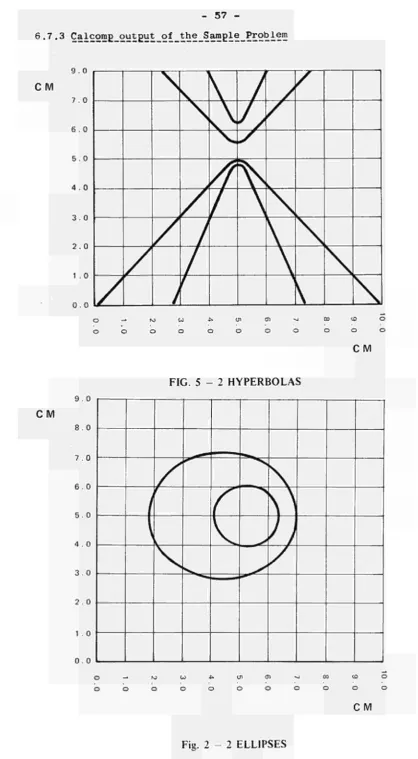
6.7.1 Input Data for the Sample Problem

Σ

5 6

2 MALE

X-ZQNE BCUftÉ - 5 . O O G Y-ZONE BOAJN - 5 . 0 0 C Z-ZQNE ÖCUN - 5 . 0 0 G

ZUNE 1 1

BLOCK ÜOONX - 5 . 0 0 Ô BLOCK Ö04JNY - 5 . 0 0 Ö BLOCK βΟΙΙΝΖ - 5 . 0 0 0

BLOCK 1 1

MEDIA 1»

SURFACES 1 ,

SECTOR - 1 SECTOR 1 SECTUR

2

1.0

-$PAUT 5 . 0 - i . O

5 . 0 0 0 5 . 0 0 0 5 . 0 0 0

5.COO

5.000

5.000

0

­1

0 1

CUADRA!IC

XSJ

XSJ

2,

2

SLRMCES

U

YSQ

ÍCUNLS1

YSU

A

Β

C

0

E

F

G

H

J

K

L

IM

2M

3M

­0.25

­ 1 .

ZSG

_ZSQ

¿ ELLIPSES

­5.C

O.C

STIILE

FIG.5 ­ ¿ HYPbRBÚLAS

SPAUT

6 . 7 . 2 Output of Sample Problem

S DATA

2 MALE

X - Z D N E BOUN - 0 . 5G000D 01» Y-ZDNE BOUN - 0 . 500OOD 0 1 , Z-ZDNE BOUN - C. 500CCD 0 1 ,

ZONE 1 1 1

BLOCK BÜUNX - 0 . 5 0 0 0 0 D 0 1 , BLOCK BOUNY - 0 . 5 0 0 0 0 D 0 1 , BLOCK BOUNZ - 0 . 5 0 0 0 O D 0 1 ,

O. 5 0 0 0 0 D 0 1 0 . 5 0 0 0 0 D 0 1 0 . 5 0 0 0 0 D 0 1

0.50000D 01

0.50000D 01

0.50000D 01

BLOCK 1

MEDIA SURFACES

SECTOR - 1 0

SECTOR 1 - I

SECTOR 0 1

2 QUADRATIC

0 . 1 0 0 0 OD 01XSQ 0 . 10C0 0D 01XSQ

1 ,

1 , 2 , 2

SURFACES ICONES)

0 . 1 0 0 0 0 D D1YSQ

0 . 1ÜO00D 0 1 YSQ - 0 . 2 5 0 Ü O D OOZSQ - 0 . 1 Û 0 G Û D 01ZSQ $ *

iCALCOMP

Í T I T L E

P L 0 T G E 0 M * * F I G . 2 - 2 E L L I P S E S

$PAUT

PARAMETERS USED

X 0 = Y 0 = · Z 0 =

-X l = · Y l » Z l =

XD=

-YD» Z D =

XA = YA = ZA = XCM = YCM=

SC FC Τ

0 . 500 OOE ■ 0 . 5 0 0 C O E •C.40COOE

- 0 . 50C00E 0 . 500COE 0 . 0

- 0 . l O O C O E 0 . 0

0 . 0

0 . 0

C . 9 2 8 4 8 E 0 . 3 7 1 3 9 E

m

0 . 1 0 7 7 0 E 02 0 . 1 0 0 0 0 E 0 2

0.10COOE C I

SUBROUTINE CROSS HAS BEEN ENTERED 2 3 3 T I M E S

SUBROUTINE CROSS HAS BEEN ENTERED 4 1 3 T I M E S