Keynes’s missing axioms

Munich Personal RePEc Archive

Keynes’s missing axioms

Kakarot-Handtke, Egmont

University of Stuttgart, Institute of Economics and Law

14 May 2011

Online at

https://mpra.ub.uni-muenchen.de/43856/

Keynes’s Missing Axioms

Egmont Kakarot-Handtke*

Abstract

Between Keynes’s verbalized theory and its formal basis persists a lacuna. The conceptual groundwork is too small and not general. The quest for a comprehensive formal basis is guided by the question: what is the minimum set of foundational propositions for a consistent reconstruction of the money economy? We start with three structural axioms. The claim of generality entails that it should be possible to prove that Keynes’s formalism is a subset of the structural axiom set. The axioms are applied to a central part of the

General Theoryin order to achieve consistency and generality.

JELB41, E12, E24, E25, E31, E40

Keywordsnew framework of concepts; structure-centric; axiom set; full employment; emergent money; singularity; system immanent risk; profit; distributed profit; saving; investment; Allais-Identity

*_{Affiliation: University of Stuttgart, Institute of Economics and Law, Keplerstrasse 17, D-70174}

The Keynesian Revolution was intended as both, a radical change of economic policy and a groundbreaking paradigm shift. Keynes left no doubt about the scientific scope of theGeneral Theory:

The classical theorists resemble Euclidean geometers in a non-Euclidean world . . . . Yet, in truth, there is no remedy except to throw over the axiom of parallels and to work out a non-Euclidean geometry. Something similar is required to-day in economics. (Keynes, 1973, p. 16)

While the political impact of Keynes’s ideas surpassed that of his precursors by several magnitudes, the policy proposals themselves had already been popular in the economic literature of the 1930s (Laidler, 1999, p. 10). The ratification of Keynes’s scientific claims therefore depends on the question whether he was successful in formulating some kind of non-Euclidean economic theory. By invoking Euclid, Keynes committed himself to the methodological consensus since Adam Smith (Hollander, 1977) and Senior:

It [the axiomatic method] was introduced to economics inA.D.1836 by

Nassau William Senior in hisOutline of the Science of Political Econ-omyand is today more or less consciously adopted by most economic theorists as the way of theorizing in economics. (Stigum, 1991, p. 4)

Euclid’s path runs through the classical school (Halévy, 1960, p. 494) the neoclassi-cal school (Jevons, 1911, p. 21), to reach a new level of Walrasian abstraction in the 1960s (Debreu, 1959, p. x). The salient point of axiomatization is also recognized by some Post Keynesians:

. . . , before accepting the conclusions of any economist’s model as applicable to the real world, the careful student should always examine and be prepared to criticize the applicability of the fundamental pos-tulates of the model; for, in the absence of any mistake in logic, the axioms of the model determine its conclusions. (Davidson, 2002, p. 41), see also (1996, p. 49), (1998, p. 68), (2005, p. 402)

Euclid’s spark, though, does not seem to have ignited Keynesianism. But one cannotnotaxiomatize. J. S. Mill clearly enunciated the question that stands at the beginning of any and every scientific inquiry:

What are the propositions which may reasonably be received without proof? That there must be some such propositions all are agreed, since there cannot be an infinite series of proof, a chain suspended from nothing. But to determine what these propositions are, is theopus

magnumof the more recondite mental philosophy. (Mill, 2006, p. 746),

original emphasis

For if orthodox economics is at fault, the error is to be found not in the superstructure, which has been erected with great care for logical consistency, but in a lack of clearness and of generality in the premises. (Keynes, 1973, p. xxi)

Hence the question arises: why did Keynes not heed his own appeal and in earnest worked out the required non-Euclidean formal basis? Not the least advantage of axiomatization is that it serves efficiency and in Keynes’s case it would have precluded the question ‘what Keynes really meant’. There can be no conclusive answer because ‘Keynes, too, sometimes gave the impression of not having fully grasped the logic of his own system’ (Laidler, 1999, p. 281).

Keynes’s conceptual groundwork consists in the main of two equations (Y=C+I

andS=Y–C, ergoI=S,Keynes, 1973, p. 63). That formal basis is too small and

contains quite a number of tacit assumptions. The conjunction between the income and saving equation to, for example, wage rate, price, output, profit, or money is formally opaque (Heilbroner and Milberg, 1995, p. 52). That is the specific thesis with regard to Keynes’s approach.

The general thesis says that human behavior does not yield to the axiomatic method (cf. Hudík, 2011; Rosenberg, 1980), yet the axiomatization of the money economy’s fundamental structure is feasible. By choosing objective structural relationships as axioms behavioral hypotheses are not ruled out. On the contrary, the structural axiom set is open toanybehavioral assumption and not restricted to the optimization calculus (for details see 2011b).

The objective is to establish a formalism of maximum structural simplicity. We start with an axiom set that is free of behavioral specifications and subsequently approach the complexity of the real world by a process of consistent differentiation. The claim of generality entails that it should be possible to prove that Keynes’s basic formalism is a subset of the structural axiom set.

1 Axioms

The first three axioms relate to income, production, and expenditures in a period of arbitrary length. For the remainder of this inquiry the period length is conveniently assumed to be the calendar year. Simplicity demands that we have at first one world economy, one firm, and one product. Quantitative and qualitative differentiation is obviously the next logical step after having worked out the implications of the following three axioms (for details see 2011d, pp. 5-7).

Total income of the household sectorY in periodtis the sum of wage income, i.e. the product of wage rateW and working hoursL, and distributed profit, i.e. the product of dividendDand the number of sharesN.

Y =W L+DN |t (1)

Output of the business sectorOis the product of productivityRand working hours.

O=RL |t (2)

Consumption expendituresCof the household sector is the product of priceP and quantity boughtX.

C=PX |t (3)

A set of axioms cannot be assessedex ante, because the full range of implications is not immediately transparent (Klant, 1984, p. 10). Self-evidence is neither necessary nor sufficient (Popper, 1980, pp. 71-72). Therefore, a set of axioms is either agreed upon as atentativeformal starting point or prematurely rejected out of hand. The assessment of axioms comes at the second stage with the interpretation of the logical implications of the formal world and the comparison with selected data and phenomena of the real world.

Axioms should have an intuitive economic interpretation (von Neumann and Morgenstern, 2007, p. 25), (Chick, 1998, pp. 1860-1861). The economic meaning is rather obvious for the set of structural axioms. What deserves mention is that total income in (1) is the sum of wage income anddistributed profitand not of wage income and profit. Profit and distributed profit have to be thoroughly kept apart. All structural axiomatic variables are measurable in principle.

2 Definitions

Definitions are supplemented by connecting variables on the right-hand side of the identity sign that have already been introduced by the axioms (Boylan and O’Gorman, 2007, p. 431). With (4) wage incomeYW and distributed profit income

YDis defined:

With (5) the expenditure ratioρE, the sales ratioρX, the distributed profit ratio

ρD, and the factor cost ratioρF is defined:

ρE ≡C

Y ρX ≡

X

O ρD≡

YD

YW ρF ≡

W

PR |t. (5)

Definitions add no new content to the set of axioms but determine the logical context of concepts. New variables are introduced with new axioms.

3 Nothing simpler than that

The axioms and definitions are consolidated to one single equation:

ρFρE(1+ρD)

ρX =1 |t. (6)

Theperiod core(6) as the absolute formal minimum determines the

interde-pendencies of the measurablekey ratiosfor each period. The period core is purely structural, i.e. free of any behavioral assumptions, unit-free because all real and nominal dimensions cancel out,1 and contingent. Contingency means that it is open until explicitly stated which of the variables are independent and which is dependent. The form of (6) precludes any notion of causality; it simply states the

interdependenceof the key ratios. The period core represents the pure consumption

economy, that is, no investment expenditures, no foreign trade, and no taxes or any other state activity.

The factor cost ratioρF summarizes the internal conditions of the firm. A value

ofρF <1 signifies that the real wage is lower than the productivity or, in other words, that unit wage costs are lower than the price, or in still other words, that the value of output exceeds the value of input. In this case the profit per unit is positive. Then we have the conditions in the product market. An expenditure ratioρE=1

indicates that consumption expenditures are equal to income and a value ofρX =1

of the sales ratio means that the quantities produced and sold are equal in periodtor, in other words, that the product market is cleared. In the special caseρE =1and

ρX =1 with market clearingandbudget balancing the profit per unit is determined

solely by the distributed profit ratioρD>0. In one sentence: the period core covers

the key ratios about the firm, the market, and the income distribution and determines their mutual interdependencies.

1 _{“This procedure is in accordance with the principle of objectivity requiring that the whole theory}

and its interpretations have to be independent of the choice of the units of measurement. And this requirement is met, if the theory is unit-free, the necessary condition stated in Buckingham’s

4 Employment

The first markedly Keynesian relation that follows from the period core (6) is the structural employment equation:

L= YD

PRρX

ρE−W

|t. (7)

As a purely formal relationship the period core must hold ineachperiod. Its new form now implies theadditionalassumption that employment as dependent variable is determined by the rest of the system. This is an assumption about the direction of dependency in a system with complex and mutual interrelations and this

add-onassumption is not implied in the axiom set which is clearly open to various

dependency interpretations. Dependency is conceptually different from causality. The structural employment equation states – with the other variables unaltered in each case:

(i) An increase of the wage rate leads tohigheremployment, i.e. to a lower unemployment rate.

(ii) A price increase is conductive toloweremployment.

(iii) Provided that wage rate, price and distributed profit all change with the same rate (W...=...P=Y...Dsee Section 6) there is no effect on

employ-ment.

(iv) If the configuration of price and wage rate changes is such that the denominator remains unchanged then employment stays where it is, no matter how large wage rate and price changes are. In this case perfect wage-price flexibility has no impact on employment (cf. Hahn and Solow, 1997, p. 134).

(v) An increase of the expenditure ratioρE leads to higher employment.

An expenditure ratioρE >1 presupposes the existence of a banking

system (see Section 7).

(vi) A productivity increase leads to lower employment.

(vii) As the difference in the denominator approaches zero employment goes (formally) off to infinity. This singularity is an implicit property of the economy as given by the structural axiom set (see Section 10).

(viii) Distributed profits exert a positive influence on employment.

capture reality the logical implications are observable. Equation (7) contains the originalPhillips curve as special case.2

With regard to the process of adaptation of employment to changes of the independent variables (7) implies that the independent variables have to be fixed at the beginning of the period under consideration. Since the period length is arbitrary no great distortions arise from this idealization if the length is conveniently chosen.

5 Full employment conditions

The standard key variable for the establishment of full employment is the real wage

W

P which has to fall (Keynes, 1973, p. 17). The structural axiomatic approach asserts

that in the consumption economy employment is determined by the expenditure ratioρE and the factor cost ratioρF =_PRW of which the real wage is a constituent.

This follows from (7) under the conditions that the product market is cleared, i.e.

ρX =1, and that the relation of dividend to wage rateρV is held constant:

L=

DN PR

ρX

ρE−

W PR

= ρVN

ρX

ρEρF−1

= ρVN

1

ρEρF−1

if ρX =1; ρV ≡ D

W |t.

(8)

Employment depends in the pure consumption economy on the relation of consumption expenditures to incomeρE, i.e. on the axiomatic version of Keynes’

effective demand (Keynes, 1973, pp. 23-24),3 (Kaldor, 1988, p. 153) and the outcome of the market price mechanism, i.e. the relation of wage rate, price, and productivityρF.

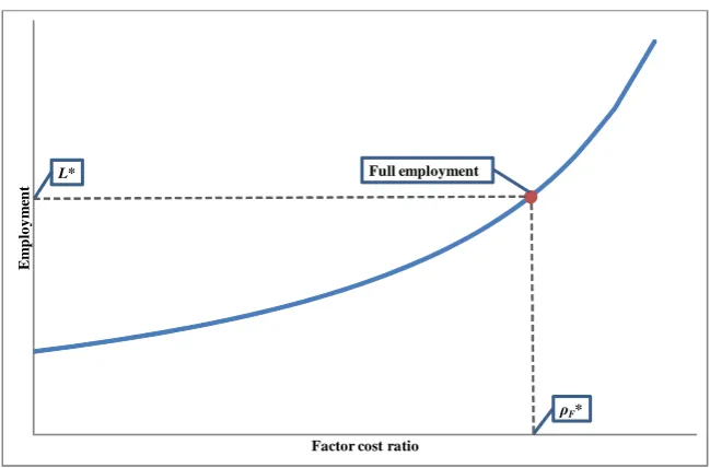
Under the conditions that the product market is cleared, i.e. ρX =1,and the

household sector’s budget is balanced, i.e. ρE =1, a higher factor cost ratio ρF

means higher employment as shown in Figure 1. The curve entails that there is no such thing as a natural rate of unemployment.4

There exists a unique factor cost ratioρ_F⋆, and by consequence a unique real

wage, that is consistent with full employment (however defined). From (8) follows as desideratum that condition (9) is satisfied:

2 _{It is noteworthy that Phillips “had not made an explicit link between inflation and unemployment”}

(Ormerod, 1994, p. 120). It was the Samuelson–Solow version of the ‘Phillips’ curve that ultimately failed, and (7) explains why.

3 _{The explicit inclusion of the consumption function determines the expenditure ratio as follows:}

ρE=_Ya+b.

E

m

p

lo

y

m

en

t

Factor cost ratio

ρF*

Full employment

L*

Figure 1:Structural relationship between factor cost ratio and employment(ρE=1)

ρ_F∗= 1 ρVN

L⋆ +1

or

_W

P

⋆

= R

ρVN

L⋆ +1

if ρX =1;ρE =1 |t. (9)

The numerical value ofL⋆_{depends on the actual definition of full employment.} If (9) is satisfied the product and the labor market is cleared and the budget is balanced. Since this result follows without regress to behavioral assumptions directly from the axioms it would be conceptually inappropriate to refer to this configuration as full employment equilibrium. Equilibrium would in addition require some economic mechanism which guarantees thatρF speedily approaches

ρ_F⋆. No such mechanism is known.

The point to emphasize is: since the structure that is given by the axiom set does not adapt to behavior, behavior has to adapt to structure. For the economy as a whole the behavioral real-wage/marginal-productivity condition is inapplicable and has to give way to (9).

In the general case, the expenditure ratioρE is different from unity and the

condition for full employment reads:

ρFρE= 1

ρVN

L⋆ +1

Full employment, then, can be realized withany combinationof the expenditure ratio and the factor cost ratio that satisfies (10)5which in turn entails both, Keynes’s principle of effective demand and the outcome of the market price mechanism.

In order to establish full employment, business has to accept a lower profit ratio

ρQ. This ratio is inverse to the factor cost ratioρF and follows from (24) as:

ρQ≡ ∆Qf i

W L ⇒ ρQ≡

1

ρF −1 if ρX =1 |t. (11)

It can be said, then, that full employment is not prevented by a ‘high’ wage rate W or a ‘high’ real wageW_P but by a ‘high’ profit ratioρQ. It is the profit ratio that

has to fall as long as there is unemployment in the pure consumption economy. An increase of the wage rate lowers the profit ratio and thus necessitates an employment expansion to realize the sameabsoluteamount of profit. The general relationship between total profit and the factor cost ratio follows from (24) in combination with the employment equation (7) and is given by:

∆Qf i≡ 1−ρF

1

ρE−ρF

YD if ρX=1 |t. (12)

If the expenditure ratioρEisunitythen the effects of a higher factor cost ratioρF

(lower profit ratioρQ) are always exactly compensated for by a higher employment

and the overall impact on total profit is nil if distributed profits remain constant. With regard to total profit business could in this case beindifferentbetween different employment levels. If therelation between dividend and wage rate ρV is kept

constant, as in (8), then both distributed profit and profit rise and fall with the wage rate, i.e.YD= (ρVN)W .A constantρV simply amplifies the wage rate effect of (7).

From the accustomed perspective6it seems to be counter-intuitive that a wage rate reduction, which lowers the real wage and raises the profit ratio, coincides with lower employment. This dissonance between standard behavioralassumptions and structuralfactexplains why the usual recipe for more employment does not succeed in getting the economy out of a slump (cf. Leijonhufvud, 1967, p. 402). The microeconomic optimization calculus and Marshall’s pair of demand–supply scissors simply do not apply to the economy as a whole. When behavioral and structural logic are at odds, behavioral logic is conductive to frustrated plans and expectations. Neoclassical prescriptions deteriorate a underemployment situation.

5 _If

ρX=1,ρF=1, andρE=1 thenρD=0,i.e.YD=0, according to (6). In this limiting case employment is indeterminate.

6 _{“It is a well-known generalisation of theoretical Economics that a wage which is held above}

the equilibrium level necessarily involves unemployment . . . . This is one of the most elementary deductions from the theory of economic equilibrium.” (Robbins, 1935, p. 146), for a commentary see (Weintraub, 1978).

6 The intermediate situation

The period values of the variables are connected formally by the familiar growth equation, which is added to the structural set as the 4th axiom:

Zt =Zt−1(1+

...

Z) Z|W,P,R,ρE (13)

The path of the representative variableZt, which stands here for wage rate, price,

productivity, and the expenditure ratio, is then determined by the initial valueZ0

and the rates of change...Zt for each period:

Zt=Z0(1+

... Z1) (1+

...

Z2). . .(1+

... Zt) =Z0

t

∏

(1+...Zt) (14)

Equation (14) describes the paths of the variables with therates of changeas unknowns. These unknowns are in need of determination and explanation. Since we do not wish to get involved into speculations about human behavior at this stage (for details see 2011g), we have to choose the random hypothesis because:

The simplest hypothesis is that variation is random until the contrary is shown, the onus of the proof resting on the advocate of the more complicated hypothesis . . . (Kreuzenkamp and McAleer, 1995, p. 12)

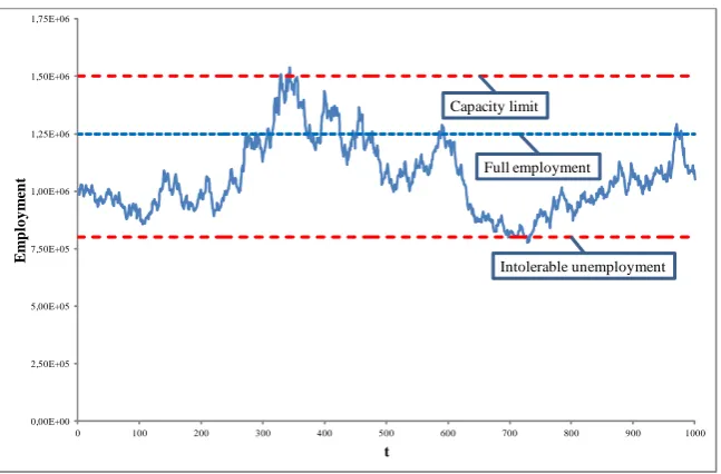
By feeding the employment equation with random rates of change for wage rate and price (1.000 changes between 0% and 0.4%) employment in this simple random economy develops over time as shown in Figure 2.7 Since all other variables are kept constant employment changes depend alone on changes of the real wage. Real wage and employment arepositivelyrelated (cf. Hahn and Solow, 1997, p. 136).

In the selected simulation employment remains within a corridor with the lower bound defined as intolerable unemployment and the upper bound defined as capacity limit. Full employment is somewhere in between. Keynes characterized the situation as follows:

In particular, it is an outstanding characteristic of the economic system in which we live that, whilst it is subject to severe fluctuations in respect of output and employment, it is not violently unstable. . . . Fluctuations may start briskly but seem to wear themselves out before they have proceeded to great extremes, and an intermediate situation which is neither desperate nor satisfactory is our normal lot. (Keynes, 1973, pp. 249-250)

In structural axiomatic terms our normal lot is explained by the probability that employment stays within the corridor. Yet this probability is not unity. There

7 _{The term random economy has been introduced for the equilibrium analysis of pure exchange}

0,00E+00 2,50E+05 5,00E+05 7,50E+05 1,00E+06 1,25E+06 1,50E+06 1,75E+06

0 100 200 300 400 500 600 700 800 900 1000

E

m

p

lo

y

m

en

t

t

Intolerable unemployment Full employment

Capacity limit

Figure 2:Keynes’s intermediate situation (with no singularities)

is a positive probability for a singularity, that is, employment mayformallygo off to infinity andactuallypress against the capacity limit for a longer time span. A situation that is prone to inflation (see Section 10). And there is a positive probability that employment falls below the tolerable level of unemployment (in whatever sense). The probability for the intermediate situation therefore depends on the width of the corridor and the fluctuations of the real wage, that is, on therelative magnitudes of the random rates of change of wage rate and price (Leijonhufvud, 2009, p. 750).

The invisible hand takes effect trough the law of large numbers and there is no such thing as a full employment equilibrium. There is no disequilibrium either. The intermediate situation becomes more complex, of course, when all independent variables of the employment equation vary at random. But this does not alter the fundamental structural fact that the probability for the intermediate situation is belowunity. This in turn implies that the economy cannotalwaysleft to itself.

7 Money

The money economy is thereal economy. The dichotomization of the real and the monetary sphere is the central point of Keynes’s methodological critique of orthodox economics:

Therefore, the first task is to show how money consistently follows from the given axiom set (for details see 2011e).

If income is higher than consumption expenditures the household sector’s stock of money increases. It decreases when the expenditure ratioρE is greater than unity.

The change of the household sector’s stock of money in periodtis defined as:

∆MH≡Y−C≡Y(1−ρE) |t. (15)

The stock of money at the end of an arbitrary number of periods is defined as the numerical integral of the previous changes of the stock plus the initial endowment:

MH≡

t

∑

∆MHt+MH0. (16)

The changes in the stock of money as seen from the business sector are symmet-rical to those of the household sector:

∆MB≡C−Y ≡Y(ρE−1) |t. (17)

The business sector’s stock of money at the end of an arbitrary number of periods is accordingly given by:

MB≡

t

∑

∆MBt+MB0. (18)

To simplify matters here it is supposed that all financial transactions are carried out without costs by the central bank. The stock of money then takes the form of current deposits or current overdrafts (Wicksell, 1936, p. 70). Initial endowments can be set to zero. Then, if the household sector owns current deposits according to (16) the current overdrafts of the business sector are of equal amount according to (18) and vice versa if the business sector owns current deposits. Money and credit are symmetrical; the stock of money of each sector can be either positive or negative. The current assets and liabilities of the central bank are equal by construction. From its perspective the quantity of money at the end of an arbitrary number of periods is given by the absolute value either from (16) or (18):

Mt ≡

t

∑

∆Mt

if M0=0. (19)

The quantity of money is always≥0. Equation (19) implies for a start that the central bank plays an accommodative role. Thus it is not necessary for the firms and households to resort to funds that have been accumulated before period1and we can

8 Endogenous and neutral

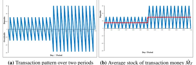
By sequencing the initially given period length of one year into months the idealized transaction pattern that is displayed in Figure 3 results (cf. Schmitt, 1996, p. 134). At the end of each subperiod the stock of money is zero. For the expenditure ratio in period1 ρE =1 holds. In period2 the wage rate, the dividend and the price is

doubled. Since no cash balances are carried forward from one period to the next, there resultsnoreal balance effect provided the doubling takes place exactly at the beginning of period2.

-30 -20 -10 0 10 20 30

0 60 120 180 240 300 360 420 480 540 600 660 720

O v er d ra ft s D ep o si ts

Day / Period

(a)Transaction pattern over two periods

-30 -20 -10 0 10 20 30

0 60 120 180 240 300 360 420 480 540 600 660 720

D

ep

o

si

ts

Day / Period

(b)Average stock of transaction money ˆMT

Figure 3:Graphical derivation of the average stock of transaction money from elementary transactions

From the perspective of the central bank it is a matter of indifference whether the household or the business sector owns current deposits. Therefore the pattern of Figure 3 translates into an average amount of current deposits. This average stock of transaction money depends on income according to the transaction equation

MT ≡κY |t (20)

which resembles Pigou’s Cambridge equation (the underlying theory is thereby not adopted).

For the transaction pattern that is here assumed as an idealization the index is ₄₈1. Different transaction patterns are characterized by different numerical values of the transaction pattern index.

Taking the definitions of the sales ratioρX and the expenditure ratioρE from

(5) one gets the explicit transaction equation:

(i) MT ≡κρX

ρE RLP (ii)

MT

P =κO if ρX =1;ρE =1 |t. (21)

ρE andρX are unity. Under theseinitialconditions money is endogenous (Desai,

1989, p. 150), (Nell, 1991, p. 187) and neutral (Patinkin, 1989a) in the structural axiomatic context. Money emerges fromautonomousmarket transactions and has three aspects: stock of money (MH,MB), quantity of money (hereM=0 at period

beginning and end; cf. Graziani, 1996, p. 143) and average stock of transaction money (hereMT>0). The quantity of money changes as soon asρE6=1, i.e. with

saving or dissaving. Then, the function of a store of value is activated.

9 Transaction money

The average stock of transaction money is given by (21). Taking the employment equation (7) into account, the definition of the average stock of transaction money boils down to what may be referred to as augmented transaction equation:

MT=κ ρVN

1

W−

ρE

PR

=(κ ρVN)W

1−ρEρF if ρX =1 |t. (22)

From this relation follows – with all other variables fixed in each case:

(i) An increase of the expenditure ratioρE leads according to (8) to higher

employment and exacts a higher average stock of transaction money MT according to (22).

(ii) When the rates of change of wage rate and price are identical employ-ment stays where it is andMT rises. Both, employment and the average

transaction balance remain unaltered if the rate of change of wage rate and price is zero.

(iii) A wage increase is conductive to higher employment and exacts a higherMT.

(iv) A price increase leads to a drop of employment and exacts a lower MT. Under the condition of budget balancing, i.e.ρE=1, and market

clearing, i.e.ρX =1, the varying configuration ofW, P, R,i.e. ofρF,

determines the development of the average stock of transaction money.

It is, in principle, possible to have a stable price, a rising stock of transaction money, wage increases marginally above productivity increases, and increasing employment. It is equally possible to have a stagflation if the price rises faster than the wage rate.

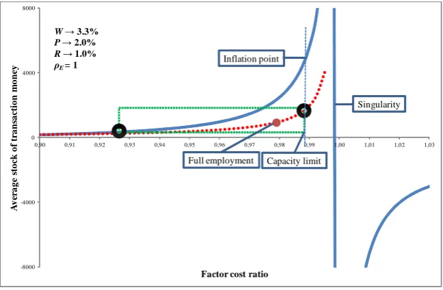
10 The singularity

stock of transaction money goes off to infinity. A glance at (22) reveals that this happens when the inverse of the expenditure ratio _ρ1

E is equal to the factor cost

ratioρF. Since both ratios vary independently this point moves unpredictably. The

singularity is the formal point of entry of system immanent risk and rather the opposite of equilibrium.

-8000 -4000 0 4000 8000

0,90 0,91 0,92 0,93 0,94 0,95 0,96 0,97 0,98 0,99 1,00 1,01 1,02 1,03

A v er a g e st o ck o f tr a n sa ct io n m o n ey

Factor cost ratio

W_{→ 3.3%} P→ 2.0% R→ 1.0%

ρE = 1

Singularity

Capacity limit Full employment

Inflation point

Figure 4:Structural singularity and goal compatible corridor

While the growth of the average stock of transaction money could go a long way, the coextensive employment expansion first reaches full employment and eventually runs against the capacity limit (if the factor cost ratio is increasedcontinuously, which of course does not occur in the random economy or in the real world). The augmented transaction equation cannot tell us more about what then happens. A new phenomenon must emerge. The circumstances suggest that the new phenomenon could be inflation.

11 Profit

The business sector’s financial profit in periodtis defined with (23) as the difference between the sales revenues – for the economy as a whole identical with consumption expendituresC– and costs – here identical with wage incomeYW:

∆Qf i≡C−YW |t. (23)

In explicit form, after the substitution of (3) and (4), this definition is identical with that of the theory of the firm:8

∆Qf i≡PX−W L |t. (24)

Using the first axiom (1) and the definitions (4) and (5) one gets:

∆Qf i≡C−Y+YD or ∆Qf i≡

ρE− 1

1+ρD

Y |t. (25)

In the pure consumption economy profit is greater than zero if the expenditure ratioρE is>1 or the distributed profit ratioρDis>0, or both. If distributed profit YDis set to zero, then profit or loss of the business sector is determined solely by the

expenditure ratio. For the business sector as a whole to make a profit consumption expendituresChave in the simplest case to be greater than wage incomeYW. So

that profit comes into existence in the pure consumption economy the household sector must run a deficit at least in one period. This in turn makes the inclusion of the financial sector mandatory. A theory that does not include at least one bank that supports the concomitant credit expansion, which is covered by (16), cannot capture the essential features of the market economy (Keynes, 1973, p. 85).9

It needs hardly emphasis that in the investment economy the process of profit generation appears more complex (for details see 2011f). This does not affect the nature of profit but simply removes theformalnecessity that thehouseholdshave to incur a deficit to get the economy going. This is then done by the investing business sector. It is not advisable, though, to tackle the complexities of the investment economy before the pure consumption economy is fullyunderstood. Mention should be made that neither neoclassicals nor Keynesians ever came to grips with profit (Desai, 2008, p. 10), (Tómasson and Bezemer, 2010).

12 A cognitive dissonance – but no contradiction

The determinants of profit look essentially different depending on the perspective. For the firm priceP, quantityX, wage rateW, and employmentLin (24) appear to

8 _{Nonfinancial profits are neglected here, i.e.}

ρX=1 throughout. For details see (2011a).

9 _{The purchase of all long lived consumption goods, e.g. houses, has to be subsumed under}

be all important; under the broader perspective of (25) these variables play no role at all. The profit definition provokes a cognitive dissonance between the micro and the macro view.

It is of utmost importance that profit∆Qf i and distributed profitYDis clearly

distinguished. The latter is a flow of income from the business to the household sector analogous to wage income. By contrast, profit is the difference of flows within the business sector (Keynes, 1973, p. 23). Profit is not connected to a factor input. So far, we have labor input as the sole factor of production and wage income as the corresponding factor remuneration. Since the factor capital is nonexistent in the pure consumption economy, profit cannot be assigned to it in functional terms. And since profit cannot be counted as factor income (cf. Knight, 2006, pp. 308-309, Schumpeter, 2008, p. 153), there is no place for it in the theory of income distribution. This would plainly be a category mistake (for details see 2012).

The individual firm is blind to the structural relationship given by (25). On the firm’s level profit is therefore subjectively interpreted as a reward for innovation or superior management skills or higher efficiency or toughness on wages or for risk taking or capitalizing on market imperfections or as the result of monopolistic practices. These factors play a role when it comes to thedistributionof profits between firms and these phenomena become visible when similar firms of an industry are compared. Business does not ‘make’ profit, it redistributes profit. The case is perfectly clear when there is only one firm. It is a matter of indifference whether the firm’s management thinks that it needs profit to cover risks or to finance growth or whether it realizes the profit maximum or not. If the expenditure ratio is unity and the distributed profit ratio is zero, profit will invariably be zero. The existence and magnitude of total profit is not explicable by the marginal principle. Because of this, it is not wise to take the considerations of the individual firm’s management as analytical starting-point and then to generalize. The microeconomic approach is inherently prone to the fallacy of composition. The profit definition entails a cognitive dissonance between micro and macro, but no logical contradiction. Ab originetotal profit is a factor-independent residual (Ellerman, 1986, pp. 61-65). This distinction is crucial.

We know from the history of science that entrenched classificatory schemes and misleading descriptive vocabularies have impeded scien-tific advance as much or more than the complexities and observational inaccessibility of the subject matter. (Rosenberg, 1980, p. 114)

Under the conditionρE =1 profit∆Qf i must, as a corollary of (25), be equal to

distributed profitYD. The fundamental difference between the two variables is not

an issue in thislimiting case. The equality of profit and distributed profit is an implicit feature of equilibrium models (Godley and Shaikh, 2002, p. 425), (Patinkin, 1989b, p. 329), (Buiter, 1980, pp. 3, 7). These havenocounterpart in reality.

because we have profit but no capital. And, since profit and capital must not be treated like Siamese Twins, as they have by the classics, the tendency of the profit rate to fall is also in need of a thorough revision (for details see 2011f, pp. 18-20). The question of whether in equilibrium profit is zero or not – Walras’s ‘ni bénéfice ni perte’ – is of no concern within the structural axiomatic framework because the notion of simultaneous equilibrium is noconstituent part of it (cf. Kaldor, 1985, p. 12). In the general case, profit or loss depends on consumer spending and profit distribution. If in the limiting case distributed profit in (25) is zero, then any loss of the business sector must be equal to the saving of the household sector as specified by (28). Since saving is – in the absence of distributed profits – the exact complement of loss, it must be overcompensated by dissaving within a short time interval, i.e.ρE >1, otherwise the economy faces major challenges. So the real question is not about the existence of a zero-profit equilibrium, but how the market economy can, and in fact does, avoid this predicament over a longer time span (Keynes, 1973, pp. 158-159), (Rotheim, 1981, p. 581).

The definition of profit (23) has another important implication. There is no real residual that corresponds to the nominal residual profit. Real (O, X) and nominal (Y, C) flows are to some degree independent. Profit belongsentirely to the nominal sphere, in a real model it cannot exist. This is the defining characteristic of what Keynes termed the entrepreneur economy (Rotheim, 1981, pp. 575, 577, 579).

13 Retained profit

Profits can either be distributed or retained. If nothing is distributed, then profit adds entirely to the financial wealth of the firm. Retained profit∆Qreis defined for the

business sector as a whole as the difference between profit and distributed profit in periodt:

∆Qre≡∆Qf i−YD |t. (26)

Using (25) and (17) it follows:

∆Qre≡nC−Y≡m∆MB |t. (27)

Retained profit∆Qre is the residualC−Y as it appears at the firm; the same

residual appears at the central bank as a change of the business sector’s stock of money∆MB. Thetwo aspectsare kept apart by the notation≡nand≡m, respectively.

14 Saving

Financial saving is given by (28) as the difference of income and consumption expenditures. This definition is identical with Keynes’s, i.e. ∆Sf i equates to the

KeynesianS. In combination with (15) this yields the straightforward relation:

∆Sf i≡Y−C ⇒ ∆Sf i≡nY−C≡m∆MH. (28)

Saving and the change of the household sector’s stock of money aretwo aspects of the same flow residual. It follows immediately that the development of the household sector’s stock of money is thus given by (16).

Financial saving (28) and retained profit (27) always move in opposite direc-tions, i.e.∆Qre≡ −∆Sf i. Let us call this the complementarity corollary because it

follows directly from the definitions themselves. The corollary asserts that the com-plementary notion to saving isnotinvestment but negative retained profit. Positive retained profit is the complementary of dissaving. Since there is no investment in the pure consumption economy the IS-equality-identity-equilibrium cannot hold. The complementarity corollary entails that the plans of households and firms are in the general casenotmutually compatible.

15 Allais is general

Having clarified the structural properties of the pure consumption economy we are now ready to assess the relation between the axiomatic and the Keynesian approach in still more detail. Based on the differentiated formalism it is assumed that the investment goods industry, which consists of one firm, producesOI=XIunits of an

investment good, which is bought by the consumption goods industry to be used for the production of consumption goods in future periods. The households buy but the output of the consumption goods industry (for details see 2011f). From (24) then follows for the financial profit of the consumption and investment goods industry, respectively:

∆Qf iC≡C−YWC ∆Qf iI≡I−YWI YW≡YWC+YWI |t. (29)

Total financial profit, defined as the sum of both industries, is then given by the sum of consumption expenditures and investment expenditures minus wage income which is here expressed as the difference of total income minus distributed profit:

∆Qf i≡C+I−(Y−YD) |t. (30)

From this and the definition of financial saving (28) follows:

∆Qf i≡I−∆Sf i+YD |t. (31)

distributed profits and lower saving on the other side and vice versa. By finally applying the definition of retained profit (26) the Allais-Identity follows:

∆Qre≡I−∆Sf i |t. (32)

Autrement dit l’investissement n’est pas égal à l’épargne spontanée, mais à l’épargne spontanée augmenté du revenue non distribué des entreprises . . . . (Allais, 1993, p. 69), see also (Robinson, 1956, p. 402), (Lavoie, 1992, p. 159 eq. (4.3)), (Godley and Lavoie, 2007, p. 37 fn 9)

If retained profit is zero, that is, if profit and distributed profit happen to be equal in (26), then, as a corollary, investment expenditures and household saving in (32) must be equal too. Vice versa, if it happens that household saving is equal to investment expenditure then, as a corollary, profit and distributed profit must be equal too. In reality, though, profit and distributed profit are virtuallyneverequal and correspondingly household saving and investment are not equal either. The fact that retained profit is different from zero in each period can be taken as an

empirical proof of the logically equivalent inequality of household saving and

business investment. Allais has definitively settled the IS-debate of the 1930s in 1993. Since then, all models – including IS-LM – that have been built and are still being built on the arguments of (Hicks, 1939, pp. 181-184), (Ohlin, 1937), (Lutz, 1938), (Lerner, 1938), (Keynes, 1973, p. 63), (Kalecki, 1987, p. 138) and others have to be regarded either as limiting cases or as formally deficient.

16 TreatiseandGeneral Theoryas limiting cases

When the profit definition for the pure consumption economy (i) in (33) and the investment economy (ii) is compared

(i) ∆Qf i≡YD−∆Sf i

(ii) ∆Qf i≡I+YD−∆Sf i (33)

the first point to emphasize is that definition (i) is consistently replaced by the broader definition (ii). The inclusion of the investment process significantly changes the scope of profit generation. This change, though, is opaque to the agents, which can perceive scarcely more than their firm’s sales revenues and factor costs. For definition (ii) the corollary (34) holds: if it happens that investment expenditures are zero then it must be the case that financial profit is equal to the difference of distributed profit and household saving, and vice versa. The corollary (34) replaces definition (i) in (33) and now applies to the pure consumption economy as a limiting case:

For definition (ii) a second corollary (35) holds: if it happens that distributed profit is zero then financial profit must be equal to the difference of investment expenditures and household sector’s saving:

YD=0⇔∆Qf i=I−∆Sf i |t. (35)

This implication of (ii) is well known as one of Keynes’s ‘fundamental equations for the value of money’ (Keynes, 1971, pp. 124, 136). This means that, although Keynes was closer to the axiomatic formalism in hisTreatisethan in hisGeneral

Theoryhe nonetheless was not general there either (cf. Hicks, 1939, p. 184). The

reason is that he, in accordance with orthodox economic theory, did not accurately discriminate between profit and distributed profit and by consequence failed to take into account the process of profit distribution that is crucial for the functioning of the market system. Structural axiomatization ultimately boils down to the rejection of Keynes’s definition:

Thus the factor cost and the entrepreneur’s profit make up, between them, what we shall define as thetotal income resulting from the employment given by the entrepreneur. (Keynes, 1973, p. 23), original emphasis

Total income consists in the simplest case of wage income anddistributed profits.

Toutes ses [Keynes’s] deductions, à notre avis, manquent absolument de rigeur. . . . L’intuition de Keynes lui a fait sentir où se trouvaient les difficultés, mais son insuffisance logique ne lui a pas permis de résoudre les problèmes que son intuition lui avait fait entrevoir. (Allais, 1993, p. 70)

17 Delicate distinctions

The present formalism is composed of axioms and definitions. In a strictly formal sense the definitions are dispensable. Any new symbol (definiendum) that is intro-duced with a definition is an abbreviation for a longer expression (definiens) that is composed of the variables of the axiom set and the familiar mathematical operators. So, when the word processor is instructed to replace one definiendum after another by its definiens then the equations become longer yet nothing else changes. No variables other than those of the axiom set remain.

Since it is true that everybody is free to define whatever appears to be appropriate it seems that a definition could not pose any real problem. This, indeed, isnottrue because the full freedom of definition holds but for the first definition. As Georgescu-Roegen put it:

most. (Georgescu-Roegen, 1970, p. 9), see also (Boland, 2003, p. 87), (Hahn, 1984, p. 40).

Let us suppose somebody looks at the Allais-Identity (32), which states that retained profit for the economy as a whole is equal to the difference of the business sector’s investment expenditure and the household sector’s financial saving, and proposes to refer to thesumof saving and retained profit astotal private savingΣbecause retained profit may, after all, well be regarded as saving of the business sector (e.g. Lavoie, 1992, p. 159). Thereby a new definition, (i) in (36), would be added to the already existing formalism. Together with the Allais-Identity (ii) this gives (iii) which states thattotal private savingΣ(andnothousehold saving∆Sf irespectively

Sin Keynes’s notation) “equals” investment:

(i) Σ≡∆Sf i+∆Qre (ii)∆Qre≡I−∆Sf i ⇒ (iii)Σ≡I |t. (36)

We thus arrive at an implicit definition that is no proper definition at all:

For a definition to be valid it must meet several conditions: (1) it must bedispensable, that is, the scientist must be able to do without it; and (2) it must benoncreative, that is, the scientist cannot use the definition to establish formulas that do not contain the defined term, unless these formulas can be proved without using the definition. (Stigum, 1991, pp. 35-36), original emphasis

Equation (36) (iii) is no dispensable abbreviation but simply permits the arbitrary

permutationof the symbolsΣandI. While the Allais-Identity contains valuable

information,Σ≡I≡Sis a homespun muddle. To defineΣand then to placeSfor

Σ_{is an elementary formal mistake.}

But, and this makes things a bit complicated, if it happens that retained profit is zero in (i) then, as a corollary, it must hold that total private savingΣand household saving∆Sf iareequal, i.e. Σ=Sf i. From (ii) then results as a corollaryI=∆Sf i

or in plain words: household sector’s saving equals investment –if retained profit is zero, whichneverhappens. In contrast, (iii) states that total private savingΣis identical with investmentI by definition (cf. Samuelson and Nordhaus, 1998, p. 204 and p. 194 for corporate saving10).

Acompleteresolution of this formally unacceptable state of affairs requires that the wrong turnoff (i) in (36) isnottaken. This definition implicitly leads to (iii) which signals redundancy. Redundancy calls for Occam’s razor.

Under the purely formal perspective the salient point is: in a system of equations x=ysignifies a condition that is satisfied by certain values of the unknowns; in a system of definitionsx≡ysignifies a dead end. The latter expression allows replacing the word apple wherever it appears by the word orange and vice versa. From this, no profound insights are to be expected.

10_{From the 1948 edition onwards, Samuelson never came to grips with profits (Tómasson and}

18 A look at the ledger

Under the conceptual perspective the salient point is: saving as the complement of consumption expenditures refersexclusivelyto the household sector.

It is true, of course, that neoclassical economists also considertotal private saving, defined as the sum of personal and business saving, since the distinction between households and firms is often treated as a veil and individual agents are assumed to optimize total private (rather than merely household) saving. (Gordon, 1995, p. 62), original emphasis

There isnosuch thing as saving of the business sector. Ultimately, the saving-equals-investment formula results in superficial empirical studies (Gordon, 1995, pp. 60-62) and unacceptable bookkeeping conventions in national accounting (cf. Eisner, 1995, p. 109; Godley and Lavoie, 2007, pp. 260-263). To demonstrate this, Figure 5 reconstructs the steps from pure transaction recording to the formally indefensible and ultimately futile collapsing of the business sector’s retained profit and the household sector’s saving (cf. Boulding, 1950, pp. 248-252, Levy and Levy, 1983, pp. 44-48).

Collapsing is futile because it just annihilates what has been gained by differ-entiation and because the result is predictable: all surpluses and deficits between economic units and all credit relations vanish. The very essence of economics evaporates.

Conceptual consistency prohibits the application of the notion of saving to the business sector. The compelling reason for rejecting the definition of total private savingΣin (36), andeverythingthat follows from it, boils down to that it is conceptually inadmissible, implicitly leads toΣ≡I, which signifies redundancy, and for certain conditions toI=∆Sf i, which is a limiting case of the Allais-Identity

withnoreal world correspondence.

19 Neverex ante, neverex post

Needless to emphasize that it did not got lost in the discussion that in fact investment expenditures might not be equal to household saving and this was explained with the perfect reconcilability of anex antedisequilibrium with theex postbookkeeping truismI≡S(Myrdal, 1939, p. 47), which in turn is different from the equilibrium conditionI=S. This rationalization is beside the point for the simple reason that a meticulous recording of all transactions during one period arrives at the Allais-Identity. Only after applying the indefensible definition of total private savingΣ

Figure 5:How the accountant produces valuable information before collapsing it away (CGI con-sumption goods industry, IGI investment goods industry)

not much for conceptual consistency. All that is necessary, then, is to add up the available numbers and to abstain from redundant definitions.

20 Set and subset

Axioms Definitions

(i) Y =W L+DN (iv) ∆Qf i≡PX−W L

(ii) O=RL (v) ∆Sf i≡Y−C

(iii) C=PX

(i⋆_{) Y =C+I}

if YD=∆Qf i

|t. (37)

The structural axiomatic approach rests on the three axioms (i)-(iii) that capture the elementary facts of a money economy and two definitions. It formally reduces to Keynes’s limiting case (i⋆_{) and (v) if profit is exactly equal to distributed profit} which, obviously, does not happen in the real world.

Keynes’s main concern in theGeneral Theorywas not market or policy failure but theory failure. By consequence he envisioned nothing less than a paradigm shift (Coddington, 1976) and called for a ‘complete theory of a monetary economy’ (Keynes, 1973, p. 293), see also (Dillard, 2010). While perfectly aware that this at the same time required a consistent set of some kind of non-Euclidean axioms, Keynes had no desire that the particular forms of his ‘comparatively simple fundamental ideas . . . should be crystallized at the present state of the debate’ (cited in Rotheim, 1981, p. 571). Hahn’s balanced view, though, might be closer to the mark:

I consider that Keynes had no real grasp of formal economic theorizing (and also disliked it), and that he consequently left many gaping holes in his theory. I none the less hold that his insights were several orders more profound and realistic than those of his recent critics. (Hahn, 1982, pp. x-xi)

From all this follows:

We are not time-locked by the particular (and provisional) choice Keynes made in expositing his ideas in 1936. (O’Donnell, 1997, p. 158)

21 Conclusions

Behavioral assumptions, rational or otherwise, are not solid enough to be eligible as first principles of theoretical economics. Hence all endeavors to lay the formal foundation on a new site and at a deeper level actually need no further vindication. The present paper suggests three non-behavioral axioms as groundwork for the formal reconstruction of the evolving money economy.

• The expenditure-income asymmetry is the indispensable prerequisite for

favorable business conditions and prolonged growth. This holds for the elementary consumption economy and the complex investment economy in equal measure.

• The key variables for the attainment of full employment are the expenditure

ratio, i.e. the axiomatic version of Keynes’ effective demand, and the factor cost ratio, i.e. the configuration of wage rate, price, and productivity as outcome of the market price mechanism.

• There is no structural trade-off between higher price inflation and lower

unemployment.

• The employment effect depends on therelativemagnitude of wage rate and

price changes.

• Higher employment is compatible with a higher real wage, a lower unit profit

ratio and unaltered profit for the business sector as a whole.

• Models that are based on the collapsed definition total income≡wages +

profits are erroneous because profit and distributed profit is not the same thing.

• The structural axiom set implies that it is possible to have a stable price, a

ris-ing stock of transaction money, wage increases marginally above productivity increases, and rising employment.

• There is no such thing as a natural rate of unemployment and it is not a ‘high’

nominal or real wage that prevents full employment but a ‘high’ profit ratio.

• The structural axiom set implies a singularity. A singularity is the point of

entry of systemic risk and rather the opposite of equilibrium.

• Keynes proposed to ‘throw over’ the axioms of the orthodox theorists which

‘resemble Euclidean geometers in a non-Euclidean world’, but failed to heed his own appeal. His own formal basis is too small, contains too many tacit assumptions, and is not general.

• The Keynesian formalism is a subset of the structural axiom set. The general

Allais-Identity is confirmed. With regard to allI=SorI≡Smodels it asserts that household saving is virtually never equal to investment expenditures, neitherex antenorex post. The standardex ante–ex postexplanation consists of multiple logical errors that support one another.

References

Allais, M. (1993). Les Fondements Comptable de la Macro-Économie. Paris: Presses Universitaires de France, 2nd edition.

Boland, L. A. (2003). The Foundations of Economic Method. A Popperian

Perspec-tive. London, New York, NY: Routledge, 2nd edition.

Boulding, K. (1950). A Reconstruction of Economics. New York, NY: Science Editions.

Boylan, T. A., and O’Gorman, P. F. (2007). Axiomatization and Formalism in Economics. Journal of Economic Surveys, 21(2): 426–446.

Buiter, W. H. (1980). Walras’ Law and All That: Budget Constraints and Balance Sheet Constraints in Period Models and Continuous Time Models. International

Economic Review, 21(1): 1–16. URLhttp://www.jstor.org/stable/2526236.

Chick, V. (1998). On Knowing One’s Place: The Role of Formalism in Eco-nomics. Economic Journal, 108(451): 1859–1869. URLhttp://www.jstor.org/ stable/2565849.

Coddington, A. (1976). Keynesian Economics: The Search for First Principles.

Journal of Economic Literature, 14(4): 1258–1273. URLhttp://www.jstor.org/

stable/2722548.

Davidson, P. (1996). Reality and Economic Theory. Journal of Post Keynesian

Economics, 18(4): 479–508. URLhttp://www.jstor.org/stable/4538504.

Davidson, P. (1998). Reviving Keynes’s Revolution. In D. L. Prychitko (Ed.),Why Economists Disagree, pages 68–82. Albany, NY: State University of New York Press.

Davidson, P. (2002).Financial Markets, Money and the Real World. Cheltenham, Northampton, MA: Edward Elgar.

Davidson, P. (2005). Responses to Lavoie, King, and Dow on What Post Keyne-sianism Is and Who Is a Post Keynesian.Journal of Post Keynesian Economics, 27(3): 393–408. URLhttp://www.jstor.org/stable/4538934.

Debreu, G. (1959).Theory of Value. An Axiomatic Analysis of Economic Equilib-rium. New Haven, London: Yale University Press.

Dennis, K. (1982). Economic Theory and the Problem of Translation (I). Journal

of Economic Issues, 16(3): 691–712. URLhttp://www.jstor.org/stable/4225211.

Desai, M. (2008). Profit and Profit Theory. In S. N. Durlauf, and L. E. Blume (Eds.),The New Palgrave Dictionary of Economics Online, pages 1–11. Palgrave Macmillan, 2nd edition. URLhttp://www.dictionaryofeconomics.com/article?id= pde2008_P000213.

Dillard, D. (2010). The Theory of a Monetary Economy. In K. K. Kurihara (Ed.), Post Keynesian Economics, pages 3–30. London, New York, NY: Routledge. (1955).

Eisner, R. (1995). US National Saving and Budget Deficits. In G. A. Epstein, and H. M. Gintis (Eds.),Macroeconomic Policy After the Conservative Era, pages 109–142. Cambridge: Cambridge University Press.

Ellerman, D. P. (1986). Property Appropriation and Economic Theory. In P. Mirowski (Ed.),The Reconstruction of Economic Theory, pages 41–92. Boston, MA, Dordrecht, Lancaster: Kluwer-Nijhoff.

Föllmer, H. (1974). Random Economies with Many Interacting Agents. Journal of Mathematical Economics, 1: 51–62.

Georgescu-Roegen, N. (1970). The Economics of Production. American Economic

Review, Papers and Proceedings, 60(2): 1–9. URLhttp://www.jstor.org/stable/

1815777.

Godley, W., and Lavoie, M. (2007). Monetary Economics. An Integrated Approach

to Credit, Money, Income and Wealth. Houndmills, Basingstoke, New York, NY:

Palgrave Macmillan.

Godley, W., and Shaikh, A. (2002). An Important Inconsistency at the Heart of the Macroeconomic Model. Journal of Post Keynesian Economics, 24(3): 423–441. URLhttp://www.jstor.org/stable/4538786.

Gordon, D. M. (1995). Putting the Horse (Back) Before the Cart: Disentangling the Macro Relationship Between Investment and Saving. In G. A. Epstein, and H. M. Gintis (Eds.),Marcoeconomic Policy After the Conservative Era, pages 57–108. Cambridge: Cambridge University Press.

Graziani, A. (1996). Money as Purchasing Power and Money as a Stock of Wealth in Keynesian Economic Thought. In G. Deleplace, and E. J. Nell (Eds.),Money in Motion, pages 139–154. Houndmills, Basingstoke, London: Macmillan.

Hahn, F. H. (1980). General Equilibrium Theory. Public Interest. Special Issue: The Crisis in Economic Theory, pages 123–138.

Hahn, F. H. (1982). Money and Inflation. Oxford: Blackwell.

Hahn, F. H., and Solow, R. M. (1997).A Critical Essay on Modern Macroeconomic Theory. Cambridge, MA, London: MIT Press.

Hall, R. E. (2011). The Long Slump.American Economic Review, 101(2): 431–469. URLhttp://www.aeaweb.org/articles.php?doi=10.1257/aer.101.2.431.

Halévy, E. (1960). The Growth of Philosophic Radicalism. Boston, MA: Beacon Press.

Heilbroner, R., and Milberg, W. (1995). The Crisis of Vision of Modern Economic Thought. Cambridge, New York, NY, Melbourne: Cambridge University Press.

Heilbroner, R. L. (1942). Saving and Investments: Dynamic Aspects. American

Economic Review, 32(4): 827–828. URLhttp://www.jstor.org/stable/1816763.

Hicks, J. R. (1939).Value and Capital. Oxford: Clarendon Press, 2nd edition.

Hollander, S. (1977). Adam Smith and the Self-Interest Axiom. Journal of Law

and Economics, 20(1): 133–152. URLhttp://www.jstor.org/stable/725090.

Hudík, M. (2011). Why Economics is Not a Science of Behaviour. Journal of Economic Methodology, 18(2): 147–162.

Jevons, W. S. (1911). The Theory of Political Economy. London, Bombay, etc.: Macmillan, 4th edition.

Kakarot-Handtke, E. (2011a). Primary and Secondary Markets. SSRN Working

Paper Series, 1917012: 1–25. URLhttp://ssrn.com/abstract=1917012.

Kakarot-Handtke, E. (2011b). The Propensity Function as General Formalization of Economic Man/Woman. SSRN Working Paper Series, 1942202: 1–28. URL http://ssrn.com/abstract=1942202.

Kakarot-Handtke, E. (2011c). Properties of an Economy Without Human Beings.

SSRN Working Paper Series, 1863788: 1–23. URL http://ssrn.com/abstract=

1863788.

Kakarot-Handtke, E. (2011d). The Pure Logic of Value, Profit, Interest. SSRN

Working Paper Series, 1838203: 1–25. URLhttp://ssrn.com/abstract=1838203.

Kakarot-Handtke, E. (2011e). Reconstructing the Quantity Theory (I). SSRN

Working Paper Series, 1895268: 1–26. URLhttp://ssrn.com/abstract=1895268.

Kakarot-Handtke, E. (2011f). Squaring the Investment Cycle. SSRN Working Paper

Series, 1911796: 1–25. URLhttp://ssrn.com/abstract=1911796.

Kakarot-Handtke, E. (2011g). Unemployment Out of Nowhere. SSRN Working

Kakarot-Handtke, E. (2012). Income Distribution, Profit, and Real Shares. SSRN

Working Paper Series, 2012793: 1–13. URLhttp://ssrn.com/abstract=2012793.

Kaldor, N. (1985).Economics Without Equilibrium. Armonk, NY: M.E. Sharpe.

Kaldor, N. (1988). The Role of Effective Demand in the Short Run and the Long Run. In A. Barrère (Ed.),The Foundations of Keynesian Analysis, pages 153–160. Houndmills, London: Macmillan.

Kalecki, M. (1987). Bestimmungsgrößen der Profite. InKrise und Prosperität im Kapitalismus, pages 133–147. Marburg: Metropolis.

Keynes, J. M. (1971).A Treatise on Money. The Pure Theory of Money. The Col-lected Writings of John Maynard Keynes Vol. V. London, Basingstoke: Macmil-lan. (1930).

Keynes, J. M. (1973). The General Theory of Employment Interest and Money. The Collected Writings of John Maynard Keynes Vol. VII. London, Basingstoke: Macmillan. (1936).

Klant, J. J. (1984).The Rules of the Game. Cambridge, London, etc.: Cambridge University Press.

Knight, F. H. (2006). Risk, Uncertainty and Profit. Mineola, NY: Dover. (1921).

Kreuzenkamp, H. A., and McAleer, M. (1995). Simplicity, Scientific Inference and Econometric Modeling. Economic Journal, 105: 1–21. URLhttp://www.jstor. org/stable/2235317.

Laidler, D. (1999). Fabricating the Keynesian Revolution. Cambridge: Cambridge University Press.

Lavoie, M. (1992).Foundations of Post-Keynesian Economics. Cheltenham: Edward Elgar.

Leijonhufvud, A. (1967). Keynes and the Keynesians: A Suggested Interpretation.

American Economic Review, 57(2): 401–410. URLhttp://www.jstor.org/stable/

1821641.

Leijonhufvud, A. (2009). Out of the Corridor: Keynes and the Crisis. Cambridge Journal of Economics, 33: 741–757.

Lerner, A. P. (1938). Saving Equals Investment. Quarterly Journal of Economics, 52: 297–309. URLhttp://www.jstor.org/stable/1881736.

Levy, S. J., and Levy, D. A. (1983). Profits and the Future of the American Society. Cambridge, Philadelphia, etc.: Harper and Row.

Lutz, F. A. (1938). The Outcome of the Saving-Investment-Discussion. Quarterly

Mill, J. S. (2006).A System of Logic Ratiocinative and Inductive. Being a Connected View of the Principles of Evidence and the Methods of Scientific Investigation, volume 8 ofCollected Works of John Stuart Mill. Indianapolis, IN: Liberty Fund. (1843).

Myrdal, G. (1939). Monetary Equilibrium. London, Edinburgh, Glasgow: William Hodge.

Nell, E. J. (1991). The Quantity Theory and the Mark-Up Equation. In I. H. Rima (Ed.),The Joan Robinson Legacy, pages 185–194. Armonk, NY, London: M.E. Sharpe.

O’Donnell, R. (1997). Keynes and Formalism. In G. C. Harcourt, and P. A. Riach (Eds.), A ’Second Edition’ of The General Theory, volume 2, pages 131–165. Oxon: Routledge.

Ohlin, B. (1937). Some Notes on the Stockholm Theory of Savings and Investment

I. Economic Journal, 47(185): 53–69. URLhttp://www.jstor.org/stable/2225278.

Ormerod, P. (1994). The Death of Economics. London: Faber and Faber.

Patinkin, D. (1989a). Neutrality of Money. In J. Eatwell, M. Milgate, and P. New-man (Eds.),Money, The New Palgrave, pages 273–287. London, Basingstoke: Macmillan.

Patinkin, D. (1989b). Walras’s Law. In J. Eatwell, M. Milgate, and P. Newman (Eds.),General Equilibrium, The New Palgrave, pages 328–339. New York, NY, London: Macmillan.

Popper, K. R. (1980). The Logic of Scientific Discovery. London, Melbourne, Sydney: Hutchison, 10th edition.

Robbins, L. (1935). An Essay on the Nature and Significance of Economic Science. London, Bombay, etc.: Macmillan, 2nd edition.

Robinson, J. (1956). The Accumulation of Capital. London: Macmillan.

Rosenberg, A. (1980).Sociobiology and the Preemption of Social Science. Oxford: Blackwell.

Rotheim, R. J. (1981). Keynes’ Monetary Theory of Value (1933). Journal of Post

Keynesian Economics, 3(4): 568–585. URLhttp://www.jstor.org/stable/4537623.

Samuelson, P. A., and Nordhaus, W. D. (1998). Economics. Boston, MA, Burr Ridge, IL, etc.: Irwin, McGraw-Hill, 16th edition.

Schmitt, B. (1996). A New Paradigm for the Determination of Money Prices. In G. Deleplace, and E. J. Nell (Eds.),Money in Motion, pages 104–138. Houndmills, Basingstoke, London: Macmillan.

Schumpeter, J. A. (2008). The Theory of Economic Development. An Inquiry into Profits, Capital, Credit, Interest, and the Business Cycle. New Brunswick, NJ, London: Transaction Publishers. (1934).

Shaik, A. (1980). Laws of Production and Laws of Algebra: Humbug II. In E. J. Nell (Ed.),Growth, Profits, and Property, pages 80–95. Cambridge, New York, NY, Melbourne: Cambridge University Press.

Stigum, B. P. (1991). Toward a Formal Science of Economics: The Axiomatic Method in Economics and Econometrics. Cambridge, MA: MIT Press.

Tómasson, G., and Bezemer, D. J. (2010). What is the Source of Profit and Interest? A Classical Conundrum Reconsidered. MPRA Paper, 20557: 1–34. URLhttp://mpra.ub.uni-muenchen.de/20557/.

Tobin, J. (1997). An Overview of the General Theory. In G. C. Harcourt, and P. A. Riach (Eds.),The ’Second Edition’ of The General Theory, volume 2, pages 3–27. Oxon: Routledge.

von Neumann, J., and Morgenstern, O. (2007). Theory of Games and Economic Behavior. Princeton: Princeton University Press. (1944).

Weintraub, S. (1978). The Missing Theory of Money Wages. Journal of Post

Keynesian Economics, 1(2): 59–78. URLhttp://www.jstor.org/stable/4537470.

Wicksell, K. (1936). Interest and Prices. London: Macmillan.