Georgia State University
ScholarWorks @ Georgia State University
Physics and Astronomy Dissertations Department of Physics and Astronomy
5-4-2007
Numerical Hydrodynamics of Relativistic
Extragalactic Jets
Eunwoo Choi
Follow this and additional works at:https://scholarworks.gsu.edu/phy_astr_diss
Part of theAstrophysics and Astronomy Commons, and thePhysics Commons
This Dissertation is brought to you for free and open access by the Department of Physics and Astronomy at ScholarWorks @ Georgia State University. It has been accepted for inclusion in Physics and Astronomy Dissertations by an authorized administrator of ScholarWorks @ Georgia State University. For more information, please [email protected].
Recommended Citation
Numerical Hydrodynamics of Relativistic Extragalactic Jets
by
Eunwoo Choi
Under the Direction of Paul J. Wiita
Abstract
This dissertation describes a multidimensional relativistic hydrodynamic code which
solves the special relativistic hydrodynamic equations as a hyperbolic system of conservation
laws based on the total variation diminishing (TVD) scheme. Several standard tests and test
simulations are presented to demonstrate the accuracy, robustness and flexibility of the code.
Using this code we have studied three-dimensional hydrodynamic interactions of relativistic
extragalactic jets with two-phase ambient media. The deflection angle of the jet is influenced
more by the density contrast of the cloud than by the beam Mach number of the jet, and a
relativistic jet with low relativistic beam Mach number can eventually be slightly bent after
it crosses the dense cloud. Relativistic jet impacts on dense clouds do not necessarily destroy
the clouds completely, and much of the cloud body can survive as a coherent blob due to
the combination of the geometric influence of off-axis collisions and the lower rate of cloud
fragmentation through the Kelvin-Helmholtz instability for relativistic flows. We find that
relativistic jets interacting with clouds can produce synchrotron emission knots similar to
Numerical Hydrodynamics of Relativistic Extragalactic Jets
by
Eunwoo Choi
A Dissertation Submitted in Partial Fulfillment of the Requirements for the Degree of
Doctor of Philosophy
in the College of Arts and Sciences
Georgia State University
Numerical Hydrodynamics of Relativistic Extragalactic Jets
by
Eunwoo Choi
Major Professor: Paul J. Wiita
Committee: D. Michael Crenshaw Douglas R. Gies Xiaochun He H. Richard Miller
Electronic Version Approved:
Table of Contents
List of Tables v
List of Figures vi
1 Introduction 1
2 Numerical Relativistic Hydrodynamics 10
2.1 Basic Equations . . . 10
2.2 Characteristic Decomposition . . . 12
2.3 One-Dimensional Functioning Code Based on the TVD Scheme . . . 15
2.4 Multidimensional Extension . . . 18
2.5 Lorentz Transformation . . . 19
3 Numerical Tests 21 3.1 Relativistic Shock Tube . . . 21
3.2 Relativistic Wall Shock . . . 27
3.3 Relativistic Blast Wave . . . 31
3.4 Relativistic Hawley-Zabusky Shock . . . 33
3.5 Relativistic Extragalactic Jets . . . 36
4 Problem Description 38 5 Numerical Simulations 42 5.1 Basic Equations . . . 42
5.2 Numerical Method and Setup . . . 44
6 Results 49 6.1 Morphology and Dynamics . . . 49
6.2 Cloud Evolutions . . . 61
6.3 Synchrotron Emission . . . 67
7 Summary and Discussion 74
References 78
List of Tables
3.1 Norm errors for the relativistic shock tube tests . . . 24
3.2 Mean errors for the relativistic wall shock tests . . . 29
List of Figures
1.1 Image of the powerful FR I radio galaxy 3C 31 . . . 8
1.2 Image of the prototype FR II radio galaxy Cygnus A . . . 9
3.1 (a) 1D, 2D, and 3D mildly relativistic shock tube tests . . . 25
3.1 (b) 1D, 2D, and 3D highly relativistic shock tube tests . . . 26
3.2 One-dimensional relativistic wall shock test . . . 30
3.3 Two-dimensional relativistic blast wave test . . . 32
3.4 Two-dimensional relativistic Hawley-Zabusky shock . . . 35
3.5 Two-dimensional relativistic extragalactic jet . . . 37
6.1 (a) Gray-scale images of density, pressure, and Lorentz factor for model M1 . 55 6.1 (b) Gray-scale images of density, pressure, and Lorentz factor for model M2 . 56 6.1 (c) Gray-scale images of density, pressure, and Lorentz factor for model M3 . 57 6.1 (d) Gray-scale images of density, pressure, and Lorentz factor for model M4 . 58 6.2 Distributions of density, pressure, and Lorentz factor . . . 59
6.3 Projection images of Lorentz factors . . . 60
6.4 Volume-rendering images of cloud density . . . 65
6.5 Time evolutions of integrated quantities . . . 66
6.6 Contour maps of synchrotron intensity . . . 72
Chapter 1
Introduction
Many high-energy astrophysical problems involve relativistic flows, and thus
under-standing relativistic flows is important for correctly interpreting astrophysical phenomena.
For instance, intrinsic beam velocities larger than 0.9c are typically required to explain the
apparent superluminal motions observed in relativistic jets in microquasars in the Galaxy
(Mirabel & Rodr´ıguez, 1999) as well as in extragalactic radio sources associated with active
galactic nuclei (Zensus, 1997). In some powerful extragalactic radio sources, ejections from
galactic nuclei produce true beam velocities of more than 0.98c. Relativistic descriptions are
also inevitable in other situations of rapid expansion such as the early stages of supernova
explosions (Burrows, 2000) and the production of energetic gamma-ray bursts (M´esz´aros,
2002). In the general fireball model of gamma-ray bursts, the internal energy of gas is
con-verted into the bulk kinetic energy during expansion and this expansion leads to relativistic
outflows with high bulk Lorentz factors&100. Since such relativistic flows are highly
nonlin-ear and intrinsically complex, in addition to possessing large Lorentz factors, often studying
them numerically is the only possible approach.
For numerical study of non-relativistic hydrodynamics, explicit finite difference upwind
schemes (those dominated by backward differences toward the direction from which the fluid
is flowing), have been developed and implemented successfully. The schemes which have
been used for astrophysical research include the Roe scheme (Roe, 1981), the total variation
(Colella & Woodward, 1984), and the essentially non-oscillatory (ENO) scheme (Harten
et al., 1987). These schemes are based on exact or approximate Riemann solvers using
the characteristic decomposition of the hyperbolic system of hydrodynamic conservation
equations. They all are able to capture sharp discontinuities robustly in the complex flows,
and to describe the physical solution accurately.
Although the upwind schemes were originally developed for non-relativistic
hydrody-namics, some have been extended to special relativistic hydrodynamics. For instance, Dolezal
& Wong (1995) adapted the ENO scheme to one-dimensional relativistic hydrodynamics.
They fulfilled the ENO scheme using the local characteristic approach which depends on the
local linearizion of the system of conservation equations. Mart´ı & M¨uller (1996) adapted
the PPM scheme to one-dimensional relativistic hydrodynamics using an exact relativistic
Riemann solver to calculate numerical fluxes at cell interfaces. Donat et al. (1998) and Aloy
et al. (1999a) constructed multidimensional relativistic hydrodynamic codes based on the
ENO scheme and the PPM scheme, respectively. Reviews of various numerical approaches
and test problems can be found in Mart´ı & M¨uller (2003) and Wilson & Mathews (2003).
These works showed that the advantages of the upwind schemes, such as high accuracy and
robustness, in ordinary hydrodynamics are carried over to relativistic hydrodynamics.
In the first half of this dissertation we describe a multidimensional code for special
rel-ativistic hydrodynamics based on the total variation diminishing (TVD) scheme (Harten,
1983). The TVD scheme is an explicit Eulerian finite difference upwind scheme and an
A non-relativistic hydrodynamic code based the TVD scheme was built and applied to
as-trophysical problems such as large scale structure formation in the universe by Ryu et al.
(1993). The special relativistic hydrodynamic code in this dissertation was built by
extend-ing this non-relativistic code. All the components of the non-relativistic code were kept,
so the relativistic code has a structure parallel to that of the non-relativistic counterpart.
This approach makes the relativistic code comprehensible and easily usable. Through tests,
we demonstrate that the newly developed code for special relativistic hydrodynamics can
handle interesting astrophysical problems involving large Lorentz factors or ultrarelativistic
regimes where energy densities greatly exceed rest mass densities. Most of the material in
the first half was shown in Choi & Ryu (2005).
Relativistic jets emerging from extragalactic sources associated with active galactic
nu-clei (AGNs) are the most important means of transporting energy and mass from AGNs to
an external medium over large distances. To understand how these relativistic jets interact
with an inhomogeneous external medium containing small, dense gas clouds or clumps has
been recognized as important for a long time. These interactions may substantially change
the direction of relativistic jet flows, trigger extensive star formation in the shocked clouds,
and possibly explain the basic mechanism behind the morphology of many extragalactic
radio jets.
The morphology and power of jets at extragalactic scales are responsible for the key
dichotomy of radio galaxies, the so-called FR I and FR II classes (Fanaroff & Riley, 1974).
The FR I sources are dominated by emission from their inner parts, most of which comes
directly from the jets themselves. The FR II sources have morphologies where most of the
boundary between FR I and FR II sources is L(178 MHz) ∼ 1025 W Hz−1 sr−1
, with the
FR II sources being more powerful. Both FR I and FR II radio galaxies often extend over
distances exceeding 100 kpc, but the largest sources tend to be FR II sources. The most
widely accepted interpretation of the difference is that FR I jets become less powerful toward
the outer regions and emit more in the inner regions as the result of a smooth deceleration
from relativistic to nonrelativistic jet speed over the kpc scales (e.g., Bicknell, 1995). On the
other hand, FR II sources retain powerful jet thrusts that feed the hotspots in their outer
lobes, indicating that in these sources relativistic motion extends up to scales of hundreds
of kpc.
On parsec scales, VLBI radio maps of the jets show a highly collimated bright core at
one end of the jet and a series of knots which separate from the core, moving sometimes at
apparently superluminal speeds. The knots are usually associated with shocks moving down
the jets and outbursts in the radio (and other bands) are frequently coincident with the times
at which these knots appear to emerge from the core (Hughes et al., 1985; Jorstad et al.,
2001). In the now common and standard model, the superluminal motions are understood
as a consequence of relativistic bulk motion of jets propagating at small angles to the line
of sight with high Lorentz factors up to 20 or more. This relativistic bulk motion of the jet
is believed to be a model for blazars. BL Lac objects are commonly understood to be the
highly beamed fraction of the FR I radio galaxies, and flat spectrum radio quasars are highly
beamed FR II radio galaxies, while “normal” radio loud quasars are FR II radio galaxies
galaxy. The jets eventually develop into bent and distorted lobes which stretch to a distance
of 300 kpc from the center of the radio galaxy. Figure 1.2 shows Cygnus A, the prototype
FR II radio galaxy, which is both very close to us (z = 0.056) and very powerful. This is
one of the few FR II radio sources where both jet and counterjet can be seen. In most FR II
radio galaxies the apparent jet is Doppler boosted while the receding jet is Doppler dimmed
and thus too faint to see.
Recent observations have revealed strong evidence of features associated with changes
in jet directions resulting from interactions with small gas clouds in the narrow-line regions
of Seyfert galaxies (e.g., Mundell et al., 2003). Fast outflows of gas observed in the central
regions of powerful radio galaxies can also be caused by such interactions (e.g., Emonts et
al., 2005; Morganti et al., 2005). The most likely interpretation of fast outflows is that all
gas clouds are not destroyed by the jet; some clouds can severely disrupt the jet while some
clouds are accelerated to the observed high outflow velocities by the thrust of the jet. It is
argued that despite of the high energies involved in the interactions, only a few percent of
the outflowing gas appears to be ionized, while the rest of the gas cools and becomes neutral
due to highly efficient cooling near the jet bow shock.
In the context of nonrelativistic hydrodynamic simulations, previous numerical works
were performed to investigate jet interactions with clouds (de Gouveia Dal Pino, 1999;
Hig-gins et al., 1999; Wang et al., 2000; Saxton et al., 2005) or jets crossing a medium interface
(e.g., Wiita et al., 1990; Wiita & Norman, 1992), focusing on the effects of the interactions
on the morphology and kinematics of jets. Others studied shock interactions, focusing on the
structure and evolution of the clouds produced by the interactions in adiabatic cases (Klein
al., 2002; Fragile et al., 2004). According to de Gouveia Dal Pino (1999), simulations with
conditions appropriate to protostellar jets making off-axis collisions with clouds produced
a deflected beam. The deflection angle tended to decrease with time as the beam slowly
penetrated the cloud and when the jet penetrated most of the cloud the deflected beam
faded and the jet resumed its original propagation direction. Wang et al. (2000) found the
following: powerful extragalactic jets eventually destroyed the clouds they considered, and
these collisions induced nonaxisymmetric instabilities in the jets; weak jets can be
effec-tively halted or destroyed by massive clouds; and slow, dense jets that were bent remained
stable for extended times. Synthetic radio images produced by hydrodynamic simulations
for comparison with observations also supported the hypothesis that these interactions are
responsible for the distorted structures of some radio jets (e.g., Higgins et al., 1999). All
those numerical works considered nonrelativistic jet speeds less than 0.5c, but the observed
apparent superluminal motions of extragalactic radio sources indicate intrinsic jet speeds up
to at least 0.98c (Zensus, 1997). Thus, it is essential to perform relativistic hydrodynamic
simulations of this problem in order to cover the range of true jet speeds.
Since time-dependent numerical simulations of relativistic jets were first reported (van
Putten, 1993; Duncan & Hughes, 1994; Mart´ı et al., 1994), multidimensional relativistic
hydrodynamic simulations have been used as an important method in understanding
rela-tivistic jets (Mart´ı et al., 1997; Komissarov & Falle, 1998; Aloy et al., 1999b; Rosen et al.,
1999; Hughes et al., 2002; Mizuta et al., 2004). The morphological and dynamical properties
in a uniform external medium using analytical and numerical studies. Hughes et al. (2002)
performed in three dimensions a study of the deflection of relativistic jets by an oblique
density gradient and of the precession of relativistic jets. They found that fast relativistic
jets can be significantly influenced by an oblique density gradient, showing a rotation of the
Mach disk with the flow bent via a strong oblique internal shock.
In the second half of this dissertation we present results from three-dimensional
hydro-dynamic simulations of the interactions of relativistic jets with dense clouds. We focus on
the off-axis collision of the relativistic jet with a steady spherical cloud. The main concerns
of this study are how the relativistic jets are influenced by these interactions and how the
interaction affects the evolution of the cloud. Most of the material in the second half has
appeared in Choi et al. (2007).
This dissertation is organized as follows. In Chapter 2 we describe the step by step
procedures for building the code including the basic equations, characteristic decomposition,
TVD scheme, multidimensional extension, and Lorentz transformation. Numerical tests are
presented in Chapter 3. In Chapter 4 we briefly outline the dynamical problem, while the
basic equations, numerical method and setup we employ are described in Chapter 5. In
Chapter 6 we describe the results, and we present a summary and discussion in Chapter 7.
Chapter 2
Numerical Relativistic Hydrodynamics
2.1 Basic Equations
The ideal relativistic hydrodynamic equations can be written as a hyperbolic system of
conservation equations
∂D ∂t +
∂ ∂xj
(Dvj) = 0, (2.1)
∂Mi
∂t + ∂ ∂xj
(Mivj +pδij) = 0, (2.2)
∂E ∂t +
∂ ∂xj
[(E+p)vj] = 0, (2.3)
where the equation of state is given by
p= (γ−1) (e−ρ). (2.4)
Here,D,Mi, andE are the mass density, momentum density, and total energy density in the
reference frame, respectively andρ,vj, andeare the mass density, velocity, and internal plus
mass energy density in the local rest frame, respectively. In general, the adiabatic indexγ is
taken as 5/3 for mildly relativistic cases and as 4/3 for ultrarelativistic cases whereeρ. In equations (2.1)–(2.3), the indices i andj run over x, y, andz and the conventional Einstein
The quantities in the reference frame are related to those in the local rest frame via
Lorentz transformations
D= Γρ, (2.5)
Mi = Γ2(e+p)vi, (2.6)
E = Γ2(e+p)−p, (2.7)
where the Lorentz factor is given by
Γ = √ 1
1−v2 (2.8)
with v2 =v2
x+vy2+vz2.
In the non-relativistic limit, the quantitiesD,Mi, andE approach their non-relativistic
counterparts ρN, ρNvN
i , and EN + ρNc2, and equations (2.1)–(2.3) reduce to the
non-relativistic hydrodynamic equations
∂ρN
∂t + ∂ ∂xj
ρNvNj
= 0, (2.9)
∂ρNvN i
∂t + ∂ ∂xj
ρNviNvjN +pNδij
= 0, (2.10)
∂EN
∂t + ∂ ∂xj
EN +pN vNj
= 0, (2.11)
where the pressure is given by
pN = (γ−1)
EN − 1 2ρ
NvN2
2.2 Characteristic Decomposition
Equations (2.1)–(2.3) can be combined as
∂~q ∂t +
∂ ~Fj
∂xj
= 0 (2.13)
with the state and flux vectors
~q= D Mi E
, F~j =
Dvj
Mivj +pδij
(E+p)vj
, (2.14) or as ∂~q ∂t +Aj
∂~q ∂xj
= 0, Aj =
∂ ~Fj
∂~q . (2.15)
Here, Aj is the 5 × 5 Jacobian matrix composed with the state and flux vectors. The
construction of the matrix Aj can be simplified by introducing a parameter vector, ~u, as
Aj =
∂ ~Fj
∂~u ∂~u
∂~q. (2.16)
We choose the parameter vector which consists of the physical quantities in the local rest
In building an upwind code to solve a hyperbolic system of conservation equations, the
eigen-structure (eigenvalues and eigenvectors) of the Jacobian matrix is required.
Eigen-structures for relativistic hydrodynamics in multidimensions were previously described, for
instance, in Donat et al. (1998). However, the state vector in this dissertation is different
from that of Donat et al. (1998), so the eigen-structure is different. In the following, our
eigen-structure of equation (2.16) is presented. We first define the specific enthalpy, h, and
the the sound speed, cs, respectively as
h= e+p
ρ , c
2
s =
γp
ρh. (2.18)
Then the eigenvalues of Ax for j =xare
a1 =
(1−c2
s)vx−
p
(1−v2)c2
s[1−v2c2s−(1−c2s)vx2]
1−v2c2
s
, (2.19)
a2 =vx, (2.20)
a3 =vx, (2.21)
a4 =vx, (2.22)
a5 =
(1−c2
s)vx+
p
(1−v2)c2
s[1−v2c2s−(1−c2s)vx2]
1−v2c2
s
. (2.23)
The eigenvaluesa1−5 represent the five characteristic speeds associated with two sound wave
The complete set of the corresponding right eigenvectors (AxR~ =a ~R) is
~ R1 =
1−vxa1
Γh(1−v2
x)
, a1,
(1−vxa1)vy
1−v2
x
,(1−vxa1)vz 1−v2
x
,1 T
, (2.24)
~ R2 =
−Γ (2h−1)vy
h ,0,1,0,0 T
, (2.25)
~ R3 =
Γ2(2h−1) (v2−v2
x) +h
Γh , vx,0,0,1 T
, (2.26)
~ R4 =
−Γ (2h−1)vz
h ,0,0,1,0 T
, (2.27)
~ R5 =
1−vxa5
Γh(1−v2
x)
, a5,
(1−vxa5)vy
1−v2
x
,(1−vxa5)vz 1−v2
x
,1 T
. (2.28)
The complete set of the left eigenvectors (~LAx = a~L), which are orthonormal to the
right eigenvectors, is
~ L1 =
−Γh(vx−a5)
(h−1) (a1−a5)
,∆12,−
Γ2(2h−1) (v
x−a5)vy
(h−1) (a1−a5)
,−Γ
2(2h−1) (v
x−a5)vz
(h−1) (a1−a5)
,∆15
,
(2.29)
~ L2 =
Γhvy
h−1,
[Γ2(2h−1) (v2−v2
x) +h]vxvy
(h−1) (1−v2
x)
,Γ
2(2h−1)v2
y
h−1 + 1,
Γ2(2h−1)v
yvz
h−1 ,
−[Γ2(2h−1) (v2−v2
x) +h]vy
(h−1) (1−v2
x)
, (2.30)
~ L3 =
Γh h−1,
[Γ2(2h−1) (v2−vx2) + 1]vx
(h−1) (1−v2
x)
,Γ
2(2h
−1)vy
h−1 ,
Γ2(2h−1)vz
h−1 ,
−Γ2(2h−1) (v2 −v2
x)−1
(h−1) (1−v2
x) , (2.31) ~ L = Γhvz
,[Γ
2(2h−1) (v2−v2
x) +h]vxvz
,Γ
2(2h−1)v
yvz
,Γ
2(2h−1)v2
−[Γ2(2h−1) (v2−v2
x) +h]vz
(h−1) (1−v2
x)
, (2.32)
~ L5 =
−Γh(vx−a1)
(h−1) (a5−a1)
,∆52,−
Γ2(2h−1) (v
x−a1)vy
(h−1) (a5−a1)
,−Γ
2(2h−1) (v
x−a1)vz
(h−1) (a5−a1)
,∆55
,
(2.33)
where the auxiliary variables are defined as
∆12 = −
[Γ2(2h−1) (v2−v2
x) + 1] (vx−a5)vx
(h−1) (1−v2
x) (a1−a5)
+ 1
a1−a5
, (2.34)
∆15 =
[Γ2(2h−1) (v2−v2
x) + 1] (vx−a5)
(h−1) (1−v2
x) (a1−a5) −
a5
a1−a5
, (2.35)
∆52 = −
[Γ2(2h−1) (v2−v2
x) + 1] (vx−a1)vx
(h−1) (1−v2
x) (a5−a1)
+ 1
a5−a1
, (2.36)
∆55 =
[Γ2(2h−1) (v2−v2
x) + 1] (vx−a1)
(h−1) (1−v2
x) (a5−a1) −
a1
a5−a1
. (2.37)
The eigenvalues and eigenvectors of Ay and Az can be obtained by properly redefining
indices. We note that the eigenvalues are the same regardless of the choice of state or
parameter vectors. But the right and left eigenvectors are different or can be presented in
different forms.
2.3 One-Dimensional Functioning Code Based on the TVD Scheme
The TVD scheme we employ to build a one-dimensional functioning code is practically
identical to that in Harten (1983) and Ryu et al. (1993). But for completeness, the procedure
is shown here. The state vector ~qn
i at the cell center i at the time step n is updated by
as follows:
Lx~qin=~qni −
∆tn
∆x ¯
~
fx,i+1/2−¯f~x,i−1/2
, (2.38)
¯~
fx,i+1/2 = 1 2
h ~
Fx(~qin) +F~x(~qin+1)
i
− 2∆∆xtn
5
X
k=1
βk,i+1/2R~nk,i+1/2, (2.39)
βk,i+1/2 =Qk(
∆tn
∆xa
n
k,i+1/2+γk,i+1/2)αk,i+1/2−(gk,i+gk,i+1), (2.40)
γk,i+1/2 =
(gk,i+1−gk,i)/αk,i+1/2 for αk,i+1/2 6= 0,
0 for αk,i+1/2 = 0,
(2.41)
gk,i = sign(˜gk,i+1/2)max{0,min[|˜gk,i+1/2|,sign(˜gk,i+1/2)˜gk,i−1/2]}, (2.42)
˜
gk,i+1/2 =
1 2
" Qk(
∆tn
∆xa
n
k,i+1/2)−
∆tn
∆xa
n k,i+1/2
2#
αk,i+1/2, (2.43)
αk,i+1/2 =~Lnk,i+1/2· ~qin+1−~qin
, (2.44)
Qk(x) =
x2/4ε
k+εk for |x|<2εk,
|x| for |x| ≥2εk.
(2.45)
Here, k = 1 to 5 stand for the five characteristic modes. The internal parameters εk’s are
associated with numerical viscosity, and defined for 0 ≤ εk ≤ 0.5; ε1,5 = 0.1−0.3 for the
sound wave modes and ε2−4 = 0−0.1 for the entropy modes are reasonable choices.
We note that the flux limiter in equation (2.42) is the min-mod limiter. The min-mod
limiter is known to be very stable but has the cost of additional diffusion. To reproduce
sharper structures with less diffusion, other flux limiters, such as the monotonized central
2sign(˜gk,i+1/2)˜gk,i−1/2]}, (2.46)
or the superbee limiter
gk,i= sign(˜gk,i+1/2)max{0,min[|g˜k,i+1/2|,2sign(˜gk,i+1/2)˜gk,i−1/2],min[2|g˜k,i+1/2|,
sign(˜gk,i+1/2)˜gk,i−1/2]}, (2.47)
may be used; however, these limiters are more susceptible to oscillations at discontinuities.
In the tests described in Chapter 3, the min-mod limiter was used.
In order to define the physical quantities at the cell interfaces, the TVD scheme originally
used Roe’s linearization technique (Harten, 1983). Although it is possible to implement
this linearization technique in the relativistic domain in a computationally feasible way
(see Eulderink & Mellema, 1995), there is unlikely to be a significant advantage from the
computational point of view. Instead, we simply calculate the algebraic averages of quantities
at two adjacent cell centers to define the physical quantities at the cell interfaces;
vx,i+1/2 =
vx,i+vx,i+1
2 , vy,i+1/2 =
vy,i+vy,i+1
2 , vz,i+1/2 =
vz,i+vz,i+1
2 , (2.48)
hi+1/2 =
hi +hi+1
2 , (2.49)
cs,i+1/2 =
"
(γ−1) hi+1/2−1
hi+1/2
#1/2
2.4 Multidimensional Extension
To extend the one-dimensional code to multidimensions, the procedure described in the
previous section is applied separately to they and z-directions. Multiple spatial dimensions
are treated through the Strang-type dimensional splitting (Strang, 1968). Then, the state
vector is updated by
~qn+1 =LzLyLx~qn. (2.51)
In order to maintain second-order accuracy in time, the order of the dimensional splitting is
permuted as follows
LzLyLx, LxLyLz, LxLzLy, LyLzLx, LyLxLz, LzLxLy. (2.52)
The time step ∆tn is restricted by the usual Courant stability condition which presents
variations in any quantity from being advected past any cell,
∆tn = min "
CCour∆x
max(an k,i+1/2)x
, CCour∆y max(an
k,i+1/2)y
, CCour∆z max(an
k,i+1/2)z
#
. (2.53)
The Courant constant should be CCour < 1. We typically use CCour . 0.9. The time step
is calculated at the beginning of a permutation sequence and used through the complete
2.5 Lorentz Transformation
In the code, the conserved quantities D, Mi, and E in the reference frame are evolved
in time, but the physical quantities ρ, vj, and e in the local rest frame are needed for fluxes
to be estimated. The quantities ρ, vj, and e can be obtained through Lorentz
transfor-mation of equations (2.5)–(2.7) at each time step. Schneider et al. (1993) showed that the
transformation is reduced to a single quartic equation for v
f(v) =
γv(E−M v)−M 1−v22
− 1−v2
v2(γ−1)2D2 = 0, (2.54)
where M2 =M2
x +My2+Mz2. They also showed that the physically meaningful solution for
v is between the lower limit, v1, and the upper limit, v2,
v1 =
γE − q
(γE)2−4 (γ−1)M2
2 (γ−1)M , v2 = M
E , (2.55)
and that the solution is unique. Oncev is known, the quantitiesρ,vj, andecan be
straight-forwardly calculated from the following relations
ρ= D
Γ, (2.56)
vx =
Mx
M v, vy = My
M v, vz = Mz
M v, (2.57)
Equation (2.54) could be solved using a numerical procedure such as the
Newton-Raphson root-finding method, as suggested in Schneider et al. (1993). A problem with
this numerical approach is that iterations can fail to converge. For instance, convergence
can fail if one of the relativistic conditions is violated due to numerical errors, e.g., M > E,
in a cell. This occurs mostly in extreme regimes. In addition, we found that convergence is
often slow or sometimes fails in the limitM E. On the other hand, quartic equations have analytic solutions. The general form of the four roots can be found in standard books such
as Abramowitz & Stegun (1972) or on websites such as http://mathworld.wolfram.com.
Although it is too difficult to prove analytically, we found numerically that for the physical
meaningful values of v and cs, v < 1 and cs < √γ−1, among the four roots of equation
(2.54), two are complex and the other two are real. While the smaller real root is smaller
than the lower limit v1, the larger real root is between the two limitsv1 andv2. So the larger
real root is the one we are looking for, and we use its analytic formula in our code. The
advantages of the analytic approach are obvious. It always gives a solution we are looking
for, and it is easier to predict and deal with unphysical situations if one of the relativistic
Chapter 3
Numerical Tests
3.1 Relativistic Shock Tube
We have performed two sets of relativistic shock tube tests in the one, two, and
three-dimensional computational boxes with x = [0,1], y = [0,1], and z = [0,1]. Initially two
different physical states are set up perpendicular to the direction along which waves
propa-gate; along the x-axis in the one-dimensional calculation, along the diagonal line connecting
(0,0) and (1,1) in the two-dimensional calculation, and along the diagonal line connecting
(0,0,0) and (1,1,1) in the three-dimensional calculation. The initial states of the first test
are
(ρ, vx, vy, vz, p) =
(10,0,0,0,13.3) 0≤x≤1/2, (1,0,0,0,10−6
) 1/2< x≤1.
(3.1)
The initial states of the second test are
(ρ, vx, vy, vz, p) =
(1,0,0,0,103) 0≤x≤1/2,
(1,0,0,0,10−2
) 1/2< x≤1.
(3.2)
In equations (3.1) and (3.2), the expressions for thex’s within the inequalities are appropriate
for one dimension and are substituted by (x+y)/2 and (x+y+z)/3 for two and three
dimensions, respectively. The first test involves a mildly relativistic flow and the second test
and the outflow condition is used for the x,y, andz-boundaries. Both tests were previously
considered by several authors (e.g., Mart´ı & M¨uller, 1996). The estimation of accuracy was
done by comparing the numerical solutions with the exact solutions described in Thompson
(1986) and Mart´ı & M¨uller (1994). In Figures 3.1(a) and (b), our numerical solutions are
shown as open circles and the exact solutions are represented by solid lines.
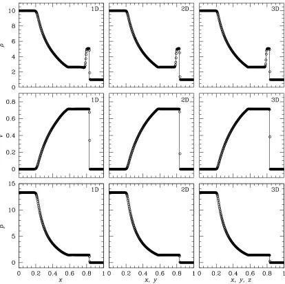
Figure 3.1(a) shows the mildly relativistic shock tube test done using 256, 2562, and
2563 cells with a Courant constant C
Cour= 0.9 and the parameters ε1,5 = 0.1 and ε2−4 = 0. The plots of one, two, and three-dimensions correspond to timest = 0.4, 0.4√2, and 0.4√3, respectively. Structures such as the shock front (at x = 0.83), contact discontinuity (at
x = 0.78) and rarefaction wave (ending at x = 0.56) are accurately produced. There are
actually slight improvements in accuracy in the multidimensional calculations. Figure 3.1(b)
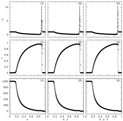
shows the highly relativistic shock tube test done again using 256, 2562, and 2563cells with a
Courant constant CCour= 0.6 and the parametersε1,5 = 0.1 andε2−4 = 0. The plots of one, two, and three-dimensions correspond to timest = 0.4, 0.4√2, and 0.4√3, respectively. The flow is more extreme, but the structure is correctly reproduced without spurious oscillations.
But in the rest mass density profile the peak does not reach the value of the exact solution
due to the coarseness of the computational cells. According to our tests, in a one-dimensional
calculation, the peak can be very accurately reproduced when 2048 numerical cells are used.
There are also improvements in accuracy in the multidimensional calculations.
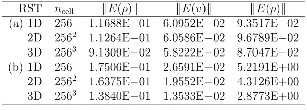
For a more quantitative comparison, we have calculated the norm errors of the rest
Table 3.1: Norm errors for the relativistic shock tube tests
RST ncell kE(ρ)k kE(v)k kE(p)k
(a) 1D 256 1.1688E−01 6.0952E−02 9.3517E−02 2D 2562 1.1264E−01 6.0586E−02 9.6789E−02
3D 2563 9.1309E−02 5.8222E−02 8.7047E−02
(b) 1D 256 1.7506E−01 2.6591E−02 5.2191E+00 2D 2562 1.6375E−01 1.9552E−02 4.3126E+00
3D 2563 1.3840E−01 1.3533E−02 2.8773E+00
kE(ρ)k=P
Figure 3.1: (a) 1D, 2D, and 3D mildly relativistic shock tube tests. The calculations have been done with the initial states in equation (3.1) using 256, 2562, and 2563 cells. The
Figure 3.1: (b) 1D, 2D, and 3D highly relativistic shock tube tests. The calculations have been done with the initial states in equation (3.2) using 256, 2562, and 2563 cells. The
3.2 Relativistic Wall Shock
A one-dimensional relativistic wall shock test has been performed in the computational
box of x = [0,1]. Initially a gas with extreme velocity occupying all numerical cells
propa-gates along the x-axis against a reflecting wall placed at x= 1. As the gas hits the wall, it
is compressed and heated and eventually a reverse shock is generated. The initial condition
of this test is
(ρ, vx, vy, vz, p) = 1,0.999999,0,0,10
−4
0≤x≤1. (3.3)
The adiabatic indexγ = 5/3 is assumed and the inflow boundary condition is used atx= 0.
This is another test which was widely used by several authors (e.g., Donat et al., 1998).
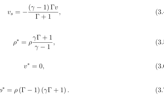
The relativistic jump condition for strong shocks with negligible preshock pressure is
given by Blandford & McKee (1976)
vs =−
(γ−1) Γv
Γ + 1 , (3.4)
ρ∗
=ργΓ + 1
γ−1 , (3.5)
v∗
= 0, (3.6)
p∗
=ρ(Γ−1) (γΓ + 1). (3.7)
Here,vsis the shock velocity and the superscript∗represents the postshock quantities, while
[image:35.612.247.531.426.599.2]the quantities without any superscript refer to the preshock gas.
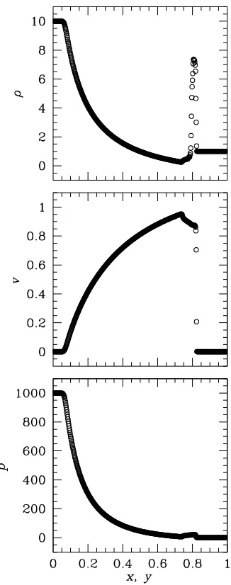
Figure 3.2 shows the structure at t = 0.75 when the reverse shock is located at x =
CCour= 0.9 and the parameters ε1,5 = 0.3 and ε2−4 = 0.1. The numerical solution is drawn with open circles and the exact solution is represented by solid lines. The numerical and
exact solutions match exactly without any oscillation or overshoot in the rest mass density,
velocity, and pressure profiles.
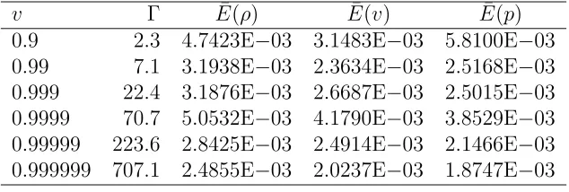
We have calculated the mean errors in the rest mass density, velocity, and pressure for
several different inflow velocities. The errors are calculated for the same time as in Figure
3.2 and given in Table 3.2. Note that the order of the mean errors is 10−3
, and that the
accuracy does not depend systematically on the investigated Lorentz factor although the
errors are smallest for the highest Lorentz factor we investigated. The mean error in the rest
mass density is.0.5% for all the Lorentz factors and about 0.25% for the maximum Lorentz
factor. This accuracy is comparable to or better than that of other published upwind scheme
Table 3.2: Mean errors for the relativistic wall shock tests
v Γ E¯(ρ) E¯(v) E¯(p) 0.9 2.3 4.7423E−03 3.1483E−03 5.8100E−03 0.99 7.1 3.1938E−03 2.3634E−03 2.5168E−03 0.999 22.4 3.1876E−03 2.6687E−03 2.5015E−03 0.9999 70.7 5.0532E−03 4.1790E−03 3.8529E−03 0.99999 223.6 2.8425E−03 2.4914E−03 2.1466E−03 0.999999 707.1 2.4855E−03 2.0237E−03 1.8747E−03
¯
E(ρ) =P
i|ρnumeri −ρexacti |/
P
3.3 Relativistic Blast Wave
The propagation of a relativistic blast wave has been tested in the two-dimensional
computational box with x = [0,1] and y = [0,1]. A gas of high density and pressure is
initially confined in a spherical region and the subsequent explosion is allowed to evolve.
This makes a spherical blast wave propagate outward. The initial condition of this test is
(ρ, vx, vy, vz, p) =
(10,0,0,0,103) 0≤p
x2+y2 ≤1/2,
(1,0,0,0,1) outside.
(3.8)
The adiabatic index is taken to be γ = 4/3 and the reflecting and outflow boundary
condi-tions are used.
The calculation was done using 5122 cells with a Courant constant CCour = 0.6 and
the parameters ε1,5 = 0.1 and ε2−4 = 0. To test the symmetry properties of the code, the calculation was stopped before a reverse shock reaches the inner reflecting boundary. Figure
3.3 shows the profiles of the rest mass density, velocity, and pressure measured along the
diagonal line connecting (0,0) and (1,1) at t = 0.7. The spherical blast wave successfully
propagates to a larger radius, and we have found that all structures in it preserve the initial
Figure 3.3: Two-dimensional relativistic blast wave test. The calculation has been done with the initial states in equation (3.8) using 5122 cells. The numerical solutions (open circles)
3.4 Relativistic Hawley-Zabusky Shock
In order to test the applicability of the code to complex relativistic flows, we have
performed a two-dimensional test simulation of the relativistic version of the Hawley-Zabusky
shock. The test was originally suggested by Hawley & Zabusky (1989) for non-relativistic
hydrodynamics. Almost the same physical values as in that original paper are used here.
Initially a plane-parallel shock with a Mach number 1.2 propagates along the x-axis into
two regions of different density. The regions are separated by an oblique discontinuity with
an inclination of 30◦
with respect to the x-axis. The density jumps three times across the
discontinuity. The initial configuration is summarized as
(ρ, vx, vy, vz, p) =
(1,0.6,0,0,0.48) 0≤x≤1/16, 0≤y≤1,
(1,0,0,0,0.48) 1/16< x ≤√3y+ 1/4, 0≤y≤1, (3,0,0,0,0.48) outside.
(3.9)
The adiabatic index γ = 1.4 is used. Inflow and outflow conditions are used at the x
-boundaries and reflecting conditions are used at the y-boundaries.
The simulation has been done in the two-dimensional computational box withx= [0,8]
and y = [0,1] using a uniform numerical grid of 2048× 256 cells. A Courant constant CCour = 0.9 and the parameters ε1,5 = 0.1 and ε2−4 = 0 were used. We have simulated this test until t = 20 in order to see the long term evolution. The passage of the planar
shock through the discontinuity causes the Kelvin-Helmholtz instability to occur along the
discontinuity and leads to the formation of vortices. The vortices roll up, interact, and
are somewhat sensitive to numerical resolution. Figure 3.4 shows the gray-scale images of
the rest mass density at different times (t = 2, 11, and 20). Because all the structures are
dragged to the right boundary as time goes on, only the left, middle, and right halves of
the computational box are shown at t = 2, 11, and 20, respectively. The vortices along
the discontinuity are clearly formed and overall the morphology is similar to that of the
3.5 Relativistic Extragalactic Jets
Finally, in order to test the applicability of the code to realistic relativistic flows, we have
simulated a two-dimensional relativistic extragalactic jet propagating into a homogeneous
medium. The relativistic jet inflows with a velocity 0.99 to the computational box ofx= [0,4]
and y = [0,1]. The jet has initially a radius of 1/8 (32 cells) and Mach number 8.76.
The density ratio of the jet to the ambient medium is 0.1 and the pressure of the jet is
in equilibrium with that of the ambient medium. The initial condition for jet inflow and
ambient medium is summarized as
(ρ, vx, vy, vz, p) =
(1,0.99,0,0,0.1) 0≤x≤1/32, 0≤y≤1/8, (10,0,0,0,0.1) outside.
(3.10)
The adiabatic index γ = 4/3 is used. The inflow and outflow conditions are used at the
x-boundaries and the reflecting and outflow conditions are used at they-boundaries.
The simulation has been done using a uniform numerical grid of 1024×256 cells with a Courant constant CCour = 0.3 and the parameters ε1,5 = 0.3 and ε2−4 = 0.1. Figure 3.5
shows the gray-scale images of logarithm of the rest mass density, pressure, and Lorentz
factor at t = 5 when the bow shock reaches the right boundary. We can clearly see the
dominant structures of bow shock, working surface, contact discontinuity, and cocoon. It
is clear that the internal structure of the relativistic jet is less complex compared to that
of a non-relativistic jet due to the effects of high Lorentz factor. The overall morphology
Figure 3.5: Two-dimensional relativistic extragalactic jet. The simulation has been carried out with the initial conditions in equation (3.10) using 1024×256 cells. Gray-scale images show logarithms of the rest mass density, pressure, and Lorentz factor (top to bottom) at t= 5, using logarithmic scales that range from−0.28 (black) to 1.98 (white) for log(density),
Chapter 4
Problem Description
We now consider the three-dimensional interactions of relativistic jets with two-phase
ambient media. These jets propagate through a denser ambient gas and then hit spherical
clouds with densities higher than that of the ambient gas. The initial ratio of the cloud
density, ρc, to the ambient medium density, ρa, and that of the beam density, ρb, to the
ambient medium density, are respectively defined as
χ≡ ρc ρa
, η≡ ρb ρa
. (4.1)
If we neglect complicating effects including radiative cooling and gravity and consider only
hydrodynamic effects, then this problem can be relatively simple and depends only on a few
hydrodynamic variables, the Mach number of the jet and the initial density contrasts given
in equation (4.1). Any geometric effects, such as different impact zone sizes or cloud shapes,
certainly will make differences in the evolutions of jets and clouds, but the overall dynamical
evolutions should not be very sensitive to them. Thus, we focus on the evolutions of jets
and clouds influenced by the above hydrodynamic effects.
The approximate propagation velocity of the jet through the homogeneous ambient
flux is ρbhbΓ
02
b v
02
b = ρahaΓ
02
av
02
a, with the following relations, v
0
b = (vb −va)/(1−vbva), Γ
0
b =
ΓbΓa(1−vbva), v
0
a = −va, and Γ
0
a = Γa. Here h is the specific enthalpy and v
0
and Γ0 represent, respectively, velocity and Lorentz factor measured in the reference frame of the
Mach disk, while v and Γ indicate those measured in the rest frame of the ambient medium.
The subscripts b and a stand for the beam and the ambient medium, respectively. After
substituting for the primed variables in terms of the unprimed ones, the conservation of the
momentum flux is derived to be
ρbhbΓ2b(vb −va)2 =ρahava2. (4.2)
Then the one-dimensional jet advance velocity, estimated in the rest frame of the ambient
medium is
va =
vb
p 1/η∗
+ 1, (4.3)
where η∗
is given by
η∗ = Γ2bρbhb ρaha
. (4.4)
In the nonrelativistic limit (h → 1, Γ → 1), η∗
approaches η, so that va represents the
classical jet advance velocity through the ambient medium, i.e., va=vb/(
p
1/η+ 1).
Based on this jet advance velocity, we define the dynamical timescale called the beam
crossing time, tbc,
tbc≡
2rc
va
, (4.5)
as the time taken for the beam to sweep a distance across the ambient medium equal to
variable va (for fixed cloud radius), it is extremely useful in comparing and characterizing
the dynamical evolutions of both jets and clouds with different model parameters.
Although we use the beam crossing time as the primary timescale in this study, it is
also interesting to estimate the cloud crushing and cooling timescales. The cloud crushing
timescale is the time required for the beam to cross the cloud diameter during the phase
of cloud compression, and if va is nonrelativistic, this timescale can be approximated as
tcc ∼2√χrc/va(Klein et al., 1994). Clearly, tbc'tcc in the absence of clouds, and for dense
clouds (χ1), tbc< tcc. Following Fragile et al. (2004), the cloud cooling timescale can be
roughly estimated fromtcool ∼Cv3a/(χ3/2ρc), where the constant C = 7.0×10⁻³⁵ g cm−6 s4.
With values reasonable for kpc-scale extragalactic situations, rc= 1 kpc, va = 0.1c,χ= 100,
and ρc = 102mH cm
−3
, we find that tbc < tcc ∼ tcool. Thus cooling will not be extremely
important during the cloud compression phase for the chosen values. For fixed density and
cloud radius, the cloud cooling timescale becomes longer compared to the cloud crushing
timescale as va increases, so the effect of cooling is somewhat reduced for relativistic jets
compared to nonrelativistic ones. For parameters more relevant to VLBI-scale jet/cloud
collisions, rc= 0.5 pc, va = 0.5c, χ= 104, and ρc = 106mH cm
−3
, we have tbc ∼ tcool < tcc,
so cooling would be more important in this case. A more detailed consideration of cooling
timescales is beyond the scope of this study.
Three distinct evolutionary stages can be considered in this problem. There is an initial
jet propagation stage where the jet advances through a homogeneous ambient medium with
cloud/ambient density contrast is sufficiently large and the jet speed is relatively slow, the
speed of the transmitted shock in the cloud is much slower than that of the bow shock of the
jet. Thus the bow shock entirely encloses the cloud, which leads to the development of the
Kelvin-Helmholtz instability at the cloud surface (e.g., Klein et al., 1994). The final stage
is when the jet passes through the cloud. In this phase the cloud begins to reexpand just
after the jet reaches the rear edge of the cloud. At the same time, the jet propagates in the
original direction if it has dominated the cloud or in a new direction if the cloud was massive
Chapter 5
Numerical Simulations
5.1 Basic Equations
The special relativistic hydrodynamic equations are written in a covariant form (e.g.,
Landau & Lifshitz, 1959; Wilson & Mathews, 2003)
∂α(ρUα) = 0, (5.1)
∂αTαβ = 0, (5.2)
where the energy momentum tensor is given by
Tαβ = (e+p)UαUβ +pgαβ. (5.3)
Here, ∂α =∂/∂xα is the covariant derivative with spacetime coordinates xα = [t, xj], Uα =
[Γ,Γvj] is the normalized (UαUα = −1) four-velocity vector, and a metric tensor gαβ with
a signature +2 is used. The mass density, velocity, internal plus mass energy density, and
pressure in the local rest frame are denoted by ρ, vj, e, and p, respectively. Greek indices
(e.g., α, β) denote the spacetime components while Latin indices (e.g., i, j) indicate the
For our numerical purposes, it is convenient to rewrite the covariant equations (5.1)–
(5.3) in the index form which gives a hyperbolic system of conservation equations
∂D ∂t +
∂ ∂xj
(Dvj) = 0, (5.4)
∂Mi
∂t + ∂ ∂xj
(Mivj +pδij) = 0, (5.5)
∂E ∂t +
∂ ∂xj
[(E+p)vj] = 0, (5.6)
where the equation of state (EOS) is given by
p= (γ−1) (e−ρ). (5.7)
Here, D, Mi, and E are the mass density, momentum density, and total energy density in
the reference frame, respectively, and γ is the adiabatic index. We note that we restrict
ourselves to an ideal gas EOS in this study although future expansions of this work could
use a more general EOS (e.g., Ryu et al., 2006).
The quantities in the reference frame are related to those in the local rest frame via
following transformations
D= Γρ, (5.8)
Mi = Γ2(e+p)vi, (5.9)
where the Lorentz factor is given by
Γ = √ 1
1−v2 (5.11)
with v2 =v2
x+vy2+vz2.
If an EOS is assumed, the local sound speed, cs, and the specific enthalpy, h, are easily
derived. For an ideal gas, they are given by
c2s = 1 h
∂p ∂ρ +
∂p
∂e, h= 1 + γ γ−1
p
ρ. (5.12)
A γ-law gas such as an ideal gas has the local sound speed limit cs ≤√γ−1. Only in the
ultrarelativistic case,eρ, does the local sound speed approach its limit (i.e.,cs →√γ −1).
5.2 Numerical Method and Setup
The system of equations (5.4)–(5.7) can be solved numerically with explicit finite
dif-ference upwind schemes which are based on exact or approximate Riemann solvers using
the characteristic decomposition of these relativistic hydrodynamic conservation equations.
Although the upwind schemes were originally developed for nonrelativistic hydrodynamics,
some schemes have been extended to special relativistic hydrodynamics while retaining the
advantages of the upwind schemes, including high accuracy and robustness.
We use the multidimensional code for solving the special relativistic hydrodynamic
is an explicit Eulerian finite difference upwind scheme and an extension of the Roe scheme
to second-order accuracy in space and time. Our code uses a new set of conserved
quanti-ties, which lead to a new eigenstructure for special relativistic hydrodynamics and employs
an analytic formula for the calculation of the local rest frame quantities from the reference
frame quantities. The advantage of our code is that it is simple and fast, and yet it is
ac-curate and reliable enough. The performance of the code was demonstrated through several
standard tests, including relativistic shock tubes, a relativistic wall shock, and a
relativis-tic blast wave, as well as test simulations of the relativisrelativis-tic version of the Hawley-Zabusky
shock and a relativistic extragalactic jet given in Chapter 3. For our new simulations, we
have parallelized this code using the message-passing interface (MPI) and this parallelized
version is given in the Appendix. The simulations described here typically use 64 processors
on a Linux cluster.
Table 5.1 lists the initial parameters of the four different relativistic jet-cloud interaction
models we have investigated in this study. All models use the adiabatic index γ = 4/3 and
assume pressure-matched jets and clouds, i.e.,pb/pa=pc/pa= 1, wherepb,pc, andpaare the
pressure of the beam, cloud, and ambient medium, respectively. We set c=rc =ρa ≡1 in
our models, so that all physical quantities are dimensionless and can be scaled to any specific
physical model (e.g., t → tc/rc, ρ → ρ/ρa). The initial Newtonian beam Mach number,
MN
b ≡ vb/cs,b, where cs,b is the sound speed in the beam, as well as the initial relativistic
beam Mach number, MR
b ≡ (Γb/Γs,b)MNb , where Γs,b is the Lorentz factor associated with
the beam sound speed are given in Table 5.1. As discussed in K¨onigl (1980), in the context
of relativistic gasdynamics the relativistic Mach number is the best analog of the Newtonian
physical properties in our models. The initial density contrast between the beam and the
ambient medium is fixed to η = 0.1, so that jets strike clouds with densities 100 to 1000
times higher than the initial beam density. While even smaller values of η would have been
more realistic for most extragalactic jets, they lead to extremely short time steps when the
jets strike the clouds, making them computationally unachievable. Previous studies have
indicated that most important properties for fast jets are relatively insensitive to values of
η.0.1 (e.g., Rosen et al., 1999). In models M1 and M2, the clouds interact with the lower
relativistic beam Mach number jets, so the relativistic effects are less dominant, with smaller
beam velocities and internal energies. Model M1 is identical to model M2 except for the
smaller density ratio of the cloud to the ambient medium. Models M3 and M4 have been
chosen to study the cloud interactions with jets with higher relativistic beam Mach numbers,
which have more dominant relativistic effects caused by larger beam velocities and internal
energies. Again, the initial conditions of model M3 are the same as those of model M4 except
for the smaller density ratio of the cloud to the ambient medium.
We set up the density gradient of the spherical cloud edge with a hyperbolic tangent
function
ρ(r) = ρc+ρa
2 +
ρc−ρa
2 tanh
rc−r
∆r
, (5.13)
where r is the distance from the center of the cloud and ∆r is the scale parameter for
the width of density transition (∆r rc). The presence of a true density discontinuity
instead of this steep function would not affect the actual dynamics of jet-cloud interactions
other physical quantities such as pressure and velocity are constant across the transition
width.
The simulations have been performed in the three-dimensional computational domain
with x = [0,8], y = [0,8], and z = [0,8] using a uniform Cartesian grid of 2563 cells.
The beam, with a circular cross section of radius rb = 1/4 (8 cells), is initially located
at (x, y, z) = (0,4,4) and propagates through the ambient medium along the positive x
-direction. In order for the relativistic jet to collide off axis with the cloud at rest, the center
of the cloud, with radius rc = 1 (32 cells), is placed at (x, y, z) = (4,3.5,4); hence the
relativistic jet hits the spherical cloud with an impact angle of 30◦
. The outflow boundary
condition is imposed on all boundaries of the computational domain except where the inflow
boundary condition is used to maintain the continuous jet. We were able to assign the
relativistic jet only 8 cells per initial beam radius and the cloud 32 cells per initial cloud
radius due to the limitation of computational resources. This resolution is less than that
of previously reported two-dimensional works which are related to this problem. Thus our
three-dimensional simulations may not be fully converged and some quantities to be described
may change if three-dimensional simulations with much higher resolutions can be performed
in future studies; however, our tests of the code do indicate that simulations with this level
Table 5.1: Simulation parameters
Model χ η vb Γb MNb MRb tbc tend
M1 10 0.1 0.9 2.29 2.92 6.36 4.86 4tbc
M2 100 0.1 0.9 2.29 2.92 6.36 4.86 6tbc
M3 10 0.1 0.99 7.09 1.92 11.6 2.50 4tbc
M4 100 0.1 0.99 7.09 1.92 11.6 2.50 5tbc
Here χ is the ratio of the cloud density to the ambient medium density, ηis the ratio of the beam density to the ambient medium density, vb is the initial beam velocity,
Γb is the beam Lorentz factor, MNb is the Newtonian
beam Mach number, MR
b is the relativistic beam Mach
number, tbc is the beam crossing time, and tend is the
Chapter 6
Results
6.1 Morphology and Dynamics
The gray-scale images in Figures 6.1(a)–(d) show the distinct evolutionary phases of
models M1–M4, respectively. These images show the x−y plane with z = 4 in the three-dimensional computational domain, thus providing a slice through the center of the jet and
cloud. In each of these figures the top to bottom panels represent density, pressure, and
Lorentz factor, respectively (in logarithmic scales) while the left to right panels represent
evolutionary stages shown at three different times, t=tbc, (tbc+tend)/2, and tend.
The early stages of the relativistic jet propagation through the uniform ambient medium
until the jet is about to collide the cloud (t/tbc ∼ 1) are basically similar to those found
in earlier simulations (e.g., Mart´ı et al., 1997; Aloy et al., 1999b). Several key features are
clear from the left panels of Figures 6.1(a)–(d). In all the models a bow shock that separates
the jet from the external medium is driven, the beam itself is terminated by a Mach disk
(terminal shock) where most of the beam kinetic energy is converted into its internal energy,
and shocked jet material flows backward into a cocoon within the contact discontinuity that
separates the shocked external gas and the shocked jet gas. There is no difference between
models M1 and M2 and between models M3 and M4 at this stage because of the same
initial conditions of the jets and the same ambient media properties for these two pairs of
The relativistic beam Mach number of the jet is associated with the shape of the bow
shock. In models M1 and M2, the lower relativistic beam Mach number jets, with a lower
propagation velocity (va ∼0.42) and internal energy, have bow shocks with narrower conical
shapes, and the Mach disk is quite close to the bow shock. This conical shape of the bow
shock tends to be broader as the relativistic beam Mach number of the jet increases, as
seen for models M3 and M4; these higher relativistic beam Mach number jets, with a higher
propagation velocity (va ∼ 0.78) and internal energy, also have the Mach disk standing off
farther from the bow shock. The shapes of the bow shocks are also connected with the sizes
of the impact cross section when the jets begin to interact with the cloud. The low relativistic
beam Mach number jets in models M1 and M2 feature relatively thick cocoons while the
high relativistic beam Mach number jets in models M3 and M4 have thinner cocoons. This
dependence of the cocoon morphology on the relativistic beam Mach number is consistent
with previous results (see e.g., Mart´ı et al., 1997). Although the structural differences in the
jet head and the cocoon are evident by this early stage of the evolution, internal structures
within the beam and backflows are not yet dominant and are barely distinguishable at this
stage.
In every model, the relativistic jet begins to partially deflect as a direct response to its
interactions with the clouds. This is seen in the middle column of panels of Figures 6.1(a)–
(d), and most clearly visible in the middle bottom panels where fast streams emerge from
the Mach disk at significant angles with respect to the jet axis. These deflection features are
these angles peak when the jets cross over approximately half the clouds (at t/tbc ∼ 2.5,
3.5, 2.5, and 3 for models M1–M4, respectively). For these comparable dynamical times,
models M2 and M4, both with χ = 100 but having different beam Mach numbers, show
80◦
−90◦
deflection angles, while models M1 and M3, with the same beam Mach numbers
as the models M2 and M4, respectively, but with χ= 10, show smaller deflection angles of
about 45◦
. This indicates that the deflection angle is more strongly influenced by the density
contrast, χ, than by the beam Mach number of the jet. For an off-axis collision there are
weak deflection features on the other side of the jet axis, where the deflection of the outflow
from the beam is significantly suppressed by the dense cloud. That suppression leads to the
production of a strong oblique shock within the beam. As seen in the figures, the oblique
shocks are quite strong in models M2 and M4, but in models M1 and M3 there are only
relatively weak oblique shocks in the beam. Comparing at this stage models M1 and M3
with models M2 and M4, we note that the bow shocks enclose less of the cloud in models
M1 and M3 because of their lower density contrast, χ. That implies quicker penetration of
the clouds by these jets, so the strengths of the oblique shocks in these beams are reduced.
Some additional properties of the simulations at this stage are shown in Figures 6.2
and 6.3. Figure 6.2 illustrates one-dimensional flow structures of density, pressure, and
Lorentz factor along the beam propagation axis for models M1 and M3 at the same epochs
as in Figures 6.1(a) and (c). In both models there are spikes in the density and pressure
associated with the impact by the incident jets, while there is little change in beam Lorentz
factor. Figure 6.3 shows the images of the logarithm of the Lorentz factor projected at
the viewing angle of 0◦
for models M2 and M4, at t/tbc = 3.5 and 3, respectively. These
gas induced by the jet. This gas is an admixture of jet and cloud material, but only a small
fraction of the cloud gas is shown in these projection images since the mean cloud velocity
computed in each component (refer to Section 6.2) is hvii . 0.01 and 0.06 for models M2
and M4, respectively, at the same epoch as in Figure 6.3. This implies that this deflected
gas consists predominantly of jet material although small amounts of cloud material are
entrained in these deflected structures. This presence of deflected gas accelerating toward a
terminal velocity strongly suggests that such deflected and accelerated gas is responsible for
at least some of the outflowing gas observed in the vicinity of AGNs.
Once the jet passes through the cloud, it begins to accelerate, causing a change in the
shape of the bow shock. As visible in the right panels of Figures 6.1(a)–(d) shown when the
jet head nearly reaches the boundary of the computational cube (att/tbc = 4, 6, 4, and 5 for
models M1–M4, respectively), the shapes of the bow shocks change more clearly in the low
relativistic beam Mach number jets than in the high relativistic beam Mach number jets.
That reflects the fact that the acceleration of the jets is somewhat faster in low relativistic
beam Mach number jets. That reacceleration occurs in essentially the original propagation
direction or in a somewhat new direction. In our simulations there is a trend for the flow
of the jet to be bent more when a lower relativistic beam Mach number jet interacts with a
denser cloud, with the least bending seen for model M3 and the most for model M2. We see
in the right panels of Figure 6.1(b) that the beam is bent by about 10◦
with respect to the
original jet axis. The bent jet still remains stable and collimated over the several dynamical