Deterministic mutation algorithm as a winner over forward selection procedure

DETERMINISTIC

MUTATION

ALGORITHM

AS

A

WINNER

OVER

FORWARD

SELECTION

PROCEDURE

Md Fahmi Abd Samad

Optimization, Modeling, Analysis, Simulation and Scheduling Research Group, Centre for Advanced Computing Technology, Universiti Teknikal Malaysia Melaka, Durian Tunggal, Melaka, Malaysia

Faculty of Mechanical Engineering, Universiti Teknikal Malaysia Melaka, Durian Tunggal, Melaka, Malaysia E-Mail: [email protected]

ABSTRACT

System identification is a field of study involving the derivation of a mathematical model to explain the dynamical behaviour of a system. One of the steps in system identification is model structure selection which involves the selection of variables and terms of a model. Several important criteria for a desirable model structure include its accuracy in future prediction and model parsimony. A parsimonious model structure is desirable in enabling easy control design. Two methods of model structure selection are closely looked into and these are deterministic mutation algorithm (DMA) and forward selection procedure (FSP). The DMA is known to be originated from evolutionary computation whereas FSP may be listed under the study of regression. They have close similarities in characteristics, more specifically known as forward search in model structure selection. However, both also function in a population-based optimization and statistical approaches, respectively. Due to the closeness, this research attempts to clarify the advantages and disadvantages of both methods through model structure selection of difference equation model in system identification. Simulated and real data were used. To allow for fair comparison, DMA was altered so as to equalize its strength, where applicable, to that of FSP. In the real data simulation, both methods obtained the same model structure whereas in simulated data modelling, only DMA was able to select the correct model structure. This concludes that DMA not only has the advantage of simpler procedure but it also superseded the performance of FSP, even with a handicapped alteration.

Keywords: system identification, model structure selection, deterministic mutation algorithm,forward selection procedure.

INTRODUCTION

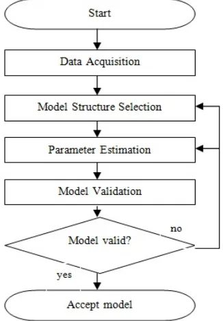
System identification is a method of determining a mathematical model for a system given a set of input-output data of the system (Johansson, 1993). There are four main steps involved in system identification and these are data acquisition, model structure selection, parameter estimation and model validation, shown in Figure 1 (Söderström and Stoica, 1989, Ljung, 1999). As one of the stage in system identification, the model structure selection stage refers to the determination of the variables and terms to be included in a model. Basically, an optimum model is described as having adequate predictive accuracy to the system response yet parsimonious in structure. A parsimonious model structure is preferred since, with less number of variables and/or terms, system analysis and control becomes easier.

With the continuous demand for an efficient method of model structure selection, two algorithms are looked into in more detail in order to search for a more efficient method. These two methods are deterministic mutation algorithm (DMA) (Abd Samad et al. 2011) and

forward selection procedure (FSP) (Draper and Smith, 1998). DMA is known to be an alteration from well-known evolutionary computation alternatives. It functions as an optimization for a population of solutions. On the other hand, FSP is one of the methods commonly found under the study of regression and relies heavily on statistical distribution analysis. They have close similarities in characteristics, more specifically known as forward search in model structure selection. Due to the closeness, this research attempts to clarify the advantages

and disadvantages of both methods through model structure selection in system identification. Such attempt is carried out by comparing the application of both methods to model structure selection of difference equation model, particularly based on model accuracy and parsimony.

METHODOLOGY

Forward selection procedure

FSP attempts to achieve a similar conclusion as backward elimination (Draper and Smith, 1998). Another name used for the procedure is stepwise forward inclusion. It evaluates variables one at a time and has also been used with orthogonal least squares-error reduction ratio method (Mendes and Billings, 2001). The backward elimination begins with the largest regression, using all variables, and subsequently reduces the number of variables in the equation until a decision is reached on the equation to use. Forward selection does this by working from the other direction, which is to insert variables in turn until the regression equation is satisfactory. The order of insertion is determined by using the partial correlation coefficient as a measure of the importance of variables not yet in the equation. The basic procedure is as follows (assume X as input and Y as output):

(i) Select the X most correlated with Y (suppose it is X1) and find the first-order, linear regression equation in the form of _Yˆ_{ f ( X )1 .}

(ii) Find the partial correlation coefficient of Xj (j1) and Y (after allowance for X1). Mathematically, this is equivalent to finding the correlation between (a) the residuals from the regression _Yˆ _{ f ( X )1 and (b) the} residuals from a regression _Xˆ _{f ( X )1}

j j (which has not actually been performed).

(iii) Select Xj with the highest partial correlation coefficient with Y (suppose this is X2) and fit a second regression equation _Yˆ _{ f ( X , X1 2)}

(iv) Repeat the process as in (ii) and (iii).

After X1, X2,…, Xq are in the regression, the partial correlation coefficients are the correlations between (a) the residuals from the regression

1 2 ˆ

Y f ( X , X ,..., X_q) and (b) the residuals from a

regression of _Xˆ _{f ( X , X ,...X1 2 )( j q )} q

j  j 

As each variable is entered into the regression, the following values are examined:

(i) R2_{, the multiple correlation coefficient;}

(ii) The partial F-test value for the variable most recently entered, which shows whether the variable has taken up a significant amount of variation over that removed by variables previously in the regression. As soon as the partial F value related to the most recently entered variable becomes insignificant the process is terminated. The variable recently entered is not included in the final model and dropped out. The parameter estimation method is least squares.

The partial F-test determines when to stop the insertion. This is carried out every time a new regression equation is built. One may see that FSP requires multiple measurements and a threshold to determine significance. In Kleinbaum et al. (2008), an alternative parameter is calculated which is p-value. It is related to partial F value such that large partial F value indicates small p-value.

Deterministic mutation algorithm

In Abd Samad et al. (2011), the development of

DMA takes advantage of the knowledge that the inclusion of more regressors to a model decreases the prediction error gradually, provided that no overfitting occurs (Draper and Smith, 1998). In order to achieve this, DMA operator is designed to be deterministic. Consequently, the problem of determining suitable operator probabilities is avoided. Operators with deterministic feature have been used together with evolutionary computation for trajectory optimization (Kanarachos et al. 2003) and model

parameter estimation (Koulocheris et al. 2004, Dertimanis

et al. 200).

The operator of DMA is characterized by its past performances to enable quicker detection of parsimonious models. The algorithm is an original adaptation of evolutionary computation with no crossover and the characteristic of a forward search. DMA contains a specific rule that dictates whether the genetic operation is to be implemented or not. The algorithm’s search is based on generational evaluation of schemata followed by the evaluation of the best schema’s subset in coherence with the implicit parallelism theory introduced in Holland (1992). The pseuducode is provided as in Figure-2.

> procedure DMA

> begin

> t = 1

> initialize P(t) with chromosomes

of only 1 gene of allele 1

> evaluate P(t)

> while (P(t) > 1 chromosome) do

> begin

> t = t + 1

> identify the critical gene

from the best chromosome

> construct P(t) from P(t -

1) by removal of the best

chromosome

> operate on P(t) with

deterministic mutation

> evaluate P(t)

> end

> end

Figure-2. Pseudocode for DMA.

the following objective function (OF) is used (Ljung, 1999):

2

ˆ ( ( ) ( )) N

t k

OF y t y t







where y tˆ

 

and actual output value at time t, respectively, and N is the

number of data. The k-step-ahead prediction is used when

the value of k depends on output smallest lag order.

SIMULATION

A simulation study was conducted using numerical software to compare the performance of FSP and DMA in system identification. The data acquisition stage was made by using a real data known as Hald Data where the correct structure is unknown. The next data comes from a simulated nonlinear autoregressive with exogenous variable (NARX) model. The simulated model assumes time delay = 1. Simulated model was used to

enable direct comparison of the correct solution to the solution found by different methods. This is possible by knowing the sequence of regressor selection in the computer program.

RESULTS AND DISCUSSION

Hald data modelling

The Hald data is a well-known real data used to demonstrate the effectiveness of regression methods (Draper and Smith, 1998). According to Draper and Smith (1998), it was given in Hald (1952) and originated from Woods et al. (1932). It contains 13 sets of data where each

set consists of 4 input variables commonly labelled X1, X2, X3 and X4 and 1 output variable Y.

Table-1 shows the sequence of variable selection and statistical data using FSP. The result is actually coherent with the findings in Draper and Smith (1998) taking note on the sequence of insertion.

Table-1. Result of variable selection for Hald system identification using FSP.

As opposed to FSP, DMA does not work by including a constant term since the beginning of

modelling. The original approach is to let the algorithm decide whether an inclusion of a constant term is necessary (compulsory) or not. The results of modelling of Hald data by letting DMA decide on the need for constant term inclusion is shown in Table-2. Maximum number of regressors was used as its termination criterion. The simulation shows that DMA identifies the constant term to be the most significant term that should be included in the model.

DMA may also be applied to assume that a constant term may not be needed at all. The result of this variant is in Table-3.

Another variant is also created for modelling using DMA. The approach is to always include a constant term as is the case with FSP. The result is the same as when the constant term was not purposely added in (Table-2).

Table-2. Result of variable selection for Hald system identification using DMA (Constant term is not

compulsory).

Table-3. Result of variable selection for Hald system identification using DMA (Constant term is absent).

Figure-3. Multiple correlation coefficient vs number of variables using different methods for hald data.

Simulated data modelling

NARX model is a common model structure representation for nonlinear discrete-time system, uses reasonably small number of regressors and is also a generalisation of the linear difference equation. The following is the model, to be identified, written as linear regression models, its specification, number of correct regressors out of its maximum regressors and size of search space:

2

( ) 0.5 ( 1) 0.3 ( 2) 0.3 ( 1) ( 1)

0.5 ( 1) ( )

y t

y t

u t

y t

u t

u t

e t



 

 







 

Specification: nonlinearity = 2, lag order of output = 1, lag order of input= 2;

Number of correct regressors: 4 out of maximum 10 including a d.c. level (constant);

Search space: 1023 possible models

The input u(t) was generated from random

uniform distribution in the interval [-1,1] to represent white signal while the noise e(t) was generated from

random uniform distribution [-0.01,0.01] to represent white noise. Five hundred data points were generated from the model. As the number of data points increases, all models are found to be ergodic i.e. any sample can be assumed to have a fixed mean and standard deviation.

The results of modelling the simulated model using FSP is shown in Table-4. By looking at the table and comparing back to the original model, it is seen that the method was late in identifying one of the variable as a significant variable. The variable y(t-1)u(t-1) was

identified as significant at step 5, and instead it identified a different variable i.e. u(t-1) that was not in the model to be

significant.

Table-4. Result of variable selection for simulated system identification using FSP.

The DMA approaches as adopted earlier for Hald data were here repeated for modelling of the simulated data. The result when DMA decides whether the inclusion of a constant term is necessary or not is as in Table-5. In this simulation, the algorithm actually decides that the constant term is not necessary. Its inclusion, as in step 10, does no significant improvement to the R2 _value.

Table-5. Result of variable selection for simulated system identification using DMA (Constant term is not

compulsory).

Table-6. Result of variable selection for simulated system identification using DMA (Constant term is compulsory).

By comparing the results from these 3 approaches for the simulated data, one observed that the sequences of variable inclusion are different even from the beginning. Interestingly, DMA was able to obtain the correct model structure by identifying that the constant term is not necessary and with the inclusion of the 4 correct variables/terms at generation 4. Table-7 shows the R2 values for the approaches while Figure-4 shows the plot. The graph shows that DMA is always better than FSP, even by including a constant term.

Table-7. Multiple correlation coefficient vs number of variables and constant term using different methods.

Figure-4. Multiple correlation coefficient vs number of variables and constant term using different methods for

simulated data.

CONCLUSIONS

A well-known regression method, commonly known as FSP has been compared to a method that originated from EC for model structure selection. FSP has rather heavy statistical computation. On the other hand, the EC method, known specifically as DMA has less computational requirement. Both methods have very strong similarities i.e. forward search where a variable/term is included into a model one by one. Furthermore, to allow for a fair comparison, DMA was altered so that there are 2 variants – one which purposely include a constant term and one which decides on the inclusion.

Both methods were applied to two sets of data – Hald data and a simulated NARX model data. In Hald data, both methods (and the variants) perform equally as each variable was entered.

In simulated data modelling, DMA performed better by not including a constant term. In addition to that, when a constant term is forced into the model, DMA also was able to show better performance than FSP. In both variants of DMA, the correct regressors were able to be identified as opposed to FSP.

ACKNOWLEDGEMENTS

Thanks to UTeM for grant PJP/2012/FKM(20C)/S01117

REFERENCES

[1] Abd Samad, M. F., Jamaluddin, H., Ahmad, R., Yaacob, M.S. and Azad, A. K. M. (2011) Deterministic Mutation-Based Algorithm for Model Structure Selection in Discrete-Time System Identification. International Journal of Intelligent Control and Systems, 16(3), pp. 182-190.

International Congress on Computational Mechanics. June 29-July 1. Limassol, Cyprus: GRACM, 1, pp. 395-402.

[3] Draper, N. R. and Smith, H. (1998). Applied Regression Analysis (3rd _{ed.), New York: John Wiley} and Sons, Inc.

[4] Hald, A. (1952). Statistical Theory with Engineering Applications, New York: Wiley.

[5] Holland. J. H. (1992). Adaptation in Natural and Artificial Systems (MIT Press ed.), Massachusetts Institute of Technology (1975) (1st _{ed.), The} University of Michigan.

[6] Johansson, R. (1993). System Modeling & Identification, Englewood Cliffs, New Jersey: Prentice-Hall, Inc.

[7] Kanarachos, A, Koulocheris, D. and Vrazopoulos, H. (2003). Evolutionary Algorithms with Deterministic Mutation Operators Used for the Optimization of the Trajectory of a Four-Bar Mechanism. Mathematics and Computers in Simulation, 63(6), pp. 483-492.

[8] Kleinbaum, D.G., Kupper, L.L., Nizam, A. And Muller, K.E. (2008). Applied Regression Analysis and Other Multivariable Methods (4th _{edition), California:} Thomson Higher Education.

[9] Koulocheris, D., Dertimanis, V. and Vrazopoulos, H. (2004). Evolutionary Parametric Identification of Dynamic Systems. Forschung im Ingenieurwesen, 68(4), pp. 173-181.

[10] Ljung, L. (1999). System Identification: Theory for the User (2nd _{ed.), Upper Saddle River, New Jersey:} Prentice Hall PTR.

[11] Mendes, E. M. A. M. and Billings, S. A. (2001). An Alternative Solution to the Model Structure Selection Problem. IEEE Transactions on Systems, Man and Cybernetics - Part A: Systems and Humans, 31(6), pp. 597-608.

[12] Söderström, T. and Stoica, P. (1989). System Identification, London: Prentice Hall International (UK) Ltd.