A Note on Ratio Estimators in two Stage Sampling

(1)

A Note on Ratio Estimators in two Stage Sampling

Sitanshu Shekhar Mishra

Lecturer in Statistics, Trident Academy of Creative Technology (TACT), Bhubaneswar, Odisha, India.

Abstract- In this paper a number of ratio estimators in two stage sampling are considered and their efficiencies are compared with an estimator without use auxiliary information. Numerical illustration is provided to compare the efficiencies.

I. INTRODUCTION

n large scale sample surveys it is usual practice to adopt multi stage sampling to estimate the population mean or total of the study variable y. The main purpose of using multi stage sampling in place of unrestricted unistage sampling is to reduce the cost of

survey operations even if estimates derived from multi stage sampling are likely to be less efficient then those of the unrestricted uni-stage sampling. Sometimes, all auxiliary variable x compared with y may be available either at primary stage or of secondary stage or at both the stages to in case the efficiency of estimate of the finite population parametric functions such as population means or total. Thus, in the following we consider different ratio estimators of population mean of the study variable y in two –stage sampling using knowledge on a single auxiliary variable x.

II. NOTATIONS

Now, consider a finite population U partitioned into N first stage units (fsu) denoted by U1, U2, ……UN. Let Mi be the number

of second stage units in

U (i

i



1, 2,...., N)

_{. Define}

N i i 1

M



_

and

N i i 1

1 M

M

N



_

. Let

y

ij_and

x

ij_{denote values of the}

study variable y and the auxiliary variable x respectively for the jth ssu of Ui = (j = 1, 2, …, Mi, i= 1, 2, ….,N) .

Define,

i

M i ij

j 1 i

1 Y

y

M



_

and

i

M i ij

j 1 i

1 X

x

M



_

(i = 1, 2, ….., N)

The population mean of y,

N i i i 1

1 Y

u Y

N





and the population mean of x,

N i i i 1

1 X

u X

N



_

, where

i i

M

u

M



.

Further, define

Y

R

X



and

i i

i

Y

R

X



(i = 1, 2, ….., N)





N ₂

2

by i i i 1

1 S

u Y

Y

N 1



 









N ₂

2

bx i i i 1

1 S

u X

X

N 1



 











N

bxy i i i i i 1

1 S

u Y

Y u X

X

N 1



 









i

M ₂

2

iy ij i j 1

i

1 S

y

Y

, i

1, 2,..., N.

M

1















i

M ₂

2

ix ij i j 1

i

1 S

x

X

, i

1, 2,..., N.

M

1











(2)







i

M

ixy ij i ij i j 1

i

1 S

x

X

y

Y ,

M

1







i = 1, 2, …, N.

Define,

i

m i ij ij

j s j 1

i i

1

1 y

y

m



m



_



_

i

m i ij ij

j s j 1

i i

1

1 x

x

m



m



_



_

n i i i i i s i 1

1

1 y

u y

n



n









n i i i i i s i 1

1

1 x

u x

n



n



_



_





n ₂

2

by i i i 1

1 s

u y

y

n 1



 









n ₂

2

bx i i i 1

1 s

u x

x

n 1



 











n

bxy i i i i i 1

1 s

u y

y u x

x

n 1



 









i

m ₂

2

iy ij i j 1

i

1 s

y

m

1











i

m ₂

2

ix ij i j 1

i

1 s

x

m

1













i

m

ixy ij i ij i j 1

i

1 s

y

x

m

1







bxy ixy

b i

by bx iy ix

S

,

S S



 

 

(i = 1, 2, ….,N)

by bx

bx by

S

C

, C

X

Y





iy ix

ix iy

i i

S

C

, C

,

X

Y



(i = 1, 2, …., N)

III. RATIO ESTIMATORS

Consider the following ratio type estimators under two-stage sampling scheme.

n 0 i i

i 1

1 T

u y ,

n





without using auxiliary information on x.

n i i i 1 1 n

i i i 1

1 u y

n

T

X.

1 u x

n





(3)

n i 2 i i

i 1 i

1 y

T

u

X

n



x



_

n i i i 1 3 n

i i i 1

1 u y

n

T

X,

1 u X

n





Smith (1969)

n i i i i 1 _i 4 _n

i i i 1

1 y

u

X

n

x

T

X

1 u X

n





, Murthy (1967)

n

i ii n i 1

5 _n i i i 1 i i i 1

1 u y

1 n

T

u X

1 _n

u x

n



 





These estimators belong to the class of estimators considered by Panda (1998).

T1 requires advance knowledge on j

X

T2 and T5 require advance knowledge on

X (i

i



1, 2,...., n)

; T3 and T4 require advance

knowledge on

X

and

X i

i





1, 2,..., n



_.

IV. BIASES AND MEAN SQUARE ERRORS OF ESTIMATORS

As known, T0 is an unbiased estimator of

Y

. T1, T2, T3, T4, and T5 are biased estimates of

Y

and upto

1

0 n

 

 

 

_{, the biases are} :

2 2

bxy 2 ixy

bx ix

1 2 i 2

i i

S

1

1 S

B(T )

Y

u

n

N

X

Y X

nN

m

M

X

Y X





_

_



















_

_



_

_



_



_



_

_



_

_





















2 N

ixy ix

2 i i 2

i 1 _i _i _i _i _i

S

1

1 S

B(T )

u Y

N



m

M

X

X Y









_



_



_









2

bxy bx

3 2

S

1

1 B(T )

Y

n

N

X

Y. X













_



_{ }



_



 



2 _n 2 _n

bxy ixy

bx ix

4 2 i i 2 i i

i 1 i 1

i i i i i i

S

1

1 S

1 B(T )

Y

COV

u Y

,

u X

n

N

X

X Y

n



m

M

X

X Y

n



























_



_

_



_



_

_



_



_

_



_{ }

_

_



_

_

_



_

2 _N 2

ixy 2

bx ix

5 2 i 2

i 1 _i _i

S

1

1 S

B(T )

Y

u

n

N X

nN



m

M

X

Y. X





















_

_



_



_



_

_



_

_



















To

1

0 n

 

 

 

_{the mean square errors (MSE) of T}₁_{, T}₂_{, T}₃_{, T}₄_{and T}₅_{are given by}

MSE(T0)

N

2 2 2

by i iy

i 1 _i _i

1

1 S

u

S

n

N

nN



m

M







_{ }



_



_



_



_

(4)





N

2 2 2 2 2 2 2

1 by bx xy i iy ix ixy

i 1 _i _i

1

1 MSE(T )

S

R S

2RS

u

S

R S

2RS

n

N

nN



m

M







_{ }

_

_

_



_



_{ }





_



_



_











_

_





N

2 2 2 2 2

2 by i iy i ix i ixy i 1 _i _i

1

1 MSE(T )

S

u

S

R S

2R S

n

N

nN



m

M







_{ }



_



_



_



_











_

_

N

2 2 2 2 2

3 by bx xy i iy

i 1

i i

1

1 MSE(T )

S

R S

2RS

u

S

n

N

nN



m

M







_{ }

_

_

_



_



_{ }





_



_



_











N

2 2 2 2 2 2 2

4 by bx yx i iy i ix i ixy

i 1 _i _i

1

1 MSE(T )

S

R S

2RS

u

(S

R S

2R S )

n

N

nN



m

M







_{ }

_

_

_



_



_{ }





_



_



_











_

_

N

2 2 2 2 2

5 by i iy ix ixy

i 1

i i

1

1 MSE(T )

S

u

(S

R S

2RS )

n

N

nN



m

M







_{ }



_



_



_



_















V. COMPARISON OF EFFICIENCIES

The sufficient conditions under which T1, T2, T3, T4, T5 would be more efficient than T0 (without using auxiliary variable ) are

given in Table 1.

Table 1

ix i

bx

i iy 1 b

by

ix i

2

iy bx

3 b

by

ix i

bx

iy 4 b

by

ix i

5

i iy

1 R

C

for all i (i= 1, 2, ....N)

C

1 2 R

C

T :

2 C

1 C

T :

2 C

C

1 T :

2 C

1 C

for all i. (i = 1, 2, ..., N)

C

1 _{2 C}

T :

2 C

1 R

C

for all i. (i = 1, 2

T :

2 R

C





   

 





 

    

 

    

 





 

   

_

_





, ...,N)

VI. ESTIMATION OF VARIANCES We have

n 2

bxy bxy 1 ixy i 1 _i _i

1

1 Est(S

)

s

u

s

n



m

M













_



_







n

2 2 2 2

bx bx 1 ix i 1 _i _i

1

1 Est(S )

s

u

s

n



m

M













_



_







n

2 2 2 2

by by 1 iy i 1 _i _i

1

1 Est(S )

s

u

s

n



m

M













_



_





(5)

N n

2 2

i ixy i ixy

i 1 i 1

i i i i

1

1 Est

u

S

u

s

N



m

M

n



m

M















































N n

2 2 2 2

i ix i ix

i 1 _i _i i 1 _i _i

1

1 Est

u

S

u

s

N



m

M

n



m

M















































N n

2 2 2 2

i iy i iy

i 1 _i _i i 1 _i _i

1

1 Est

u

S

u

s

N



m

M

n



m

M















































Thus, Est MSE(T1)



2 2 2



by bx bxy

1

1 _ˆ

_ˆ

s

R s

2Rs

n

N



_{ }

_



_



_













n

2 2 2 2

i iy ix ixy i 1

i i

1

1 _ˆ

_ˆ

u

s

R s

2Rs

nN



m

M







_



_











Est MSE (T2)





n

2 2 2 2 2

by i iy i ix i ixy i 1 _i _i

1

1 _ˆ

_ˆ

s

u

s

R s

2R s

n

N

nN



m

M







_{ }



_



_



_



_











_

_

Est MSE(T3)





n

2 2 2 2 2

by bx bxy i iy i 1 _i _i

1

1 _ˆ

_ˆ

1

1 s

R s

2Rs

u

s

n

N

nN



m

M







_{ }

_



_



_







_



_







_

_

Est MSE(T4)





n

2 2 2 2 2

by bx bxy i i

i 1

i i

1

1 _ˆ

_ˆ

1

1 s

R s

2Rs

u

d

n

N

nN



m

M







_{ }

_



_



_







_



_











where

2 2 2 2

i iy

ˆ

i ix

ˆ

i ixy

d



s



R s



2R s

Est MSE (T5)





n

2 2 2 2 2

by i iy ix ixy i 1 _i _i

1

1 _ˆ

_ˆ

s

u

s

R s

2Rs

n

N

nN



m

M







_{ }



_



_



_



_











_

_

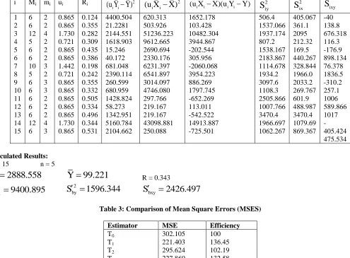
VII. NUMERICAL ILLUSTRATIONS

For numerical illustration of efficiencies of different estimators, we consider data from 1971 census of India, described below. The population consists of 104 blocks (ssu) divided in to N = 15 wards (fsu) of Berhampur City of Odisha. The number of block (Mi)

in 15 wards are 6, 6, 12, 5, 6, 6, 10, 5, 6, 6, 6, 6, 6, 12, 6. The two variables i.e. number of educated females, female pop ulation are used as y, x, respectively. For comparison of Mean square error (MSE) of T0, T1, T2, T3, T4, T5 , we consider 30% sampling fraction at

both the stages. Let the first stage sample size be n= 5 and the sizes of the second stage sample i.e. mi (i = 1, 2, …, 15) are assumed to

(6)

[image:6.612.64.553.79.291.2]

Table 2: Statistical Computations

i Mi mi ui Ri 2

i i

(u Y Y)



(u X

_i _i



X)

2

(u X

i i



X)(u Y

i i



Y)

2 iy

S

2

ix

S

ixy

1 2 3 4 5 6 7 8 9 10 11 12 13 14 15

6 6 12 5 6 6 10 5 6 6 6 6 6 12 6

2 2 4 2 2 2 3 2 3 3 2 2 2 4 3

0.865 0.865 1.730 0.721 0.865 0.865 1.442 0.721 0.865 0.865 0.865 0.865 0.865 1.730 0.865

0.124 0.355 0.282 0.309 0.435 0.386 0.198 0.242 0.355 0.332 0.505 0.334 0.496 0.344 0.531

4400.504 21.2281 2144.551 1618.903 15.246 40.172 681.048 2390.114 260.599 680.959 1428.824 58.273 1342.951 5160.784 2104.662

620.313 503.926 51236.223 9612.665 2690.694 2330.176 6231.397 6541.897 3014.097 4746.080 297.766 219.167 219.167 43098.881 250.088

1652.178 103.428 10482.304 3944.867 -202.544 305.956 -2060.068 3954.223 886.269 1797.745 -652.269 113.011 -542.522 14913.887 -725.501

506.4 1537.066 1937.174 807.2 1538.167 2183.867 1114.678 1934.2 3097.6 1108.3 2505.866 1007.766 3470.4 1966.697 1062.267

405.067 361.1 2095 212.32 169.5 440.267 328.844 1966.0 2033.2 269.767 601.9 488.987 3470.4 1079.69 869.367

-40 138.8 676.318 116.3 -176.9 898.134 76.378 1836.5 -310.2 257.1 1006 589.866 1017 -405.424 475.534

Calculated Results:

N = 15 n = 5

X



2888.558

Y



99.221

_{R = 0.343}

2 bx

S

 

9400.895

S

 

by2

1596.344

S

 

bxy

2426.497

Table 3: Comparison of Mean Square Errors (MSES)

Estimator MSE Efficiency

T0

T1

T2

T3

T4

T5

302.105 221.403 295.624 227.860 221.334 295.693

100 136.45 102.19 132.58 136.49 102.17

Remarks : For the given illustration, it is observed that

 

4

 

1

 

3

 

2

 

5

 

0

MSE T



MSE T



MSE T



MSE T



MSE T



MSE T

VIII. CONCLUSION

The ratio estimators considered in a two stage sampling set up have been compared with the usual unbiased estimator without use of auxiliary information, as regards their efficiencies. The numerical illustration shows that T1 and T4 have nearly equal

efficiency and are more efficient than other competitive estimators.

REFERENCES

[1] Murthy, M.N. (1967). Sampling Theory and Methods. Statistical Publishing Society, Calcutta, India.

[2] Panda, P. (1998). Some Strategies in two-stage sampling using auxiliary information. Unpublished Ph.D. dissertation, Utkal University, Odisha, India.

[3] Sukhatme, P.V., and Sukhatme, B. V. (1970) Sampling theory of Surveys with Applications. Ind. Soc. Agri. Stat., New Delhi

AUTHORS

First Author – Sitanshu Shekhar Mishra, MSC,

[image:6.612.51.546.84.449.2]