The Training and Application of RBF Neural Network Based on GWO

2019 International Conference on Computer Science, Communications and Multimedia Engineering (CSCME 2019) ISBN: 978-1-60595-650-3

The Training and Application of RBF Neural Network Based on GWO

Xiao-qing ZHANG

and Zheng-feng MING

1_{School of Mechano-Electronic Engineering, Xidian University, Xi’an 710000, China}

2

School of Physics and Electronic Engineering, Xianyang Normal University, Xianyang 712000, China

*Corresponding author

Keywords: Grey wolf optimizer, Neural network, Approximation, Chaotic synchronization.

Abstract. To optimize the hidden center matrix, Gaussian RMS width vector and the hidden-output weight matrix of RBF neural network, Grey Wolf Optimizer (GWO) and its several variants have been introduced. With the combination of the three parameters as the position vector of the grey wolf in GWO, selecting half of the average squared error as the optimizing object function, the RBF neural network based on GWO is named as RBF-GWO network. In the processing of training the parameters for RBF-GWO, the difference between the actual output of RBF-GWO network and the desired output value is considered as the guide of updating the position vector for the grey wolf, and in each iteration the optimal parameter values are stored in the position vector of Wolf α which will be returned to the RBF-GWO. The parameter training is completed until the end conditions of the iteration are satisfied. To verify the validity of RBF-GWO network, the continuous function approximation experiment and the chaotic synchronization anti-control experiment have been done in turn. Not only it is proved that the proposed RBF-GWO network is effective, but it is also found that the RBF-GWO network based on the WGWO has a relatively strong adaptive capacity in all experiments from the overall view.

Introduction

The Radial Basis Function (RBF) neural network was proposed by J. Moody and C. Darken. It is characterized by a shallow architecture, self-learning, self-organizing, adaptive, and avoiding local minima problem easily, and has been widely applied in all walks of life [1].

For RBF neural network, along with the economical and scientific development, it has become more difficult to set the weight values only depending on earlier experiences for these changing in real-time, non-linear, dynamic and complex problems. Thus, some better methods are needed to improve the adaptive ability of RBF neural network, or to enhance the fault tolerance ability. The least square method was applied to improve the RBF neural network in [2], the machine learning method was adopted to train the parameters of RBF in [3], and in [4] a variable projection method was used to perfect RBF neural network. Particle Swarm Optimization (PSO) and Genetic Algorithm (GA) were also applied to optimize the parameters of RBF network respectively in [5] and [6], and their optimization effects were very well, which provide a good reference for the application of computational intelligence in RBF network training. Grey Wolf Optimizer (GWO) is a newer computational intelligence algorithm proposed in 2014 [7]. The training of RBF neural network based on GWO and several variant algorithms will be studied.

The GWO Algorithm

Wolf β and Wolf δ are thought as the leaders, and their number are usually set as one, while the number of Wolf ω is set to several dozens or hundreds. In each iterative process, the Wolf ω position is changed on one's own initiative following as Eqs.(1)-(7), but the positions of Wolf α, Wolf β and Wolf δ are passively updated only when the Wolf ω solution is better than the one of Wolf α, Wolf β or Wolf δ.The solution of Wolf α is always optimal in each iteration.

alfa  1 alfa

d C X X , (1)

beta 2 beta

d C X X , (2)

delta 3 delta

d C X X , (3)

1 alfa 1 alfa

X X A d , (4)

2 beta 2 beta

X X A d , (5)

3 delta 3 delta

X X A d , (6)

1 2 3

( 1)

3 t  X X X

X . (7)

where X_alfa, X_beta, and X_delta are the position vectors of Wolf α, Wolf β and Wolf δ respectively,

X is the position vector of Wolf ω in the current iteration, ( 1)X t the position vector in the next

iteration, and ParametersAand C are calculated as following:

1 2   

A a r a (8)

2

2

 

C r (9)

where r1 and r2 are random vectors in [0,1], and Parameter ais a vector that decreases from 2 to 0

with the number of iterations increasing.

When the position value is out of the range, the following calculation could be done as:

max max

min min

, ( ) .

( )

, ( ) .

=

j

j i

i j

i

x if x t x

x t

x if x t x

 

 _

 _. (10)

wherex t_ij( ) is the jth position value of the ith Wolf ω in the current iteration, x_max is the maximum

position value and x_min is the minimum one.

The stochastic search strategy has been adopted in GWO. Because of the characteristics of fast convergence rate, simple structure and easy programming, the GWO has been widely applied [8].

The exploiting ability and exploring ability of GWO are only balanced by a coefficient, and with the number of iterations increasing, its exploiting ability is increased but the exploring ability is greatly weakened, thus it would reduce the optimization speed, and easily fall into the local optimum. Several improved GWO algorithms have been proposed, such as binary GWO (bGWO1 and bGWO2) [9], the improved GWO based on evolutionary population dynamics (GWO-EPD) [10], the optimized GWO based on Mutation Operator and Eliminating-Reconstructing Mechanism (MR-GWO) [11], the modified GWO with hierarchical operators (WWGWO)[12], and the other improved GWO (WGWO) [13] .

RBF Network Based on GWO

To RBF neural network, it is important and difficult to determine the three vectors: the hidden center

vector Φ whose dimension is Nr*Nh, Gaussian RMS width vector Θ whose dimension is Nh*1 and

the hidden-output weight vector ρ whose dimension is Nh*Nn. The “Nn” is the number of the output

neuron. To get three optimized vectors, the GWO is applied in RBF network, and the network is noted as RBF-GWO. In RBF-GWO, the three vectors combination is treated as the position vector of the grey wolf. The optimal objective function is selected as:

2 2

,expec t ,actua l 1

1 2

n

i i i

Object

n 





where n is the number of the samples, yi,expect is the ith expected output,

expect= 1,expect ,expect

T n

y y

 

 

Y and y_i,actual is the ith actual output, Y_actual=_y_1,actual y_n,actual_T.

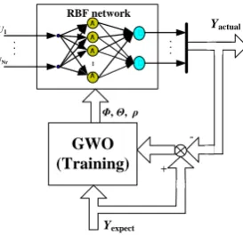
The structure of RBF-GWO is shown in Figure 1. In RBF-GWO, first the samples are sent to the

input ends (U₁,..,U_Nr) for training, the output vector Y_actual is got from the output layer of the RBF

network. After comparing Yactual with the expected output value Yexpect, the compared results will be

transferred to the GWO algorithm, in which the position of the grey wolf may be updated based on the compared results, and finally the Wolf α position vector will be sent back to the RBF network as its

vector parameter Φ, Θand ρ, then one training is completed. One training ending, the next training

starts until the training end condition is satisfied. Simple to understand, the training process of RBF network can be thought as the process to seek the minimum value of Eq. (11), and the training problem of RBF-GWO could be thought as a Minimization Problem.

⅀

U1

UNr

Yactual

GWO (Training)

Φ, Θ, ρ

⅀ RBF network

-+

Yexpect

Figure 1. The structure of RBF-GWO.

Although only the structure of RBF network based on the standard GWO has been introduced, the structures of RBF networks based on other GWO variants are similar to the one. Therefore, the other RBF-GWO structures will not need be explained in detail.

Continuous Function Approximation Experiment

To verify the effectiveness of RBF-GWO, three approximate experiments have been done. Three continuous functions are described in Table 1.

Table 1. The description of the three continuous functions.

Function Name Sigmoid Sine Cosine

The range of training sample [-3:0.1:3] [-2pi:0.1:2pi] [1.25:0.05:2.75]

The number of training sample 61 126 31

The range of testing sample [-3:0.05:3] [-2pi:0.05:2pi

]

[1.25:0.04:2.75]

The number of testing sample 121 252 38

The network structure of RBF 1-20-1 1-15-1 1-15-1

The range of vector parameters in GWO [-10,10] [-10,10] [-3,3]

Functional expression y1/ (1 exp(+ x)) ysin(2 )x 7

(cos( / 2))

The approximate results have been shown in Table 2, where AVE is the average error of ten repeated experiments between the output of RBF-GWO network and the expectations of the testing sample, STD is the average standard deviation of ten repeated experiments, and P is the average p value of Wilcoxon Test matching the network approximation output vector with the expected vector of the testing sample when the significance level was 0.05. The P value is more closing to 1, the difference between the network approximation sample and the testing sample is less obvious. In Table 2, the P value in Cosine experiment is bigger than that in Sine experiment, but smaller than that in Sigmoid experiment, meaning the approaching effect in Sigmoid experiment is the best, that in Cosine experiment is the next-best, and it is the most difficult to approximate the Sine function. Moreover, in the Sigmoid experiment, whether measured from P or AVE value, the approximation effect of RBF-GWO networks based on WGWO, GWO-EPD, MR-GWO and WWGWO are very well. In the Cosine experiment, the networks with P value above 0.9 included WGWO, GWO-EPD, MR-GWO and WWGWO, and the P value based on GWO was about 0.9. According to the results of Sine experiment, the P values based on WGWO, GWO and MR-GWO were greater than 0.8.

Table 2. The approximate results of RBF-GWO.

Algorithm WGWO GWO bGWO1 bGWO2 GA GWO-EPD MR-GWO WWGWO

Sigmoid

AVE 0.0008 0.001

0

0.2490 0.3202 0.015

9

0.0012 0.0011 0.0009

STD 0.0005 0.000

9

0.8720 0.8163 0.012

4

0.0009 0.0008 0.0006

P 0.9893 0.991

6

0.4222 0.3306 0.747

5

0.9854 0.9947 0.9858

Cosine

AVE 0.0152 0.011

2

0.0540 0.0525 0.036

2

0.0119 0.0105 0.0183

STD 0.0141 0.008

9

0.0629 0.0408 0.025

7

0.0101 0.0078 0.0221

p 0.9285 0.891

2

0.5225 0.5989 0.727

2

0.9330 0.9152 0.9620

Sine

AVE 0.1033 0.117

5

0.1085 0.0832 0.051

4

0.1432 0.0550 0.1440

STD 0.4131 0.427

6

0.2987 0.2429 0.074

4

0.4263 0.1579 0.4887

p 0.8644 0.827

6

0.5413 0.6216 0.692

4

0.7717 0.8838 0.6790

To consider all algorithms more clearly, the total mean results are obtained as Table 3. The MAVE is the overall mean error of the three approximate experiments, the MSTD is the overall average standard deviation, and the M-p is the overall average p value for the RBF-GWO network based on each algorithm. From the results, it is obvious that the RBF-GWO network based on MR-GWO, WGWO and GWO is better than others when the approximation effect was measured by MAVE and M-p, and this result is in good agreement with the results in table 2. Generally, RBF-GWO networks can approach the continuous functions very well, especially based on WGWO and MR-GWO.

Table 3. The overall results of approximate experiments.

Algorithm MAVE MSTD M-rate

WGWO 0.03979

4

0.14257 7

0.92736 5

GWO 0.04323

4

0.14579 9

0.90348 6

bGWO1 0.13714 0.4112 0.49532

1

bGWO2 0.15197

7

0.36666 9

0.51704 8

GA 0.03447

6

0.03749 7

0.72235 9

GWO-EPD 0.05206

8

0.14575 8

0.89671 2

MR-GWO 0.02220

4

0.05552 5

0.93125 7

WWGWO 0.05436 0.17046

2

0.87556 6

The Application of RBF-GWO in Chaotic Synchronization

Since 1975 chaos has became a hot topic in the kinetic theory field, especially in nonlinear systems. Although chaos has many definitions, no matter which definition, chaos have the same characteristics: the sensitivity to initial conditions, the aperiodic, fractal dimension and so on.

In this experiment, the PMSM chaotic systems are involved, as Eq. (12) and Eq. (13). The system of Eq. (12) will be as the reference model, and the one of Eq. (13) will be as the controlled system which will be controlled by RBF-GWO to make it synchronized with the system of Eq. (12).

1 1 2 3

2 2 1 3 3

3 2 1

17.5

5.46( )

m m m m d

m m m m m q

m m m L

y y y y v

y y y y y v

y y y T

 _{   }

 _{    }

 

  



(12)

1 1 2 3

2 2 1 3 3

3 2 1

28

3( )

d

q

L

y y y y v

y y y y y v

y y y T

      _{    } 

 _{  } 

(13)

where y₁ and y_m1are the normalized state variables of direct axis current, y₂ and y_m2 are the

normalized state variables of quadrature axis current, y₃ andy_m3are the normalized state variables of

angular velocity, the vd and vq are the normalized variables of direct axis voltage and quadrature

axis voltage respectively, and the T_L is the load torque.

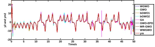
Here, it is assigned that v_d 0, v_q 0and T_L 0, and the synchronization results have been

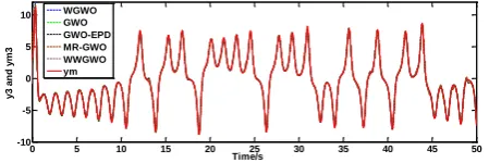
shown in Figs. 2-7. Figure 2, Figure 4 and Figure 6 are the results under controlling of RBF-GWO based on all algorithms including WGWO, GWO, bGWO1, bGWO2, GA, GWO-EPD, MR-GWO, and WWGWO. What can be seen obviously is that the results about bGWO1, bGWO2, and GA are not as good as others, since there are more failing tracking points than others. Therefore, Figure 3, Figure 5, and Figure 7 have been given without the algorithms of bGWO1, bGWO2, and GA. And in

Figure 3, Figure 5, and Figure 7, it is shown obviously that they₁, y₂, andy₃can effectively track

they_m1, y_m2, andy_m3 respectively. To more clearly show the synchronization effect, 5001 points have

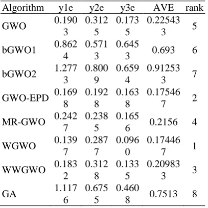
been sampled with 0.01s for time interval in the range of [0, 50s]. The chaotic synchronization

controlling errors of RBF-GWO based on all algorithms are shown in Table 4, where y e1 is the

average value of e₁ y_m1y₁, 2y eis the average value of e₂  y_m2y₂, 3y eis the average error of

3 m3 3

e y y , and the AVE is the total average output errors about Y_mY. From the AVE, the

RBF-GWO network based on WGWO shows the best synchronous controlling effect, the one based on GWO-EPD takes the second place, and the one based on WWGWO takes the third place.

0 5 10 15 20 25 30 35 40 45 50

0 5 10 15 20 25 30 35

Time/s

y

1

a

n

d

y

m

WGWO GWO GWO-EPD MR-GWO WWGWO ym

Figure 2. They₁homogeneous synchronous results of all algorithms.

0 5 10 15 20 25 30 35 40 45 50

-20 -10 0 10 20

Time/s

y

2

a

n

d

y

m

2

WGWO GWO bGWO1 bGWO2 GA GWO-EPD MR-GWO WWGWO ym

0 5 10 15 20 25 30 35 40 45 50 0

10 20 30

Time/s

y

1

a

n

d

y

m

1

WGWO

GWO bGWO1 bGWO2

GA GWO-EPD MR-GWO WWGWO

ym

Figure 4. They₂homogeneous synchronous results of all algorithms.

0 5 10 15 20 25 30 35 40 45 50

-10 -5 0 5 10 15 20

Time/s

y

2

a

n

d

y

m

2

WGWO GWO GWO-EPD MR-GWO WWGWO ym

Figure 5. They₂homogeneous synchronous results without the ones of bGWO1, bGWO2, and GA.

0 5 10 15 20 25 30 35 40 45 50

-5 0 5 10

Time/s

y

3

a

n

d

y

m

3

WGWO GWO bGWO1 bGWO2 GA GWO-EPD MR-GWO WWGWO ym

Figure 6. They₃homogeneous synchronous results of all algorithms.

0 5 10 15 20 25 30 35 40 45 50

-10 -5 0 5 10

Time/s

y

3

a

n

d

y

m

3

WGWO GWO GWO-EPD MR-GWO WWGWO ym

Figure 7. They₃homogeneous synchronous results without the ones of bGWO1, bGWO2, and GA.

Summary and Discussion

Table 4. The errors of the homogeneous synchronous.

Algorithm y1e y2e y3e AVE rank

GWO 0.190

3

0.312 5

0.173 5

0.22543

3 5

bGWO1 0.862

4

0.571 3

0.645

3 0.693 6

bGWO2 1.277

3

0.800 9

0.659 4

0.91253

3 7

GWO-EPD 0.169

8

0.192 8

0.163 8

0.17546

7 2

MR-GWO 0.242

7

0.238 5

0.165

6 0.2156 4

WGWO 0.139

7

0.287 7

0.096 0

0.17446

7 1

WWGWO 0.183

2

0.312 8

0.133 5

0.20983

3 3

GA 1.117

6

0.675 5

0.460

8 0.7513 8

Acknowledgement

This research was supported by the Education and Teaching Reform Research Project of Xianyang Normal University (NO.2017Y004), and partly supported by the Local Service Researching project of Xian Yang Normal University (NO.XSYK18048).

References

[1] Q. Zhou, P. Shi, S. Xu, et al, Observer-based adaptive neural network control for nonlinear stochastic systems with time delay. IEEE Trans. Neural Netw. Learn. Syst. 24 (2013) 71-80.

[2] F. Ding, P.X. Liu, G. Liu, Multi-innovation least-squares identification for system modeling. IEEE Trans. Syst. Man, Cybern. B, Cybern. 40 (2010) 767-778.

[3] G.B. Huang, H. Zhou, X. Ding, R. Zhang, Extreme learning machine for regression and multiclass classification. IEEE Trans. Syst. Man, Cybern. B, Cybern., 42 (2012) 513-529.

[4] M. Gan, H.X. Li, H. Peng, A variable projection approach for efficient estimation of RBF-ARX model. IEEE T. Cybernetics 45 (2015) 476-485.

[5] V. Fathi, G.A. Montazer, An improvement in RBF learning algorithm based on PSO for real time applications. Neurocomputing 111 (2013) 169–176.

[6] D.W. Chen Research on traffic flow prediction in the big data environment based on the improved RBF neural network. IEEE T. Ind. Inform. 13 (2017) online.

[7] S. Mirjalili, S.M. Mirjalili, A. Lewis, Grey wolf optimizer. Adv. Eng. Softw. 69 (2014) 46-61.

[8] X.Q. Zhang, Z.F. Ming, Trajectory Planning and Optimization for a Par4 Parallel Robot Based on Energy Consumption. Appl. Sci-basel. 9 (2019) 2770.

[9] E. Emary, H.M. Zawbaa, A.E. Hassanien, Binary grey wolf optimization approaches for feature selection. Neurocomputing 172 (2016) 371-381.

[10] S. Saremi, S.Z. Mirjalili, S.M. Mirjalili, Evolutionary population dynamics and grey wolf optimizer, Neural. Comput. Applic. 26 (2015) 1257-1263.

[12] L. Rodríguez, O. Castillo, J. Soria, et al. A fuzzy hierarchical operator in the grey wolf optimizer algorithm. Appl. soft comput. 57 (2017) 315-328.