Perfect Simulation from Non-neutral Population
Genetic Models: Variable Population Size and
Population sub-division
Paul Fearnhead1
1. Department of Mathematics and Statistics, Lancaster University, Lancaster, LA1 4YF, UK
Summary: We show how the idea of monotone coupling from the past can produce sim-ple algorithms for simulating samsim-ples at a non-neutral locus under a range of demographic models. We specifically consider a biallelic locus, and either a general variable population size mode, or a general migration model for population subdivision. We investigate the effect of demography on the efficacy of selection, and the effect of selection on genetic divergence between populations.
Keywords: Ancestral Selection Graph, Coupling from the Past, Demes, Frequency
1
Introduction
While simulating from neutral population genetics models is straightforward using the coalescent (Kingman, 1982), even for complex demographic models (see e.g. Donnelly and Tavar´e, 1995; Hudson, 2002), simulation from non-neutral models is much more difficult. There are currently numerous approaches to simulation for non-neutral models. These can be split into two cases, simulating from the stationary distribution of the population, or simulating from the population at a specfic time. Examples of the latter include simulating samples a specific time after the fixation of a beneficial allele (e.g. Przeworski, 2003). In this paper we focus on the former.
For non-neutral models which assume parent-independent mutation, constant population size and random-mating, the stationary distribution of allele frequencies is known and can be simulated from directly using rejection sampling (Donnelly et al., 2001) or numerical integration methods (Fearnhead and Meligkotsidou, 2004; Joyce and Genz, 2006). For such models it is also possible to simulate the genealogy of a sample, and linked neutral variation. This is possible by simulating and conditioning on the frequency of the non-neutral allele in the history of the population(Spencer and Coop, 2004; Coop and Griffiths, 2004; Nordborg, 2001; Nordborg and Innan, 2003), or by simulating from the conditional distribution of the ancestral selection graph given the allelic type of the sample (Slade, 2000; Stephens and Donnelly, 2003; Fearnhead, 2006)
For models which do not assume parent-independent mutations, it is possible to use coupling-from-the-past (CFTP) (Propp and Wilson, 1996; Kendall, 2005) to simulate sam-ples from the ancestral selection graph (Fearnhead, 2001). Here we extend this idea. Firstly we introduce a simpler implementation of CFTP, which is obtained by having a state-space of unordered rather than ordered samples. This means that we characterise a sample by the number of alleles of each type, rather than by the allelic type of each of an ordered set of chromosomes. This has two advantages, firstly that as we work on a smaller dimensional space, coupling should be quicker. Secondly, for the models we consider, by working with unordered samples we obtain a monotonicity of the sample space, which makes it more straightforwad to detect when we have obtained a sample from the stationary distribution of interest, and thus provides a much simpler algorithm to implement.
from such multiple deme coalescent models in the presence of selection. Our method is computationally efficient, with for example 1,000 samples of size 100 being simulated in less than 40s for a 10 deme stepping-stone model under a variety of selection models (see RESULTS).
2
Methods
Monotone Coupling From The Past
Consider an ergodic Markov chain Xt with state space {0,1, . . . , K}. Coupling from the
past (CFTP; Propp and Wilson, 1996) gives a method for simulating from the stationary distribution of Xt. The idea is based on the fact that if we simulated the Markov chain
from time −∞ to time 0, then regardless of the initial value of the chain, X−∞, we would have that X0 is a draw from the stationary distribution of the chain. The idea of CFTP is that it enables us to perform such simulation in finite computing time.
To do this we first introduce some extra simulation, in that we consider simulating the value of Xt+1 for all possible values of Xt. To simplify notation we will define a function Ft(·)
which specifies all these transitions. So if we are told that Xt =x, then we have Xt+1 =
Ft(x). Note that the functionFt is a realisation of a random variable; the stochasticity of
the Markov chain is now encompassed in the randomness of this function, but given a set of realisations F−T, F−T+1, . . . , F−1 we have a deterministic relationship betweenX−T and
X0.
We now have an idealised simulation algorithm:
(a) Fort =−1,−2, . . . ,−∞ simulate the value ofXt+1 for all possible values of Xt; and
hence the function Ft(·).
(b) Arbitrarily specify X−∞; and for t=−∞, . . . ,−1 recursively apply xt+1 =Ft(xt) to
obtain x0, a draw from the stationary distribution of the Markov chain.
This algorithm is obviously impracticable, as it involves infinite computing time. However we can perform this simulation in finite computing time by doing this simulation a bit at a time. This gives the following CFTP algorithm:
(a) Arbitrarily choose a negative integer T0; set T =T0 and S = 0.
(c) For each possible starting value x = 0,1, . . . , K, set XT = x and recursively apply
xt+1 = Ft(xt) to obtain x0. If the value of x0 is identical for all starting values of
Xt then output x0, a draw from the stationary distribution of the Markov Chain;
otherwise set S =T, T = 2T and return to (b).
The idea here is that we imagine that we are doing the idealised simulation algorithm above. However, we first simulate the dynamics of the chain from time T0 to time 0; then the extra dynamics from time 2T0 to time T0; then the extra dynamics from time 4T0 to times 2T0 and so on (step b). The coupling condition in step (c) enables us to determine with certainty what the value ofX0 would be if we had continue to simulated the dynamics of the chain back to time −∞ (as in the idealised algorithm). For example, imagine that the condition in step (c) is satisfied after simulating back to time 4T0; this condition says that regardless of the value of X4T0, the value of X0 will be the same (x0). Thus we do not
need to know the realisation of the chain from time −∞ to time 4T0, as regardless of this we know that continuing the realisation on to time 0 will produceX0 =x0. Thus the value we output in step (c) is the same as the value we would obtain in step (b) of the idealised simulation algorithm, and is thus a draw from the stationary distribution of the Markov chain.
Any choice for how to decrease T when coupling does not occur would produce a valid algorithm, but it has been argued that doublingT each time is optimum (by its relationship with a binary search; see e.g. Kendall, 2005). Note that the validity of the approach requires that we do not resimulate any of the dynamics of the Markov chain if coupling does not occur in step (c). Furthermore, the algorithm requires only that the functions Ft(·) are
simulated in such a way that marginally the dynamics of the Markov chain are correct, and it is possible to have any amount of dependence in terms of the value of Xt+1 for different values of Xt. In some cases it is possible to utilise this to obtain a more efficient way
of determining whether coupling occurs in step (c). If we can find a distribution on Ft,
which marginally has the dynamics of the Markov chain, and that staisfies the monotonicty condition that x≥y⇒F(x)≥F(y) then we can replace step (c) with:
(c) For bothx= 0 andx=K, setXT =xand recursively applyxt+1=Ft(xt) to obtain
x0. If the value ofx0 is identical for both starting values ofXtthen outputx0, a draw
from the stationary distribution of the Markov Chain; otherwise set S =T,T = 2T
the Markov chain forward in time for the minimal and maximal elements of the state-space. The monotonicity ensures that if these two realisations couple, then all realisations from other starting points (which lie between them) will also couple.
While in this example we have assumed a totally ordered state-space, monotone CFTP will still apply if we have only a partial order: if starting the chain at each of the maximal and minimal elements of our state-space produce the same x0 value, then so must all other starting values of the chain (which lie between the minimal and maximal elements). We will use this extension to partial orderings in the multi-deme models we consider below. An example of the CFTP algorithms is given in Figure 1.
Models
We consider coalescent models which include selection, variable population size and pop-ulation structure, and focus on a single biallelic locus. Details of how selection is incor-porated within a coalescent-type process can be found in work on the Ancestral Selection Graph (Krone and Neuhauser, 1997; Neuhauser and Krone, 1997) or the Ancestral In-fluence Graph (Donnelly and Kurtz, 1999). For background on incorporating population growth or population structure see for example Donnelly and Tavar´e (1995) and Hudson (1990) and references therein.
The coalescent model we consider is obtained in the large population size limit to a range of forward population genetics model. We briefly describe how the parameters are defined in the case of the Wright-Fisher model. Firstly define an effective population size of N0 diploid individuals, or equivalently 2N0 chromosomes. We measure time in units of 2N0 generations, and as is common define time in terms of time before the present. We consider a population consisting of D demes, with random mating within each deme. At time t in the past, the population size of deme d is Nd(t) = N0λd(t) diploid individuals. For the
case D >1 we further define a migration matrix by Mij = 4N0mij for i6=j, wheremij is
the proportion of the population of deme i in a generation that have migrated there from deme j in the previous generation. We define Mi =
P
j6=iMij.
We denote the alleles at our locus by 1 and 2. As with any biallelic model, mathematically we can describe the mutation process in terms of parent-independent mutations. We let
θ = 4N0u, whereu is the probability of mutation per chromosome per generation, and let
ν = (ν1, ν2) be the probability distribution of the mutant allele. (Note that this model allows for “silent” mutations, which do not change the allele at the locus; thus the effective mutation rate of allele 2 to allele 1 is θν1, and of allele 1 to allele 2 is θν2.)
4
3
2
1
0
STATE
0
−8 −7 −6 −5 −4 −3 −2 −1
[image:7.595.117.483.195.413.2]Time
1 +sij for i, j = 1,2, with sij ≥ 0 and s12 =s21, We can thus define selection rates σij∗ =
4N0sij. We choose a different parameterisation of these selection rates where σ11∗ = σ11,
σ∗
12 = σg +σ12 and σ22∗ = 2σg +σ22. This is an over-parameterisation of the selection
process, and any choice of σg ≥0 and σij ≥0 fori, j = 1,2 which gives the correct values
of σ∗
ij could be used. We then define σ= max{σ11, σ12, σ22}.
The choices of defining the mutation process in terms of a parent-independent mutation process, and the parameterisation of selection rates, have been made in order to make the simulation algorithm detailed below as efficient as possible. In particular the parameteri-sation of the selection rates is in terms of a genic component (given by the σg terms) and
a non-genic component. The efficiency of the simulation algorithm is increased by choos-ing σg to be as large as possible subject to the constraints on the positivity of the other
selection rates. (To do this we should label the alleles so that σ∗
22 ≥σ∗11.)
For ease of presentation we have assumed that the selection rates are constant through time and across demes; though it is straightforward to generalise to the case where these rates vary. The coalsescent process for our above model can be described in terms of a backward process for the history of our sample (which is independent of the alleles in the sample) and conditional on this backward process some forward dynamics for the allelic types of the branches. If we simulated the backward process until timet =∞, then for any initial choice for the population frequency of the alleles at that time, when we simulated the process forward we would obtain a sample at the present time which is drawn from the stationary distribution of the population. We now describe these backward and forward processes and how we can appply monotone CFTP.
Backward Process
The Backward Process is a continuous time Markov Chain, whose stateN(t) = (N1(t), . . . ,ND(t)) is the number of branches in the underlying coalscent-type process at time t in the past
that come from each deme. The transitions correspond to different possible events in this coalescent-type process. To ease notation, let the state at current timetbe (n1, n2, . . . , nD),
then the rates of the possible events, and the corresponding transitions, are:
(i) Coalescence, demedoccurs at ratend(nd−1)/(2λd(t)); with transitionnd =nd−1.
(ii) Migration, deme d to deme ioccurs at rate ndMdi/2;with transition nd=nd−1
and ni =ni+ 1.
(iv) Genic Selection, deme d occurs at rate ndσg/2; with transitionnd=nd+ 1.
(v) Diploid Selection, deme d occurs at rate ndσ/2; with transition nd=nd+ 2.
(When describing the transition we have listed only the elements of the state that change.) The initial value of the state, N(0) is given by the number of chromosomes sampled from each deme.
Forward Dynamics and Monotone CFTP
Assume we have simulated and stored T events in the backward process above. We now consider the forward in time dynamics; however in order to apply CFTP we need to make these forward dynamics deterministic, and thus for each event that we simulate in the backward process we also simulate and store a realisation of an independent continuous uniform [0,1] random variable. These realisations will then determine the specific forward transition at each event.
Forward in time the state of our system is given by the number of each type of allele in each deme in our ancestral process. As we have stored the number of branches in each deme at each event, we can define this state solely in terms of the number of type 1 alleles in each deme; which we denote by n(1) = (n(1)1 , . . . , n(1)D ). Our forward in time dynamics are determined by specifing an initial value for the state n(1). Then for the Tth event,
T −1th event, . . . , 1st event in turn we update this state as follows.
Consider the jth event. Let u denote the realisation of the uniform random variable associated with this event. Assume the current state is n(1), and the number of branches in each deme isn = (n1, . . . , nD). Then the dynamics depend on the type of the jth event
as follows:
(i) Coalescence, deme d; ifu < n(1)d /nd then let n
(1)
d =n
(1)
d + 1.
(ii) Migration, deme d to deme i; if u < n(1)i /ni then let n(1)d =n(1)d + 1 and n(1)i =
n(1)i −1.
(iii) Mutation demed; ifu <(nd−n(1)d )ν1/ndthen letn(1)d =n(1)d +1; ifu >1−n(1)d ν2/nd
then let n(1)d =n(1)d −1.
(iv) Genic Selection, deme d; if u < 1−(nd−n(1)d )(nd−n(1)d −1)/(nd(nd−1)) then
(v) Diploid Selection, deme d; if
u < n
(1)
d (n
(1)
d −1)(n
(1)
d −2 + (σ−σ11+σ12)(nd−n
(1)
d )/σ)
nd(nd−1)(nd−2)
, (1)
then let n(1)d =n(1)d −2; otherwise if
u <1− (nd−n
(1)
d )(nd−n
(1)
d −1)(nd−n
(1)
d −2 + (σ−σ22+σ12)n
(1)
d /σ)
nd(nd−1)(nd−2)
, (2)
then let n(1)d =n(1)d −1.
We have described the dynamics purely in terms of changes in n(1), the changes in the number of branches in each deme is given by the reverse of the dynamics of the backward process. These dynamics come from the different possible events in the coalescent process that would affect n(1). For (i) this is a coalescent event to branch of allele 1; for (ii) a migration of an allele 1 branch from population i to d; for (iii) a mutation of an allele 2 branch to allele 1, or vice-versa; for (iv) a selection event at which an allele 1 branch is non-ancestral (which occurs unless both incoming and continuing branches have allele 2); and for (v) a selection event at which both non-ancestral branches have allele 1, or only one has. (See Appendix A for the calculation of the probabilities in this case).
We can now use CFTP to simulate a sample from the stationary distribution of the pop-ulation. The dynamics specified above satisfy a monotonicity condition (see Appendix B) if 2σ21 ≤ σ + σ11 + σ22. (This can always be achieved by, if necessary, choosing
σ > max{σ11, σ12, σ22}; for example if σ11 = σ22 = 0 as in heterozygote advantage then we choose σ = 2σ12.) The partial ordering of this monotonicity is that (n1, . . . , nD) ≥
(n′
1, . . . , n′D) if and only if nd≥n′d for d= 1. . . , D.
Thus the monotone CFTP algorithm described above can be applied, whereby to check coupling we need only run the process forward in time from two values of the state: n(1) = (n1, . . . , nD), all branches in all demes carry allele 1, and n(1) = (0, . . . ,0), no branches in
any deme carry allele 1. If we obtain the same sample from each of these initial conditions, then that sample is drawn from the population at stationarity. If not we have to simulate the backward process further into the past and repeat until coupling occurs.
Programs implementing CFTP for both single-population variable population size and for multiple-deme constant-population size models were written in a combination of R and C. These are available from www.maths.ac.uk/∼fearnhea.
To check the validity of the programs implementing this monotone CFTP algorithm we ran the programs under two special cases. Firstly we considered the neutral case, and compared the results of our program with those obtained by the program ms (Hudson,
2002). Note that this program defines time in units of N0 generations, rather than the 2N0 used here. It assumes an infinite sites mutation model - this output can be converted into a 2-allele model with ν = (0.5,0.5) by (i) setting the mutation rate it θ/2, and (ii) assuming each mutation changes the allele of the chromosome so that the allele of a chromosome is determined by whether it has an odd or an even number of mutations. For the constant population size and a single panmictic population (D= 1) we compared results with those based on simulating from the known stationary distribution of the population frequency of allele 1 using rejection sampling (see Donnelly et al., 2001).
3
Results
Single-Population Model
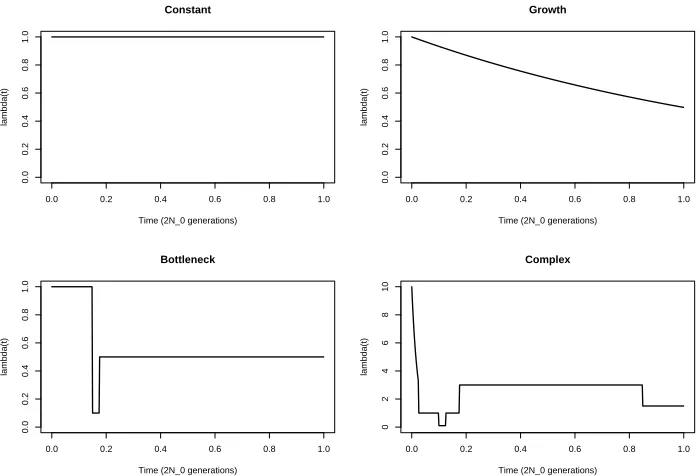
First we used the CFTP algorithm to simulated from a series of single population models. There are many demographic models that have been suggested or inferred for human or other populations (e.g. Wakeley et al., 2001; Wallet al., 2002; Marthet al., 2004; Schaffner et al., 2005). We considered four different scenarios for the variation in population size, and four different selection models. In each case we set N0 = 10,000 diploid individuals,
θ = 1 and ν = (0.9,0.1) (based loosely on appropriate mutation models for disease genes; see Pritchard, 2001). The four population size scenarios are:
Constant A constant population size.
Growth An exponentially growing population with λ(t) = exp(−0.7t) (based on an
in-ferred model for beta-globin, see Harding et al., 1997).
Bottleneck A population bottleneck from t = 0.15 to t = 0.175. During the bottleneck
the effective population size is 1,000, and prior to it it is 5,000. (based on a model from Marth et al., 2004).
Complex A more complicated scenario based loosely on the population-size of a
0.0 0.2 0.4 0.6 0.8 1.0 0.0 0.2 0.4 0.6 0.8 1.0 Constant
Time (2N_0 generations)
lambda(t)
0.0 0.2 0.4 0.6 0.8 1.0
0.0 0.2 0.4 0.6 0.8 1.0 Growth
Time (2N_0 generations)
lambda(t)
0.0 0.2 0.4 0.6 0.8 1.0
0.0 0.2 0.4 0.6 0.8 1.0 Bottleneck
Time (2N_0 generations)
lambda(t)
0.0 0.2 0.4 0.6 0.8 1.0
0 2 4 6 8 10 Complex
Time (2N_0 generations)
[image:12.595.120.470.135.373.2]lambda(t)
Figure 2: Plots of λ(t) = N(t)N0 for the four population-size scenarios.(Note the diffent scale for the Complex scenario.)
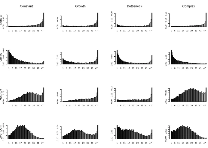
Plots of λ(t) =N(t)/N0 for each of these models are given in Figure 2 The selection models are defined in terms of the selection ratesσ∗ = (σ∗
11, σ∗12, σ22∗ ). Our four selection models are (i) Neutral σ∗ = (0,0,0); (ii) Genic σ∗ = (0,5,10); (iii) Heterozygote advantage σ∗ = (0,10,0); and (iv) Heterozygote overdominance σ∗ = (0,20,10). For each combination of population size scenario and selection model we simulated 10,000 samples. The CPU cost varied across the 16 pairs we considered. In the constant population-size case, on a 3.4GHz Laptop, it took 0.3s, 1s, 15s and 25s to simulate 1,000 samples for the four selection models respectively. CPU times were reduced by around a factor of 2 for the Growth and Bottleneck scenarios, and were increased by around a factor of 1.5 for the Complex scenario.
1 6 11 17 23 29 35 41 47
0.00
0.10
Constant
Neutral
1 6 11 17 23 29 35 41 47
0.00
0.10
Growth
1 6 11 17 23 29 35 41 47
0.00
0.10
0.20
Bottleneck
1 6 11 17 23 29 35 41 47
0.00
0.10
0.20
Complex
1 6 11 17 23 29 35 41 47
0.00
0.04
0.08
Genic
1 6 11 17 23 29 35 41 47
0.00
0.06
1 6 11 17 23 29 35 41 47
0.00
0.06
1 6 11 17 23 29 35 41 47
0.00
0.06
1 6 11 17 23 29 35 41 47
0.00
0.03
Het Adv
1 6 11 17 23 29 35 41 47
0.00
0.06
1 6 11 17 23 29 35 41 47
0.00
0.06
0.12
1 6 11 17 23 29 35 41 47
0.000
0.020
1 6 11 17 23 29 35 41 47
0.00
0.02
0.04
Over Dom
1 6 11 17 23 29 35 41 47
0.00
0.02
0.04
1 6 11 17 23 29 35 41 47
0.00
0.02
1 6 11 17 23 29 35 41 47
0.000
[image:13.595.124.470.261.508.2]0.020
most pronounced for the Heterozygote Advantage case where the Growth and Bottleneck scenarios have substantially reduced any effect of selection.
Two Deme Model
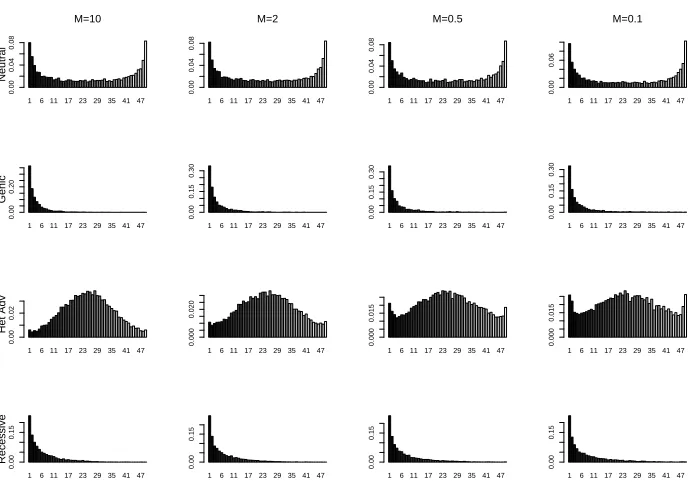
We now consider a model based on two demes each containing a constant-sized panmictic populations with migration between the demes. For simplicity we assume each deme has the same population size, and idential migration rate from deme 1 to deme 2 and vice versa. We assume a total sample of size 100, with 50 chromosomes sampled from each deme. We assume ν = (0.5,0.5) and present results for θ = 0.1. We obtain very similar results for smaller values of θ except that the probability of the allele segregating in the population is reduced.
We present results for four selection models and four migration rates. Again we summarise the selection models in terms of σ∗ = (σ∗
11, σ12∗ , σ∗22). Our four selection models are (i) Neutralσ∗ = (0,0,0); (ii) Genicσ∗ = (0,5,10); (iii) Heterozygote advantageσ∗ = (0,10,0); and (iv) Recessive σ∗ = (0,10,10). The four migration rates (the values of M
12 = M21) are 10, 2, 0.5 and 0.1.
We simulated 10,000 samples for each of the 16 combinations of selection model and migra-tion rate. We verified the results for the neutral model with other simulamigra-tion methods (see Verifying the CFTP Results). The CPU cost of the simulation varied little with migration, and was approximately 0.4s, 0.7s, 10s and 4s per 1,000 samples for the four selection mod-els respectively (CPU times for a 3.4GHz Laptop). The frequency spectrum for samples of size 50 within a single deme, conditional on the allele segregating are shown in Figure 4. The amount of migration appears to have little effect except in the case of heterozygote advantage, when smaller migration rates appear to reduce the effect of selection.
We also studied the effect of selection and the degree of divergence in gene frequency be-tween the demes. Table 1 gives the mean Fst values for samples under a SNP ascertainment model which requires 2 randomly chosen chromosomes (across both demes) to segregate. If the observed frequency of type 1 alleles in the demes were p1 and p2 respectively, and
p= (p1+p2)/2, then the Fst value for that sample was (p1−p)2/(p(1−p)) (see e.g Section 2.3 of Nicholson et al., 2002). The weight given to a sample is proportional to p(1−p), and gives more importance to samples whose minor allele frequency is close to 0.5.
As noted by Hugheset al.(2005), the effect of selection is to reduce the amount of variation in allele frequencies, and hence Fst values, across demes. The effect is most pronounced as migration rates are decreased. (Measuring the variation in allele frequencies using the
1 6 11 17 23 29 35 41 47 0.00 0.04 0.08 M=10 Neutral
1 6 11 17 23 29 35 41 47
0.00
0.04
0.08
M=2
1 6 11 17 23 29 35 41 47
0.00
0.04
0.08
M=0.5
1 6 11 17 23 29 35 41 47
0.00
0.06
M=0.1
1 6 11 17 23 29 35 41 47
0.00
0.20
Genic
1 6 11 17 23 29 35 41 47
0.00
0.15
0.30
1 6 11 17 23 29 35 41 47
0.00
0.15
0.30
1 6 11 17 23 29 35 41 47
0.00
0.15
0.30
1 6 11 17 23 29 35 41 47
0.00
0.02
Het Adv
1 6 11 17 23 29 35 41 47
0.000
0.020
1 6 11 17 23 29 35 41 47
0.000
0.015
1 6 11 17 23 29 35 41 47
0.000
0.015
1 6 11 17 23 29 35 41 47
0.00
0.15
Recessive
1 6 11 17 23 29 35 41 47
0.00
0.15
1 6 11 17 23 29 35 41 47
0.00
0.15
1 6 11 17 23 29 35 41 47
0.00
[image:15.595.124.469.148.394.2]0.15
Figure 4: Histograms of the frequency of allele 1 in a sample of size 50 from a single deme (conditional on the allele segregating) for each pair of migration rate and selection model. See text for full details of the models.
M = 10 M = 5 M = 0.5 M = 0.1 Neutral 0.035 0.123 0.326 0.650
Genic 0.031 0.070 0.127 0.218 Het Adv 0.031 0.080 0.159 0.295 Recessive 0.033 0.083 0.149 0.199
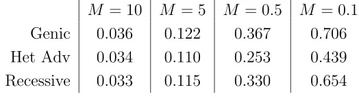
[image:15.595.174.427.524.608.2]M = 10 M = 5 M = 0.5 M = 0.1 Genic 0.036 0.122 0.367 0.706 Het Adv 0.034 0.110 0.253 0.439 Recessive 0.033 0.115 0.330 0.654
Table 2: Mean Fst values (based on 10,000 samples) under a 2-deme model with different selection regimes within each deme. We assumed neutrality within deme 1, and either the genic, heterozygote advantage or recessive selection model for deme 2. Results are given for different migration rates (M). A weighted mean was calculated with the Fst value from each sample being weighted by the probability that 2 randomly chosen chromosomes carry different alleles. See text for full details of the models.
We further tested the effect of different selection regimes within the two demes. For sim-plicity we assumed neutrality within deme 1, and the three selection models above within deme 2. The mean Fst values in this case are given in Table 2. As expected Fst values increased as compared to the case of the same selection regime within each population, though only in the genic selection case are Fst values consistently greater than in the completely neutral case.
Stepping Stone Model
We now consider a linear (circular) stepping stone model . We assume 10 ordered demes, each of equal population size. Migration events are possible between neighbouring demes, with Mi,i+1 = Mi+1,i = 1 for i = 1, . . . ,9 and M1,10 = M10,1 = 1. We consider the same mutation model and each of the four selection models used in the 2 deme case, and simulate samples of size 100, with 50 chromosomes sampled from deme 1, and 50 from deme 1 +c
for c= 1, 2, 3, and 4. We are interested in the degree of correlation in allele frequencies for differing degrees of physical separation of the demes (c) and differing selection models. Again we simulated 10,000 samples for each combination of selection model and c. CPU costs were affected only slightly by c and were 0.5s, 1,4s, 40s and 20s per 1,000 samples for the neutral, genic, heterozygous advantage, and recessive selection models respectively (on a 3.4GHz Laptop). We calculated Fst values in the same way as for the 2 deme case (above), once again under a SNP ascertainment scheme that requires two randomly chosen chromosomes from our sample of size 100 to be carrying different alleles.
c= 1 c= 2 c= 3 c= 4 Neutral 0.19 0.27 0.32 0.34
[image:17.595.198.397.127.217.2]Genic 0.09 0.10 0.10 0.10 Het Adv 0.09 0.11 0.11 0.12 Recessive 0.11 0.12 0.13 0.14
Table 3: Mean Fst values (based on 10,000 samples) under a stepping-stone model for each combination of selection model and spatial separation of the two demes (c). A weighted mean was calculated with the Fst value from each sample being weighted by the probability that 2 randomly chosen chromosomes carry different alleles. See text for full details of the models.
c= 1 c= 2 c= 3 c= 4
σg = 1 0.16 0.22 0.23 0.25
σg = 2 0.13 0.17 0.19 0.17
σg = 3 0.11 0.13 0.14 0.14
σg = 4 0.10 0.11 0.12 0.11
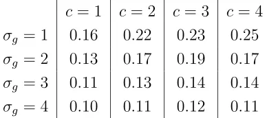
Table 4: Mean Fst values (based on 10,000 samples) under a stepping-stone model for genic selection and different spatial separation of the two demes (c). A weighted mean was calculated with the Fst value from each sample being weighted by the probability that 2 randomly chosen chromosomes carry different alleles. See text for full details of the models.
the amount of variation in allele frequencies depends little on the spatial separation of the demes, which is not the case for the neutral case. We further investigated this effect by simulating samples under the genic model for a range of smaller selection values; σg = 1,
2, 3 and 4 (see Table 4). The effect that Fst values depend little on spatial separation is noticeable for σg ≥2.
4
Discussion
[image:17.595.202.396.330.416.2]problems we consider. Thus simulating samples only requires (i) to simulate the number of branches within the ancestral selection graph back in time; and (ii) to simulate the number of these branches (within each deme) that carry allele 1 forward in time for two initial configurations: all branches initially carrying allele 1 and all branches initially carrying allele 2. The resulting algorithm has been shown to be computationally efficient, and enables simulation of a large number of samples from complex selection and demographic models within practicable CPU time. The main limitation on the simulation algorithm is the mutation rate θ, with the CPU cost appearing to increase proportional 1/θ for small theta. Thus simulation for very small values of the mutation rate can be prohibitive. The monotonicity characteristic of our models occurs because we consider only a single selective locus which carries two different alleles. For more general models, monotonicity will not necesarily apply, but simulating unordered samples as here should still be easier and more efficient than simulating ordered samples as in Fearnhead (2001).
The examples we considered either assumed a single population and variable population size, or constant population size and multiple demes. There are alternative approaches for analysing and simulating under the former class of models: in some cases direct simulation is possible by simulating the ancestral selection graph back in time until there is a constant population size and then simulating the alleles on the branches at that time from the known stationary distribution of the constant population size model. Alternatively there is recent work by Evanset al.(2006) which calculates the frequency spectrum under variable population size models and an infinite sites mutation model, and the method used with
SelSim (Spencer and Coop, 2004) could easily be adapted to this situation.
However, simulating samples from non-neutral models with multiple demes is much more challenging, and we know of no other current coalescent-based simulation methods in this case. Some methods exist for special cases, for example diffusion approximations for the island model in the limit as the number of demes tends to infinity (Cherry and Wakeley, 2003; Cherry, 2003).
Acknowledgements Motivation for this work came from the ICMS workshop on
Math-ematical Population Genetics, March 2006. This research was supported by Engineering and Physical Sciences Research grant number C531558.
Appendix A: Diploid Selection Dynamics
secong the continuing branch and the third the checking branch; (ii) denote by ij the genotype given be the incoming and checking branch; and (iii) with probability σij/σ the
incoming branch is parental, otherwise the continuing branch is.
Firstly consider the probability of the non-ancestral branches at a diploid selection event both carrying allele 1. This corresponds to the first condition on u given by (1). This occurs if either (a) all three branches chosen in (i) carry allele 1, or (b) if two of these branches carry allele 1 and they are non-ancestral. The probability of (a) is n(1)(n(1)− 1)(n(1)−2)/(n(n−1)(n−2)). The probabilitiy of (b) is
3n(1)(n(1)−1)(n−n(1))
n(n−1)(n−2)
µ
σ12 3σ +
σ−σ11 3σ
,
where the first term is the probability of choosing 2 branches carrying allele 1 and one carrying allele 2; the second the term is the probability of the branch carrying allele 2 being the incoming branch and being ancestral; and the final term is the probability of the branch carrying allele 2 being the continuing branch and being ancestral.
Combining these probabilities gives the expression on the right-hand side of (1).
The right-hand side of (2) is one minus the probability of the two non-ancestral branches carrying allele 2, and is calculated in an identical manner. The probability of u satisfying (2) but not (1) is thus the required probability of the precisely one non-ancestral branches carrying allele 1.
Appendix B: Monotonicity
For notational simplicity we will drop the (1) superscipt for the state. Consider two values for the staten andn′ which satisfy n≥n′. To demonstrate monotonicity we need to show that for any possible event and value of u this ordering of the states is preserved.
Monotonicity at coalescence, mutation and genic selection events hold trivially. Assume one of these events occurs to a branch in demed. Eithernd=n′din which case the dynamics
at this event are identical for both states; or nd ≥ n′d+ 1 in which case the ordering is
preserved as the transition changes the nd and n′d values by either 0 or 1.
Monotonicity also follows for migration events. Consider a migration from demei to deme
d. We need only consider ni 6=n′i, as otherwise the dynamics at this event are identical for
both states. However in this case the ordering is preserved in demeiby the same argument as above; and is also preserved in demedasnd≥n′dand the dynamics mean that whenever
n′
d increases by one then so does nd.
check that it is never possible for n′
d to be unchanged at this event at the same time as nd
being decreased by 2. Again for ease of exposition, we slightly change notation and denote the number of branches in deme d byn. For such a transition to occur we would need
u < nd(nd−1)(nd−2 + (σ−σ11+σ12)(n−nd)/σ)
n(n−1)(n−2) , (3)
for the nd to be decreased by 2 (see Equation 1) and
u >1−(n−nd+ 1)(n−nd)(n−nd−1 + (σ−σ22+σ12)(nd−1)/σ)
n(n−1)(n−2) , (4)
forn′
dto be unchanged (using Equation 2 andn′d=nd−1). Now leta = (σ−σ11+σ12)/(3σ) and b= (σ−σ22+σ12)/(3σ). Inequalities (3) and (4) can simultaneously hold for the same
u if and only if
nd(nd−1)(nd−2 + 3a(n−nd))
n(n−1)(n−2) >1−
(n−nd+ 1)(n−nd)(n−nd−1 + 3b(nd−1))
n(n−1)(n−2) .
Thus for monotonicity we need to show that this cannot occur, and thus that for alln and
nd
n(n−1)(n−2)≥nd(nd−1)(nd−2) + 3nd(nd−1)(n−nd)a+
(n−nd+ 1)(n−nd)(n−nd−1) + 3(n−nd+ 1)(n−nd)(nd−1)b
Now consider the right hand side; this can be re-written as
nd(nd−1)(nd−2) + 3nd(nd−1)(n−nd)−3nd(nd−1)(n−nd)(1−a)+
(n−nd)(n−nd−1)(n−nd−2) + 3(n−nd)(n−nd−1) + 3(n−nd)(n−nd−1)(nd) +
3(n−nd)(3nd−n−1)−3(n−nd+ 1)(n−nd)(nd−1)(1−b)
Now the first, second, fourth and sixth terms of this expression sum to n(n−1)(n−2), so we get that the inequality we required simplifies to
0≥ −3nd(nd−1)(n−nd)(1−a) + 3(n−nd)(n−nd−1)+
3(n−nd)(3nd−n−1)−3(n−nd+ 1)(n−nd)(nd−1)(1−b)
= 3(n−nd)((n−nd−1 + 3nd−n−1)−(1−a)nd(nd−1)−(1−b)(n−nd+ 1)(nd−1))
Now this inequality trivially holds for nd = 1 and for n =nd. For larger values of nd and
n−ndthe term in the square brackets is decreasing with bothnd andn−nd(as botha <1
and b <1). So we need only show that the inequality holds fornd= 2 and n−nd= 1.The
square bracket term in this case is 2(a+b−1); and the inequality a+b−1< 0 holds if and only if 2σ21≤σ+σ11+σ22.
References
Cherry, J. L. (2003). Selection in a subdivided population with dominance or local fre-quency dependence.Genetics 163, 1511–1518.
Cherry, J. L. and Wakeley, J. (2003). A diffusion approximation for selection and drift in a subdivided population. Genetics 163, 421–428.
Coop, G. and Griffiths, R. C. (2004). Ancestral inference on gene trees under selection. Theoretical Population Biology 66, 219–232.
Donnelly, P. and Kurtz, T. (1999). Genealogical processes for Fleming-Viot models with selection and recombination. Annals of Applied Probability 9, 1091–1148.
Donnelly, P. and Tavar´e, S. (1995). Coalescents and genealogical structure under neutrality. Annual Review of Genetics 29, 401–421.
Donnelly, P., Nordborg, M. and Joyce, P. (2001). Likelihoods and simulation methods for a class of non-neutral population genetics models. Genetics 159, 853–867.
Evans, S. N., Shvets, Y. and Slatkin, M. (2006). Non-equilibrium theory of the allele frequency spectrum. Theoretical Population Biology , To appear-Doi:10.1016/j.tpb.2006.06.005.
Fearnhead, P. (2001). Perfect simulation from population genetic models with selection. Theoretical Population Biology 59, 263–279.
Fearnhead, P. and Meligkotsidou, L. (2004). Exact filtering for partially-observed continuous-time Markov models. Journal of the Royal Statistical Society, series B 66, 771–789.
Harding, R. M., Fullerton, S. M., Griffiths, R. C., Bond, J., Cox, M. J., Schneider, J. A., Moulin, D. S. and Clegg, J. B. (1997). Archaic African and Asian lineages in the genetic ancestry of modern humans.American Journal of Human Genetics 60, 772–789.
Hudson, R. R. (1990). Gene genealogies and the coalescent process. In: Oxford Surveys in Evolutionary Biology (eds. D. Futuyma and J. Antonovics), volume 7, Oxford University Press, New York, 1–44.
Hudson, R. R. (2002). Generating samples under a Wright-Fisher neutral model of genetic variation.Bioinformatics 18, 337–338.
Hughes, A. L., Packer, B., Welch, R., Bergen, A. W., Chanock, S. J. and Yeager, M. (2005). Effects of natural selection on interpopulation divergence at polymorphic sites in human protein-coding loci. Genetics 170, 1181–1187.
Joyce, P. and Genz, A. (2006). Efficient simulation methods for a class of nonneutral population genetics models. To appear in Theoretical Population Biology .
Kendall, W. S. (2005). Notes on perfect simulation. In: Markov Chain Monte Carlo: In-novations and Applications (eds. W. S. Kendall, F. Liang and J. Wang), volume 7 of Lecture Note Series, Instiute for Mathematical Science, National University of Singa-pore, 93–146.
Kingman, J. F. C. (1982). The coalescent. Stochastic Processes and their Applications 13, 235–248.
Krone, S. M. and Neuhauser, C. (1997). Ancestral processes with selection. Theoretical Population Biology 51, 210–237.
Marth, G. T., E Czabarka, J. M. and Sherry, S. T. (2004). The allele frequency spectrum in genome-wide human variation data reveals signals of differential demographic history in three large world populations. Genetics 166, 351–372.
Neuhauser, C. and Krone, S. M. (1997). The genealogy of samples in models with selection. Genetics 145, 519–534.
Nicholson, G., Smith, A. V., J´onsson, F., G´ustafsson, O., Stef´ansson, K. and Donnelly, P. (2002). Assessing population differentiation and isolation from single-nucleotide poly-morphism data. Journal of the Royal Statistical Society Series B 64, 695–715.
Nordborg, M. (2001). Coalescent theory. In: Handbook of Statistical Genetics, John Wiley and Sons, England, 179–212.
Nordborg, M. and Innan, H. (2003). The genealogy of sequences containing multiple sites subject to strong selection in a subdivided population. Genetics 163, 1201–1213.
Pritchard, J. K. (2001). Are rare variants responsible for susceptibility to complex diseases? American Journal of Human Genetics 69, 124–137.
Propp, J. G. and Wilson, D. B. (1996). Exact sampling with coupled Markov chains and applications to statistical mechanics. Random Structures and Algorithms 9, 223–252.
Przeworski, M. (2003). Estimating the time since the fixation of a beneficial allele.Genetics
164, 1667–1676.
Schaffner, S. F., Foo, C., Gabriel, S., Reich, D., Daly, M. J. and Altshuler, D. (2005). Cal-ibrating a coalescent simulation of human genome sequence variation.Genome Research
15, 1576–1583.
Slade, P. F. (2000). Simulation of selected genealogies.Theoretical Population Biology 57, 35–49.
Spencer, G. C. A. and Coop, G. (2004). SelSim: a program to simulate population genetic data with natural selection and recombination.Bioinformatics 20, 3673–3675.
Stephens, M. and Donnelly, P. (2003). A comparison of Bayesian methods for haplotype reconstruction from population genotype data. American Journal of Human Genetics
73, 1162–1169.