Discrete Singular Convolution Method for Numerical Solutions of Fifth Order Korteweg De Vries Equations

http://dx.doi.org/10.4236/jamp.2013.17002

Discrete Singular Convolution Method for Numerical

Solutions of Fifth Order Korteweg-De Vries Equations

Edson Pindza, Eben Maré

Department of Mathematics and Applied Mathematics, University of Pretoria, Pretoria, South Africa

Email: [email protected]

Received October 7, 2013; revised November 7, 2013; accepted November 15, 2013

Copyright © 2013 Edson Pindza, Eben Maré. This is an open access article distributed under the Creative Commons Attribution Li-cense, which permits unrestricted use, distribution, and reproduction in any medium, provided the original work is properly cited.

ABSTRACT

A new computational method for solving the fifth order Korteweg-de Vries (fKdV) equation is proposed. The nonlinear partial differential equation is discretized in space using the discrete singular convolution (DSC) scheme and an expo- nential time integration scheme combined with the best rational approximations based on the Carathéodory-Fejér pro- cedure for time discretization. We check several numerical results of our approach against available analytical solutions. In addition, we computed the conservation laws of the fKdV equation. We find that the DSC approach is a very accu- rate, efficient and reliable method for solving nonlinear partial differential equations.

Keywords: Fifth Order Korteweg-De Vries Equations; Discrete Singular Convolution; Exponential Time Discretization Method; Soliton Solutions; Conservation Laws

1. Introduction

The study of travelling wave solutions of nonlinear par- tial differential equations (PDEs) is the major subject in many fields of physical and nonlinear sciences. Concepts like solitons, peakons, kinks, breathers, cusps and com- pactons have entered into various branches of natural sciences such as chemistry, biology, mathematics, com- munication and particularly in almost all branches of phy- sics like the fluid dynamics, plasma physics, field theory, nonlinear optics and condensed matter physics. Among these nonlinear PDEs there exists an important class of the fifth order Korteweg-de Vries equations

2

3 2 5 0,

t x x x x x

u uu u u u u u  (1)

where k k

kx

u u x

us a better understanding of the erratic and often unpre- dictable nature of natural phenomena, and soliton theory helps explain natural phenomena that are surprisingly predictable and regular even under conditions that would normally destroy such properties. A soliton is a solitary wave which preserves its shape and velocity after non- linearly interacting with other solitary waves or (arbitrary) localized disturbances.

In general, Equation (1) does not admit exact solutions, therefore one has to resort to numerical methods. Due to the fifth-order terms in these equations, it is very difficult to compute the solutions of these equations accurately and efficiently. Recently, Shen [5] proposed a new dual- Petrov-Galerkin method for the third and higher odd- order equations. His approach was proven to be very ef- fective for the KdV type equations in bounded domains [5] and in semi-infinite intervals [6]. In [7], a numerical scheme based on the dual-Petrov-Galerkin method was proposed and implemented for the Kawahara and modi- fied Kawahara equations.

    ,  and  are real numbers. This class includes the well-known Lax [1], Sawada-Ko- tera (SK) [2], Kaup-Kupershmidt (KK) [3] and Ito [4] equations. The knowledge of close form solutions of nonlinear PDEs facilitates the verification of numerical solvers, aids physicists to better understand the mecha- nism that governs the physic models, provides knowl- edge to the physical problem, provides possible applica- tions and helps mathematicians in the stability analysis of solutions. While strange attractors and chaos theory give

numerical realization of the Hilbert transform, Abel transform, Random transform and Delta transform. The DSC algorithm has been essential to many practical ap- plications, such as nonlinear equations [9], structural ana- lysis [10,11], compressible and incompressible fluid flows [12,13], electromagnetic wave propagation, scattering [14, 15] and image analysis [16].

Recently, Pindza and Maré [17] utilized a combined fourth order exponential time differencing of Adams type and the DSC method to solve the generalized Korteweg- de Vries. Their approach revealed exponential conver- gence. The advantage of the DSC methods is that they exhibit exponential convergence of spectral methods [18] while having the flexibility of local methods for complex boundary conditions [10,19].

The discretization of the generalized Korteweg-de Vries equations in space with the DSC method yields a system of ordinary differential equations (ODE) that needs to be solved by time integration methods. We use the fourth order exponential time differencing Runge Kutta (ETDRK4) [20] for the solution of the resulting semi- discrete equations. The matrix exponential required by the scheme is efficiently computed using best rational ap- proximations based on the Carathéodory-Fejér (CF) pro- cedure [21].

The layout of this paper is as follows. We describe the formulation of the DSC method in Section 2. In Section 3, we discuss the exponential time integration methods for solving the semi-discrete system resulting from the spa- tial discretization of the nonlinear PDEs. Numerical re- sults illustrating the merits of the new scheme are given in Section 4 and we present our conclusions in Section 5.

2. Discrete Singular Convolution Methods

Discrete singular convolution (DSC) methods are rela- tively new numerical techniques in the field of nonlinear equations. They are defined as follow. Consider a distri- bution, and an element of the space of test functions. A singular convolution can be defined by

T 

 

t

 



  

d ex

F t T t x  x x





_

 (2) where is a singular kernel. For many science and engineering problems, an appropriate choice of has to be done. For instance, in the field of interpolation of surfaces and curves the singular kernel of delta type



T tx



T

 

 

T x

 

T x

t





 n

_{ }

t

 

is very important. For numerical solutions of partial differential equations, the kernel

is essential, where the sub- script n denotes the -th order derivative of the distri- bution with respect to parameter

,n0,1, n

,

x. While using the

DSC method, numerical approximations of a function and its derivatives can be treated as convolutions with

some kernels. According to the DSC method, the -th derivative of a function

n

 

f x

x

 

can be approximated as [22]

 

_{ }

 

_

_{  }

, , , 0,1,

M

n n

M k M h k k

f  x



   x f x n , (3) where h is the grid spacing, x_k is the set of discrete

grid points which are centered around x, and 2M1 is the effective kernel, or computational bandwidth; and is usually smaller than the whole computational domain.

In the present paper, we focus our attention on the re- gularized Shannon kernel (RSK)





 



 

 





2 2

2 ,

sin π

e , ,

π

k

x x k

h k

x

x x 



 

_{ } 

 

 

 

 

  ₀

k

h x

h x x



  

 (4)

to provide discrete approximations to the singular con- volution kernels of the delta type (3). The required deri- vatives of the DSC kernels can be easily obtained using ([12])

   









, , ,

d d

i

n

n n

i j i j i j n h i j x x

x x x x

x 

  



 _{ (5)}



   

The error estimation of the regularized Shannon kernel (RSK) delivers very small truncation errors when it uses the above convolution algorithm ([23])

Theorem 2.1 (Qian [23]).Let

 

2

 

n

 

f L  L  C  be a function and band limited to B B



πnh



,

, 0,

2

nr

n   rh M _M  _

 

  . Then

     

2

, exp ₂ 2 ,

n n

M _L

f f

r 

 



 

  _ 

 

 (6)

where _{ min}



_{M r,} 2



_πBh





_and





   





2

e 1 !

2

π

n

r n

B f

h 



 π 2

L r f L

 _ _

Here N is the number of grid points. The L error given by (6) decays exponentially with respect to the in- crease of the DSC band width M.

The proof of the above theorem is beyond the scope of this paper. We refer the reader to [23] for a detailed dis- cussion on the Shannon’s sampling theorem.

Using (4) and (5), the entries of the first, second, third and fifth differentiation matrices , , and

are given explicitly by

 1

D D 2 D 3

 5 D

 

 

_

_





2 2

1 2

,

1

exp ,

2 0,

i j

i j

h i j

i j h i j

i j

 



 _ _{ } 

   

 _{ }

  _{ }



 

 

 









2

2 1

2 2 2

2 2 , 2 2 2 1 1

2 1 exp

2

1 3 π _,

3 2

i j

i j

h i j

h i j

i j i j   ,         _{ }             _{ } _{ }   _    _{ }  _     _{ }  (8)  

 

_

_

















2

3 3 3 2

2 2 3

, 4 2

2

2 2

π 2 3

1 3

exp ,

2

1 3 π

,

3 2

i j

i j

h i j h i j h i j

h i j h h i j

i j i j                _  _    _{ } _{ }   _{   }   _{ }   _{ }    _{  }    _        (9)  

 











































3 8 4 5 3 2 6 4

6 4 3 2

4 2

2 4 2 2 4

5

, 3 4

2 2 2 π 24 1 5 12 2 3

10π 2

exp ,

2 0,

i j

i j

h i j

i j i j

h h

h i j h

i j i j

h i j h i j

i j

h i j

i j i j    _          _          _{ }    _{ }          _   _         _   _   _{  }  _{  }  _ _   _     (10) Note that the differentiation matrix in (5) is in general banded. This gives rise to great advantage in large scale computations. Extension to higher dimensions can be re- alized by tensor products.

The choice of M ,  and was suggested by Qian and Wei [23]. For instance, if the norm error is set to

h

2 L





10 0 the following relations must be satis- fied



π



4.6 and M 4.6

r Bh

r

 

   (11)

where r h and is the frequency bound of the

underlying function fB.

To illustrate the procedure of discretization of PDEs by the DSC method, we consider the computation of fifth order KdV equations given by

2

3 2 5 0,

t x x x x x

u uu u u u u u  (12)

where k k

kx

u   u x ,  ,  and  are real numbers

and uu

 

x t, C.

This equation was previously considered in [24] where its properties were studied and its analytical soliton solu- tions were revealed. In the present paper we mainly focus on numerical solutions of Equation (12) via the use of DSC method.

The semi-discretized version, at the th row, of the equation in consideration is obtained by substituting the relations (3) and (5) into (12), yielding

i

 

 

 

 

 

 

 

 

 

 

 

 

 

3 , 3 3 , , 2 3 , 3 , , , , , , , , , M M

i i j M i j j

M M

i j j i j j

j M j M

i j M i j j M

i j j j M

u

x t u x t u x t

t

u x t u x t

u x t u x t

u x t

                   











(13) where  1

,

i j

 ,  2 ,

i j

 ,  3 ,

i j

 and  5 ,

i j

 are the typical ele- ments of matrices  1 , , and , respec-

D D 2 D3 D 5

tively. Therefore, Equation (13) can be expressed in the following matrix form

 

_{ }

_

_{ }

d

, d

u t

Lu t N t u t

t  



(14)

where  5

LD represents the linear part of the system

and _{N u D u}

 

 3 _

 

_{D u} 1



_{D u} 2



_u2

 

_{D u} 1

represents the nonlinear part.

The main difficulty when dealing with systems of the type (14) is that the use of explicit time integrators is inefficient because the system typically suffers from in-stability due to the higher order derivative. This was emphasized by Pindza [25]. Consequently, the time step size must be significantly reduced in order to fulfill the drastic stability condition present in explicit time inte-grators. In this paper we use the fourth order exponential time differencing Runge-Kutta method.

3. Exponential Time Differencing

Exponential time differencing (ETD) schemes are known for a long time in computational electrodynamics; see [26] for a comprehensive review of ETD methods and their history. In this section, we describe the exponential time differencing fourth-order Runge-Kutta (ETD4RK) method which was proposed by Cox-Matthews [27].

part.

3.1. Overview of the Method

In order to elaborate on this approach, let us consider the following semi-linear partial differential equation

 

 

,

t

u Lu t N u t (15)

where and are the linear and nonlinear operators, respectively. The semi-linear partial differential equation is discretized in space with the discrete singular convolu- tion method. Therefore, we obtain a system of ordinary differential equations (ODEs)

L N

 

 

,

uLu t N u t (16)

The exponential time differencing (ETD) methods can be obtained by integrating Equation (16) exactly between the time steps and with respect to t, to obtain n

t t_n1 t_n h



n







1 e e ₀e , d

Lh Lh Lh

n n

h n

u _  u 



 N u t  t   (17)

There exist various ETD methods for the evaluation of (17). The purpose of this work is not to give a complete classification of ETD methods. We focus specifically on the fourth order exponential time differencing Runge- Kutta (ETDRK4) given by















 





















1 2 2 1 2 2 1 2 2 2 2 3 1

e e , ,

e e , 2 ,

e e 2 , 2 ,

e 4 e 4 3

, 2 2 e 2

, 2

Lh Lh

n n n n

Lh Lh

n n n n

Lh Lh

n n n n n n

Lh Lh

n n

Lh n n

n n

a u L I N u t

b u L I N a t h

c u L I N b t h N u t

u u h L I hL I hL hL

N u t I hL I hL

N a t h

          _  _       _  _         _  _{ }         _     _      _     _   , 









 

2



 

, 2

4 3 e 4 ,

n n Lh

n n

N b t h



I hL hL I hL N c t h



 

  _    _ 

(18) The main computational challenge in the implementa- tion of exponential time differencing (ETD) methods is the need for fast and stable evaluations of exponential and related -functions

   

1 ₁  ₁

0

1

e d ,

1 !

z j

j z j

j



 _    _





 0, (19) i.e., functions of the form



ez1



_{z. The computation}

of these functions depends significantly on the structure and the range of eigenvalues of the linear operator and the dimensionality of the semi-discretized PDE. Unfor-

tunately, for DSC methods the linear part have eigenval- ues approaching zero, which leads to complications in the computation of the coefficients. Saad [28], and Ho- chbruck and Lubich [29] introduced Kyrlov methods to compute -functions. Kassam and Trefethen [20] used Cauchy integral representation on a circle for a stable computation of -functions. Our evaluation of expo- nential and related -matrix functions follows the idea of Schmelzer and Trefethen [30]. This method is based on computing optimal rational approximations to the ma- trix functions on the negative real axis using the Cara- théodory-Fejér (CF) procedure [21], closely. The - functions (19) can be computed explicitly by a recursive formula

 

 

 

 

0 1 1 e 0 , 1 z j j j z z z j z                (20)

Another way to compute the functions _j is to use the Taylor series representation. Therefore, for all com- plex numbers z, we have

 

1

!

k j j z k j

k

  







z (21)

However, it is known that the computation of these functions in their explicit or Taylor series form suffers from computational inaccuracy for matrices whose ei- genvalues are equal to or approaching zero. This is gen- erally the case when the spatial discretization is based on spectral methods. In order to overcome the numerical dif- ficulties encountered in the computation of (20) and (21), a different tactic for evaluating the function was propos- ed in [20]. The key idea is to approximate the functions (for matrices or scalars) by means of contour integrals in the complex plane

 

1 _Γ

 

d 1



e

2π

M

j i

j j j

s

z s z

i s z M





   _ 









 



, (22)

where 2π M

 _ . If the contour encloses the spec- 

trum of the non-diagonal matrix L we have

 

1

 



1

d . 2π

j L j s sI L

i

  





_

 s (23)

If the size of the matrix is large, it is more advan- tageous to compute the product of the functions L j

 

z and vectors rather than to compute explicitly.

We have b j

 

z 

 

 







1 1 1 1 d 2π , j j n

A b s sI L b s

i

c s I L b

         





   (24)

where s_ and are the poles and the residues, re-

spectively. The sum in (24) is evaluated by solving at

most shifted linear systems. The poles and the resi- dues are computed efficiently in standard precision by the Carathéodory-Fejér method [21,30].

n is a diagonal or a block diagonal matrix containing the

eigenvalues of N . If Re



L



0, then the fixed

point u0 is stable for all .

The stability region is four-dimensional, if both and

L

 are complex. The two-dimensional stability re- gion is obtained if both L and  are purely imaginary or purely real, or if  is complex and is fixed and real.

L 3.2. Stability Analysis

In this section, we investigate the linear stability of the ETDRK4 method for the nonlinear autonomous system of ODEs,

In the paper, we follow the analysis employed in [27] and we only concentrate on the case where and L  are real. We define un rn

 

x y, , xy and xLh. Then, applying the ETDRK4 method (18) to the linea- rized problem (26) yields

 

,

uLuN u (25)

linearized about a fixed point such that We obtain 0

u

u

 

0 0 0

Lu N u 

uL u (26)

 

2 3

0 1 2 3 4

, ,

r x y  c c x c x c x c x4 (27) where u is now the perturbation of u0 and N u

 

0

0

2 3 2 2 2 3 2 2

1 3 3 3 3 2 2 2 2 2

2 3 2 2 2 3 2 2 2 2

2 4 4 4 4 3 3 3 3 3 2 2 2

2 3 2 2 2 3 2

1 3 3 3 3 2 2 2

e

4 8e 8e 4e 1 4e 6e 4e e

8 16e 16e 8e 5 12e 10e 4e e 1 4e 3e

4 8e 8e 4e 1 4e 6e 4e

y

y y y y y y y

y y y y y y y y y

y y y y y y

c

c

y y y y y y y y y

c

y y y y y y y y y y y y

c

y y y y y y y y



         

            

         ₂ 2₂

3

2 3 2 2 5 2 2 3 2 2 5 2 2 2

3 5 5 5 5 5 5 4 4 4 4 4 4 3 3 3

e

4 16e 16e 8e 20e 8e 2 10e 16e 12e 6e 2e 2e 4e 2e

y

y y

y y y y y y y y y y y

y

c

y y y y y y y y y y y y y y y



              

However, one can observe that the computation of ₁,

2, 3 and suffers from computational inaccuracy

for values of

c

c c c₄

y equal to or approaching zero. Therefore,

it is important to make use of their Taylor expansions

complex x plane where r 1. Hence, the boundary of

the stability region is determined by writing





e ,i 0, 2π

r  

 

 

 

 

2 3 4

1

5 6

2 3 4

2

5 6

2 3 4

3

5 6

2 3

4

5 6

1 1 13

1

2 6 320

7 _,

960

1 1 1 247 131

2 2 4 2880 5760

479 _,

96768

1 1 61 1 1441

6 6 720 36 241920

67

, 120960

1 1 7 19 25

24 32 640 11520 64512

311

. 860160

c y y y y

y y

c y y y y

y y

c y y y y

y y

c y y y

y y

    

 

    

 

    

 

    

 









4

y

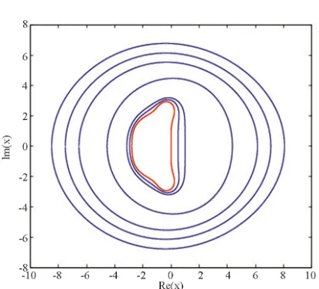
The corresponding families of stability regions are plotted in the complex x plane and displayed in Figure 1. Note that, in this figure, the horizontal and the vertical axes represent Re

 

x and Im

 

x , respectively. Clear-

ly, as shown in Figure 1, the stability region for the ETDRK4 scheme grows larger as . The red curve corresponds to the case , where the stability region of the ETDRK4 scheme coincides with that of the corresponding order fourth order Runge-Kutta (RK4) scheme.

y 

0

y

4. Numerical Results

method for solving the fifth order KdV equation. To show the efficiency of the present method, we report the relative infinity and root mean square norm errors of the solution defined by

1

1

max

, max

j j jN

j jN

u u

L

u 



 (28) We commence our analysis by choosing real negative

[image:6.595.58.287.71.278.2]

Figure 1. Stability regions in the complex x plane. The curv-

es correspond to , from the outer

curve to the inner curve respectively. The inner red curve corresponds to y = 0.

; ; ; ; ;

8 7 6 4 1 0.5

y      





 

2 1

2 2

1

,

N

j j j

N j j

u u

u

L 











(29)

respectively, where N is the number of interior points, j

u and u_j u

are the exact and computed values of the solution at point . j

In this paper, we consider two case studies depending on the set of parameters of (25) that provide multi-soliton solutions. We evaluate the performance the DSC al- gorithms for different time increment , spatial discre- tization , the support size of DSC kernels

t

N M and

regularization parameter  .

In our computation, the first set of parameters that we select are given by  5, 5, 5. In this case, the fifth order KdV Equation (11) is known as the Sawada- Kotera (SK) [2] equation and is given by

2

3 2 5

5 5 5

t x x x x x

u  uu  u u  u u u 0

,

. (30) The SK (30) admits multi-soliton solutions [31]. The derivation of these soliton solutions is beyond the scope of this paper. We only list them here for testing numeri- cal procedures purposes. Single and two soliton solutions are given by

 

, 6 ln



 

,



xx

u x t    x t  (31)

where

 

1

1 exp ,

   (32)

 

1

 

2 12



1



1 exp exp a exp ₂ ,

        (33)

respectively, with

















2 _{2 2}

5

2 _{2 2}

and i j i i j j

i i i i ij

i j i i j i

k k k k k k

k x k t a

k k k k k k

       

  

(34) In our computational work, we use the collocation points







1 , , 1 , ,



, .

1

i N

b a

x a x a i h x b h

N



     



 

(35) The SK equation possesses infinite conservation laws [31]. The first three conservation laws are given as fol- low

2 3

1 2 3

1

d , d , d ,

3 x

2

I u x I  u x I  u u x

  

 

   _  _

 







(36)

related to the mass, momentum and energy. The quan- tities I1, I2 and I3 are applied to measure the conser-

vation properties of the collocation scheme, calculated by

 

2

2 3

1 2 3

1

, , .

3

j j j j x j

j j

I h u I h u I h u u

  _



 

 

   _  _

 







(37) The second set of parameters are chosen as

10, 25, 20

      . This is well-known as the Kaup- Kupershmidt (KK) [3] equation

2

3 2 5

10 25 20 0.

t x x x x x

u  uu  u u  u u u  (38)

Multi-soliton solutions can be generated by the follow- ing nonlinear transformation of the dependent variable,

 

, 3 ln



 

,



2 xx.

u x t    x t _ (39)

For one soliton solution, the dependent variable func- tion is given by

 

 

5

1 1 1 1 1

1

1 exp exp 2 ,

16 k x k t 1

         (40)

For two soliton solutions, the dependent variable func- tion is

 

 

 

 

















1 2

2 12 1 2

12 1 2 1 2

2

12 1 2

1

1 exp exp exp 2

16

1 _{exp 2 exp}

16

exp 2 exp 2

exp 2 2 ,

a

b

b

1

  

  



   

 

   

  

 _    _

 

(41)

























4 2 2 4

1 1 2 2

12 2 2 2

1 2 1 1 2 2

2 2

1 2 1 1 2 2

12 2 2 2

1 2 1 1 2 2

2 2

, 2

. 16

k k k k

a

k k k k k k

k k k k k k

b

k k k k k k

 



  

  



  

2 (42)

The KK equation possesses infinite conservation laws [31], the first three are given as follows

2 3

1 2 3

1 1

d , d , d .

3 8

b b b

x

a a a

2

I  u x I  u x I   u  u x

 







 (43)

The quantities I1, I2 and I3 are applied to measure

the conservation properties of the collocation scheme, calculated by

 

2

2 3

1 2 3

1 1

, ,

3 8

j j j j x j

j j

I h u I h u I h u u

  _



 

 

   _  _

 







(44) In next sections, we study the propagation and the in- teraction of single and two soliton solutions, respectively.

4.1. Propagation of Single Solitons

In our numerical experiments, we first model the motion of a single soliton of the SK (30) and KK (38) equations. For the SK equation, the initial condition is taken from the exact solutions (32) and (31) at initial profile. Where- as for the KK equation, the initial condition is taken from the exact solutions (40) and (39) at initial profile. The boundary conditions in both cases are chosen so that



,



0 and

 

, 0

u  t  u t  . (45)

In the first computation, we would like to investigate the convergence of the DSC method with respect to the number of grid points N and the DSC bandwidth M. The values of the parameters used in our numerical expe- riments are: k₁0.4,₁0 and t0.001 in both cases of the SK and KK equations. In each case, the so-liton moves to the right across the space interval



100,100



x  when the time interval is t



0,1500



.

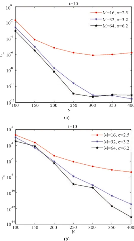
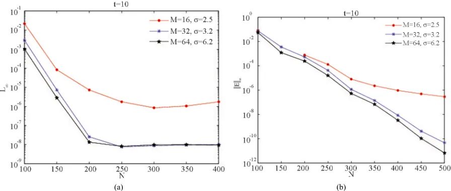
[image:7.595.311.536.84.488.2]

The choice of the DSC bandwidth M and the regular- izer parameter  is done according to the conditions (10). Hence if M 16 then  2.5h . If M 32 then  3.2h. If M 64 then  6.2h.

Figure 2 illustrates the convergence of the DSC with respect to the number of the grid points and the DSC bandwidth

N

M. We observe that numerical soliton solu- tions of the DSC method converge towards the exact so- liton solutions as the number of grid points increases. We remark that the convergence of the DSC method also relies on the bandwidth

N

M. The results in Figure 2 shows that the case gives a better convergence, the case gives the worst convergence, whereas when we have an intermediate convergence.

64 M 16 M

32



M

(a)

(b)

Figure 2. Convergence the DSC method for the propagation of single soliton solution of the SK (a) and the KK (b) equations at t10 with k10.4, 10 and δt0.001 and x 



100 100,



.

In fact when the bandwidth M is large, the DSC me- thod behaves like a global and detains exponential accu- racy, whereas for a small value of M, the DSC behaves like a local method such as finite difference methods. This result is stated by Theorem 2.1.

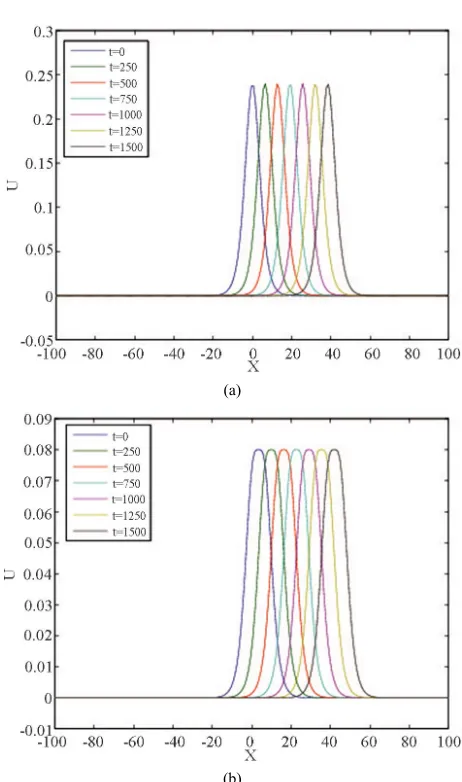
Figure 3 represents numerical propagation of one soli- ton solutions of the SK (a) and the KK (b) equations. These propagations occur for a long period of time with no spurious oscillations.

In the next experiment, we compute the error norms

L_, L₂ and conservation quantities I₁, I₂ and I₃.

The results are shown in Table 1 for one soliton solution of the SK equation and in Table 2 for one soliton solu-tion of the KK equasolu-tion.

(a)

[image:8.595.56.287.75.466.2]

(b)

Figure 3. Propagation of single soliton solution of the SK (a) and the KK (b) equations with k10.4 , 10 ,

, and

0.001

δt N200 x 



100 100,



.

is observed that throughout the simulation, the error norms and are of magnitude at a long pe- riod of time . Whereas the invariants ₁

L_ L₂

150



4

10

0

t I , I₂

and I₃ at a given time are equal to those of the ini-

tial value. Our scheme conserve, the mass, momentum and energy.

t

4.2. Interaction of Two Solitons

This computational work is related to the interaction of two soliton solutions of SK (30) and KK (38) equations having different amplitudes and travelling in the same direction. For the SK equation, the initial condition is ta- ken from the exact solutions (33) and (31) at initial pro- file; whereas for the KK equation, the initial condition is taken from the exact solutions (41) and (39) at initial pro- file. The boundary conditions in both cases are chosen so that

Table 1. Invariants and errors for a single soliton of the SK equation. k10.4 , 10 , N200 , δt0.1 and



100,



x  100 .

t L L2 I1 I2 I3

50 0 0 2.4000 0.3840 0.0123

[image:8.595.309.537.131.267.2]

250 2.9354E-7 6.4931E-7 2.4000 0.3840 0.0123 500 4.5926E-7 1.2687E-6 2.4000 0.3840 0.0123 750 1.1870E-6 2.6083E-6 2.4000 0.3840 0.0123 1000 7.2493E-6 1.6938E-5 2.4000 0.3840 0.0123 1250 3.8777E-5 9.0258E-5 2.4000 0.3840 0.0123 1500 3.0826E-4 7.1035E-4 2.4000 0.3840 0.0123

Table 2. Invariants and errors for a single soliton of the KK equation. k₁0.4, ₁0, N200,δt0.1 and



100,100



x  .

t L L2 I1 I2 I3

50 0 0 1.2000 0.0730 0.0015

250 2.4116E-7 5.0563E-7 1.2000 0.0730 0.0015 500 4.3930E-7 9.6785E-7 1.2000 0.0730 0.0015 750 6.4347E-7 1.4086E-6 1.2000 0.0730 0.0015 1000 7.2969E-7 1.8528E-6 1.2000 0.0730 0.0015 1250 1.1567E-6 2.3038E-6 1.2000 0.0730 0.0015 1500 1.2106E-6 2.7218E-6 1.2000 0.0730 0.0015



,



0

 

, 0

u t  and u t  . (46)

To allow the interaction to occur, the experiment was run from t0 to 400 in the region



100,100



1

k 

. Fig- ure 4 shows the interaction of two soliton solutions of the SK (top) and KK (bottom) equations for ,

,

0.4

2 0.6

k  ₁0 , ₂ 30, N200,t0.001 and



10



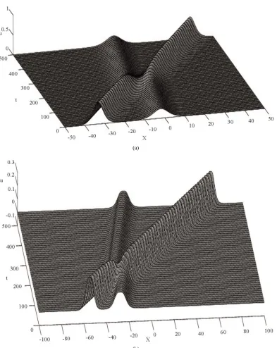
x  0,100 . It can be seen that the faster pulse in-

teracts with and emerges ahead of the lower pulse with the shape and velocity of each soliton retained.

We also investigate the convergence of the DSC me- thod with respect to the number of the grid points and the DSC bandwidth

N M as we did in the case of one soliton solutions.

All the results are shown in Figure 5. We observe that numerical soliton solutions obtained by means of the DSC method converge to the exact soliton solutions as the number of grid points increases. We also ob- serve that the convergence of the DSC method relies on the bandwidth

N

M. The results on Figure 5 show that the case M64 gives a better convergence, the case

16

[image:8.595.310.538.326.465.2]

(a)

[image:9.595.105.498.81.575.2]

(b)

Figure 4. Interaction of two soliton solutions of the SK (top) and the KK (bottom) equations with k₁0.4, k20.6, 10,

, , and

230

 N200 δt0.001 x 



100 100,



. 32

M  we have an intermediate convergence. In fact when the bandwidth M is large, the DSC method be- haves like a global and detains exponential accuracy, whereas for a small value of M, the DSC behaves like a local method such as finite difference methods.

In addition, we compute the error norms , 2 and

conservation quantities 1

L_ L

I , I₂ and I₂ are computed.

The result are shown in Table 3 for two soliton solutions of the SK equation and in Table 4 for two soliton so-

lutions of the KK equation.

From the numerical results given in Table 3 it is ob- served that throughout the simulation, the error norms

L_ and ₂ are of magnitude at a long period of

time , whereas the error norms and 2 (Table

4) are of magnitude

L

0

5

10

40 L_ L

8

10 _{at a long period of time. The}

invariants I1, I2 and I2 at a given time are equal

to those of the initial value. Numerical checks on the con- servation mass, momentum and energy show that the

[image:10.595.75.523.87.277.2]

(a) (b)

[image:10.595.57.286.364.469.2]

Figure 5. Convergence the DSC method for the interaction of two soliton solutions of the SK (a) and the KK (b) equations with k₁0.4, k₂0.6, ₁0, ₂30,δt0.001 and x 



100 100,



.

Table 3. Invariants and errors for interaction of two soli- tons of the SK equation. k10.4 , k20.6 , 10 ,

230

 , δt0.001, N200, x 



100 100,



.

t L L2 I1 I2 I3

50 0 0 6.0000 1.6799 0.1056

[image:10.595.57.286.529.632.2]

100 2.3576e-008 4.6137e-008 6.0000 1.6736 0.1056 200 2.6207e-007 6.5108e-007 6.0000 1.5118 0.1056 300 7.2470e-007 2.2323e-006 6.0000 1.6552 0.1056 400 7.7486e-005 2.3119e-004 6.0000 1.6796 0.1056

Table 4. Invariants and errors for interaction of two soli- tons of the KK equation. k10.4 , k20.6 , 10 ,

230

 , δt0.001, N450, x 



100 100,



.

t L L2 I1 I2 I3

50 0 0 3.0000 0.3194 0.0132

100 4.6168e-009 5.2241e-009 3.0000 0.3194 0.0132 200 2.6397e-009 3.5804e-009 3.0000 0.3194 0.0132 300 2.6443e-009 4.1965e-009 3.0000 0.3194 0.0132 400 8.4855e-009 1.2871e-008 3.0000 0.3194 0.0123

three quantities remain constant with respect to time.

5. Conclusion

We studied the application of the combined DSC scheme in space discretization and the ETDRK4 for time discre- tization to solve the SK and KK equations. We consid- ered the case of the propagation of a single soliton and

the interaction of two solitons. Numerical results showed that the DSC method converges exponentially with re- spect to the number of grid points N and the bandwidth

M. Numerical checks on the conservation mass, mo- mentum and energy revealed that the three quantities re- main constant with respect to time . The DSC scheme is a robust and reliable numerical method of the fifth or- der KdV equation. We are currently investigating the uti- lity of the DSC method to solve the GRLW equation.

t

6. Acknowledgements

E. Pindza acknowledges the financial support from Brad Welch through RidgeCape.

REFERENCES

[1] P. D. Lax, “Integrals of Nonlinear Equations of Evolution and Solitary Waves,” Communications on Pure and Ap- plied Mathematics, Vol.21, No. 5, 1968, pp. 467-490.

http://dx.doi.org/10.1002/cpa.3160210503

[2] K. Sawada and T. Kotera, “A Method for Finding N- Soliton Solutions for the KdV Equation and KdV-Like Equations,” Progress of Theoretical Physics, Vol. 51, No.

5, 1974, pp. 1355-1367.

http://dx.doi.org/10.1143/PTP.51.1355

[3] A. P. Fordy and J. Gibons, “Some Remarkable Nonlinear Transformations,” Physics Letters, Vol. A75, No. 5, 1980,

p. 325. http://dx.doi.org/10.1016/0375-9601(80)90829-4 [4] M. Ito, “An Extension of Nonlinear Evolution Equations

of the KdV (mKdV) Type to Higher Orders,” Journal of the Physical Society of Japan, Vol. 49, 1980, pp. 771-778.

http://dx.doi.org/10.1143/JPSJ.49.771

Analysis, Vol. 41, No. 5, 2003, pp. 1595-1619.

http://dx.doi.org/10.1137/S0036142902410271

[6] J. Shen and L. L. Wang, “Laguerre and Composite Leg- endre-Laguerre Dual-Petrov-Galerkin Methods for Third- Order Equations,” DCDS-B, Vol. 6, No. 6, 2006, pp.

1381-1402. http://dx.doi.org/10.3934/dcdsb.2006.6.1381 [7] J. M. Yuan, J. Shen and J. Wu, “A dual-Petrov-Galerkin

Method for the Kawahara-Type Equation,” Journal of Sci- entific Computing, Vol. 34, No. 1, 2008, pp. 48-63.

http://dx.doi.org/10.1007/s10915-007-9158-4

[8] G. W. Wei, “Discrete Singular Convolution for the Fok- ker-Planck Equation,” Journal of Chemical Physics, Vol.

110, 1999, pp. 8930-8942. http://dx.doi.org/10.1063/1.478812

[9] W. Bao, F. Sun and G. W. Wei, “Numerical Methods for the Generalized Zakharov System,” Journal of Computa- tional Physics, Vol. 190, No. 1, 2003, pp. 201-228.

http://dx.doi.org/10.1016/S0021-9991(03)00271-7 [10] G. W. Wei, Y. B. Zhao and Y. Xiang, “Discrete Singular

Convolution and Its Application to the Analysis of Plates with Internal Supports. Part 1: Theory and Algorithm,”

International Journal Numerical Methods in Engineering,

Vol.55, No. 8, 2002, pp. 913-946. http://dx.doi.org/10.1002/nme.526

[11] G. W. Wei, “Vibration Analysis by Discrete Singular Con- volution,” Journal of Sound Vibration, Vol. 244, No. 3,

2001, pp. 535-553.

http://dx.doi.org/10.1006/jsvi.2000.3507

[12] G. W. Wei, “A New Algorithm for Solving Some Mecha- nical Problems,” Computational Methods in Applied Me- chanical Engineering, Vol. 190, No. 15, 2001, pp. 2017-

2030. http://dx.doi.org/10.1016/S0045-7825(00)00219-X [13] Y. C. Zhou and G. W. Wei, “High-Resolution Conjugate

Filters for the Simulation of Flows,” Journal of Computa- tional Physics, Vol. 189, No. 1, 2003, pp. 150-179.

[14] G. Bao, G. W. Wei and S. Zhao, “Numerical Solution of the Helmholtz Equation with High Wave Numbers,” In- ternational Journal of Numerical Methods in Engineering,

Vol. 59, No. 3, 2004, pp. 389-408. http://dx.doi.org/10.1002/nme.883

[15] G. Bao, G. W. Wei and S. Zhao, “Local Spectral Time- Domain Method for Electromagnetic Wave Propagation,”

Optic Letters, Vol. 28, No. 7, 2003, pp. 513-515.

http://dx.doi.org/10.1364/OL.28.000513

[16] Z. J. Hou and G. W. Wei, “A New Approach for Edge De- tection,” Pattern Recognition, Vol. 35, No. 7, 2002, pp.

1559-1570.

http://dx.doi.org/10.1016/S0031-3203(01)00147-9 [17] E. Pindza and E. Maré, “Discrete Singular Convolution

and Exponential Time Integrators for Solving the Gener- alized Korteweg-de Vries Equation,” Technical Report UPWT 2013/14, University of Pretoria, Pretoria. [18] S. Y. Yang, Y. C. Zhou and G. W. Wei, “Comparison of

the Discrete Singular Convolution Algorithm and the Fou- rier Pseudospectral Methods for Solving Partial Differen-

tial Equations,” Computer Physics Communications, Vol.

143, No. 2, 2002, pp. 113-135.

http://dx.doi.org/10.1016/S0010-4655(01)00427-1 [19] G. W. Wei, Y. B. Zhao and Y. Xiang, “A Novel Approach

for the Analysis of High Frequency Vibrations,” Journal of Sound and Vibration, Vol. 257, No. 2, 2002, pp. 207-

246. http://dx.doi.org/10.1006/jsvi.2002.5055

[20] A. K. Kassam and L. N. Trefethen, “Fourth-Order Time Stepping for Stiff PDEs,” SIAM Journal of Scientific Computing, Vol. 26, No. 4, 2005, pp. 1214-1233.

http://dx.doi.org/10.1137/S1064827502410633

[21] L. N. Trefethen and H. M. Gutknecht, “The Carathéodory- Fejér Method for Real Rational Approximation,” SIAM Journal on Numerical Analysis, Vol. 20, No. 2, 1983, pp.

420-436. http://dx.doi.org/10.1137/0720030

[22] G. W. Wei, “Discrete Singular Convolution for the Sine- Gordon Equation,” Physica D, Vol. 137, No. 3, 2000, pp.

247-259.

http://dx.doi.org/10.1016/S0167-2789(99)00186-4 [23] L. W. Qian, “On the Regularized Whittaker-Kotel’nikov-

Shannon Sampling Formula,” Proceedings of American Mathematical Society, Vol. 131, No. 4, 2003, pp. 1169-

1176. http://dx.doi.org/10.1090/S0002-9939-02-06887-9 [24] R. X. Yao, C. Z. Qu and Z. B. Li, “On Properties of New

Parameterized 5th-Order Nonlinear Evolution Equation,”

Chaos, Solitons and Fractals, Vol.21, No. 5, 2004, pp.

1145-1152. http://dx.doi.org/10.1016/j.chaos.2003.12.078 [25] E. Pindza, “Spectral Difference Methods for Solving Equ- ation of the KdV Hierarchy,” MSc Thesis, University of Stellenbosch, Stellenbosch, 2008.

[26] B. Minchev and W. Wright, “A Review of Exponential In- tegrators for First Order Semi-Linear Problems,” Techni- cal Report 2, The Norwegian University of Science and Technology, 2005.

[27] S. M. Cox and P. C. Matthews, “Exponential Time Diffe- rencing for Stiff Systems,” Journal of Computational Phy- sics, Vol. 176, No. 2, 2002, pp. 430-455.

http://dx.doi.org/10.1006/jcph.2002.6995

[28] Y. Saad, “Analysis of Some Krylov Subspace Approxima- tions to the Matrix Exponential Operator,” SIAM Journal of Numerical Analysis, Vol. 29, No. 1, 1992, pp. 209-228.

http://dx.doi.org/10.1137/0729014

[29] M. Hochbruck and C. Lubich, “On Krylov Subspace Ap- proximations to the Matrix Exponential Operator,” SIAM Journal of Numerical Analysis, Vol. 34, No. 5, 1997, pp.

1911-1925.

http://dx.doi.org/10.1137/S0036142995280572

[30] T. Schmelzer and L. N. Trefethen, “Evaluating Matrix Functions for Exponential Integrators via Carathéodory- Fejér Approximation and Contour Integrals,” Electronic Transactions on Numerical Analysis, Vol. 29, 2007, pp.

1-18.