A Group based Time Quantum Round Robin Algorithm using Min Max Spread Measure

(1)

A Group based Time Quantum Round Robin Algorithm

using Min-Max Spread Measure

Sanjaya Kumar Panda

Department of CSE

NIT, Rourkela

Debasis Dash

Department of CSE

NIT, Rourkela

Jitendra Kumar Rout

Department of CSE

NIT, Rourkela

ABSTRACT

Round Robin (RR) Scheduling is the basis of time sharing environment. It is the combination of First Come First Served (FCFS) scheduling algorithm and preemption among processes. It is basically used in a time sharing operating system. It switches from one process to another process in a time interval. The time interval or Time Quantum (TQ) is fixed for all available processes. So, the larger process suffers from Context Switches (CS). To increase efficiency, we have to select different TQ for processes. The main objective of RR is to reduce the CS, maximize the utilization of CPU and minimize the turn around and the waiting time. In this paper, we have considered different TQ for a group of processes. It reduces CS as well as enhancing the performance of RR algorithm. TQ can be calculated using min-max dispersion measure. Our experimental analysis shows that Group Based Time Quantum (GBTQ) RR algorithm performs better than existing RR algorithm with respect to Average Turn Around Time (ATAT), Average Waiting Time (AWT) and CS.

General Terms

Operating System, Scheduling

Keywords

Round Robin, Time Quantum, Min-Max, Ready Queue, Group Based Time Quantum

1. INTRODUCTION

In the time sharing environment, the processes are sharing CPU time one after another. The time is referred as time slice or time interval or TQ. After the specified TQ is expired, the CPU time is used by another process. If a process completes its execution before TQ expired, then next process is assigned to the processor. When TQ is very less, the response time and the context switching are more. Normally, TQ is in between 10 to 100 milliseconds [7]. Context switch is the time required to switch from one process to another process. The queue used in RR is a circular queue [2].

RR is the most prominent scheduling algorithm in time sharing systems. It gives equal priority to each process present in RQ. The response time of processes is reduced into a greater extent. The main objective of RR is to minimize the turn around time and the waiting time, maximize the CPU utilization and reduce the CS [3]. CS is an overhead to the OS. Scheduling algorithms are divided into two types: preemptive and non-preemptive. In preemptive, higher priority process can preempt the current process in the middle of execution. The current process is moved to RQ. But, Non-preemptive process cannot be released in the middle of execution. A preemptive algorithm may have more CS than Non-preemptive algorithm. RR is a Non-preemptive scheduling algorithm.

Scheduling is done using three schedulers: Long term, Short term and Medium term. Initially, the process is in the spool disk. Long term scheduler is responsible for loading the process from the spool disk to the RQ [2] [4]. When the main memory is free, one of the processes present in the RQ is loaded into main memory. The short term scheduler is responsible for this queuing action. The medium term scheduler is used for I/O execution. The process may require an I/O operation. For I/O execution, the process is moved from the main memory to I/O waiting queue. After I/O operation is over, it is again moved from waiting queue to the ready queue.

CPU scheduling determines which process is allocated to main memory. Each scheduling algorithm is trying to optimize the ATAT, AWT and Average Response Time (ART) [4] [5] [6]. CPU utilization and throughput are also used to measure the performance of an algorithm.

The remaining part of this paperwork is organized as follows. Related work is presented in section 2. The preliminaries are shown in Section 3. Section 4 elaborates the proposed GBTQ RR algorithm with flow chart. The performance analysis is presented in Section 5. We conclude our work in Section 6.

2. RELATED WORK

Many researchers have been proposed various methods to improve CPU scheduling. As TQ is inversely proportional to response time, choosing a high TQ will not be wise. Also, static time quantum leads to more CS. So, we have to design such an algorithm which chooses TQ properly as well as CS is very less.

It is better to repeatedly adjust the TQ. Matarneh [6], Panda et al. [1], Bhoi et al. [3] proposes an algorithm based on TQ set. They use a different mathematical measure to choose the TQ. Mostafa et al. [5] uses integer programming to decide the TQ. The TQ is not a too big or too small value. It also reduces the CS.

Noon et al. [4] presents a dynamic TQ mechanism. It also overcomes the demerit of RR such as the fixed TQ problem, CS etc. Bhunia [9] et al. proposes an enhanced version of feedback scheduling. It focuses on the lower priority queue process.

Yuan et al. [10] proposes Fair Round-Robin (FRR). It has a low-complexity scheduler. It gives good short term fairness than STRR [10] [11].

3. PRELIMINARIES

(2)

Robin (MMRR) [1], Self Adjustment Round Robin (SARR) [6], Virtual Time Round Robin (VTRR) [8], Subcontrary Mean Dynamic Round Robin (SMDRR) [3] etc. The algorithms are listed below. All units are in seconds.

3.1 FCFS

It seems like a ticket counter. The process which arrives first in RQ is served first. It is a non-preemptive scheduling algorithm. It means processor cannot release the process before its execution is over. It suffers from Starvation. The process present in the last of RQ has to wait until all process execution is over. So, the TAT and WT are more.

3.2 SJF

The algorithm gives priority to shortest process available in RQ. It is also a non-preemptive scheduling algorithm. The process has high Burst Time (BT) suffers most in this algorithm. This type of suffering is called as Aging.

3.3 SRTF

It is a preemptive scheduling algorithm. Like SJF, it chooses shortest process first. But, if a new process arrives in RQ, then it compares the new process with the running process. The process which takes less remaining time will occupy the CPU first.

3.4 HRRN

The algorithm gives priority to the process which holds the highest response ratio (HRR). The response ratio can be calculated using the equation 1 [2].

HRR = Turn around Time / Response Time (1)

3.5 MMRR

It is also a preemptive algorithm. The TQ is repeatedly adjusted in each iteration. It uses Min-Max dispersion measure. The TQ can be calculated using the equation 2 [1]. TQ = Maximum Burst Time - Minimum Burst Time (2)

3.6 SARR

Like MMRR, the TQ is adjusted in SARR. It uses Median to repeatedly adjust the TQ. If the TQ is less than 25, then it automatically sets the TQ to 25 [6]. It is also reducing the context switch between processes.

3.7 VTRR

It is based on a fair queuing algorithm. O (1) time is required to schedule a client for execution. It was implemented on Linux platform [8].

3.8 SMDRR

It uses harmonic mean or subcontrary mean to adjust the TQ. Based on the burst time, it will calculate the harmonic mean. Then, it selects the TQ [3].

4. PROPOSED ALGORITHM

4.1 Notations

Notation Definition RQ Ready Queue Q1 First Quartile

Q2 Second Quartile

Q3 Third Quartile

N Total Number of Processes BT [Pi] Burst Time of Process i

RQi Ready Queue i

TQ [RQi] Time Quantum for Ready Queue i

MaxBT[Pk] Maximum Burst Time Process k

MinBT[Pl] Minimum Burst Time Process l

α Threshold

TQnew [RQi] New Time Quantum for Ready Queue i

4.2 Descriptions

In our GBTQ algorithm, the processes are sorted in RQ. The quartile measure is used to form a group among the processes. The Q1 is the 25% of the data set. The Q2 (or median) is the

50% of the data set. Finally, the Q3 is the 75% of the data set.

It is used in our algorithm because the too short TQ may lead to more CS. Alternatively, the too large TQ may lead to starvation. Based on the CPU BT, the processes are formed four groups. Each group has different TQ. Different TQ is used to reduce CS. As shown in my earlier paper [1], Min-Max dispersion or spread measure was taken to calculate the TQ. The formula is shown in equation 2. It may suffer from CS, if the difference between MaxBT and MinBT is very less. So, in the proposed algorithm, α is used as a threshold to reduce CS. Finally, the TQ is assigned to each group. The process is continued until RQ is empty. After execution of all processes, ATAT, AWT and CS are calculated.

4.3 Performance Measure

4.3.1 Turn Around Time (TAT)

It is the overall time a process requires for execution. It can be calculated using the equation 3. The average of all process is termed as ATAT. It can be calculated using equation 4. TAT = Finish Time – Arrival Time (3)

(4)

4.3.2 Waiting Time (WT)

It is the queuing delay time require for execution. It may be the time spent in RQ or I/O queue. Normally, it can be calculated using the equation 5. The average WT of all process is termed as AWT. It can be calculated using equation 6.

WT = Start Time – Arrival Time (5)

4.3.3 Context Switch (CS)

(3)

Pj is more priority over Pi. Ts (Pi) denote the start time of Pi

and Te (Pj) denotes the finish time of Pj. Let us assume that Pi

immediately follows Pj. Then, the CS can be calculated using

equation 7.

CS = Te (Pj) - Ts (Pi) (7)

4.4 Algorithm

1. Sort the processes present in the RQ. 2. while (RQ != NULL)

3. Calculate Q1, Q2, Q3.

4. for i = 1 to N 5. if BT [Pi] ≤ Q1

6. Place it in RQ1.

7. else if (BT [Pi] > Q1 && BT[Pi] ≤ Q2)

8. Place it in RQ2.

9. else if (BT [Pi] > Q2 && BT[Pi] ≤ Q3)

10. Place it in RQ3.

11. else (BT[Pi] > Q3)

12. Place it in RQ4.

13. end if 14. end for 15. for i = 1 to 4

16. Set TQ [RQi] = MaxBT[Pk] – MinBT[Pl]

17. if (TQ [RQi] > α)

18. Set TQnew [RQi] = TQ [RQi]

19. else

20. Set TQnew [RQi] = α

21. end if 22. end for 23. for i = 1 to N 24. if (Pi € RQ1)

25. Pi ← TQnew [RQ1]

26. else if (Pi € RQ2)

28. else if (Pi € RQ3)

30. else

32. end if 33. end for 34.Update N. 35. if (N != NULL) 36. Go to Step 23. 37. else

38. Go to Step 40. 39. end if

[image:3.595.301.575.81.541.2]

40. Calculate ATAT, AWT, NCS. 41.end while

Fig. 1: Proposed Algorithm

4.5 Flow Chart

Fig. 2: Flowchart for GBTQ

5. EXPERIMENTAL RESULTS

5.1 Illustrations

We have considered different cases by varying arrival time and burst time. The processes are numbered as P1, P2,P3, … ,

PN where N is the number of processes available in RQ. The

below case cover both uniform (U) and non-uniform (NU) BT. The specification of different cases is listed in Table 1.

Table 1. Case Specifications

Case No.

N Arrival Time

TQ (α)

BT Range

U / NU

1 10 No 20 7-200 NU

2 4 No 20 11-95 NU

3 4 No 20 81-84 U

4 8 No 20 61-68 U

5 5 Yes 20 7-75 NU

[image:3.595.63.522.91.721.2]

(4)

5.1.1 Case 1

[image:4.595.309.555.70.191.2]

Let us assume that 10 processes (with AT = 0) have arrived in RQ. The Table 2 shows the AT and BT of each process. In this case, the threshold value is assumed to be α = 20 for processes. The Table 3 shows the comparison of RR and GBTQ respectively. The Figure 3 and 4 shows the gantt chart for RR and GBTQ respectively.

Table 2. Processes with Burst Time (Case I)

Process Arrival Time

Burst Time

P1 0 7

P2 0 15

P3 0 24

P4 0 84

P5 0 123

P6 0 145

P7 0 150

P8 0 175

P9 0 180

[image:4.595.90.245.173.374.2]

P10 0 200

Table 3. Comparison of RR and GBTQ (Case I)

Algorithm TQ ATAT AWT CS

RR 20 681.3 571 58

GBTQ 20,39,30,20 610.9 498.6 44

P1 P2 P3 P4 P5 P6 P7 P8 P9 P10 P3 P4

7 22 42 62 82 102 122 142 162 182 186 206 P5 P6 P7 P8 P9 P10 P4 P5 P6 P7 P8 P9

226 246 266 286 306 326 346 366 386 406 426 446 P10 P4 P5 P6 P7 P8 P9 P10 P4 P5 P6 P7

466 486 506 526 546 566 586 606 610 630 650 670 P8 P9 P10 P5 P6 P7 P8 P9 P10 P5 P6 P7

690 710 730 750 770 790 810 830 850 853 873 893 P8 P9 P10 P6 P7 P8 P9 P10 P8 P9 P10

913 933 953 958 968 988 1008 1028 1043 1063 1103 Fig. 3: Gantt chart for RR

P1 P2 P3 P4 P5 P6 P7 P8 P9 P10 P3 P4

7 22 42 81 120 150 180 210 230 250 254 293

P5 P6 P7 P8 P9 P10 P4 P5 P6 P7 P8 P9

332 362 392 422 442 462 468 507 537 567 597 617 P10 P5 P6 P7 P8 P9 P10 P6 P7 P8 P9 P10

637 643 673 703 733 753 773 798 828 858 878 898 P8 P9 P10 P9 P10 P9 P10 P9 P10 P10

923 943 963 983 1003 1023 1043 1063 1083 1103 Fig. 4: Gantt chart for GBTQ

5.1.2 Case 2

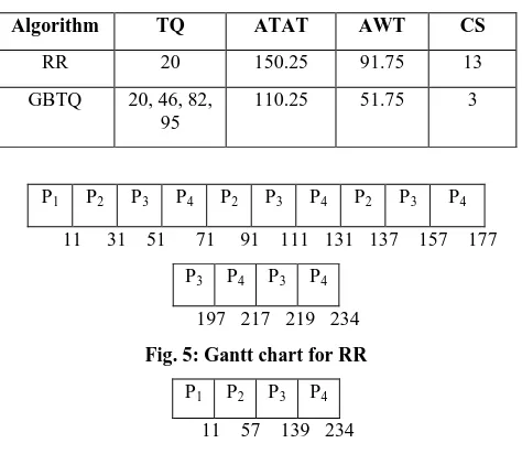
[image:4.595.345.509.299.404.2]

Let us assume that 4 processes (with AT = 0) have arrived in RQ. The Table 4 shows the AT and BT of each process. Like Case 1, the threshold is assumed to be α = 20 for processes. The Table 5 shows the comparison of RR and GBTQ respectively. The Figure 5 and 6 shows the gantt chart for RR and GBTQ respectively.

Table 4. Processes with Burst Time (Case II)

Burst Time

P1 0 11

P2 0 46

P3 0 82

[image:4.595.43.296.396.705.2]

P4 0 95

Table 5. Comparison of RR and GBTQ (Case II)

RR 20 150.25 91.75 13

GBTQ 20, 46, 82, 95

110.25 51.75 3

P1 P2 P3 P4 P2 P3 P4 P2 P3 P4

11 31 51 71 91 111 131 137 157 177 P3 P4 P3 P4

197 217 219 234 Fig. 5: Gantt chart for RR

P1 P2 P3 P4

11 57 139 234 Fig. 6: Gantt chart for GBTQ

5.1.3 Case 3

[image:4.595.312.549.428.634.2]

(5)

Table 6. Processes with Burst Time (Case III)

Table 7. Comparison of RR and GBTQ (Case III)

RR 20 325 242.5 19

GBTQ 81, 82, 83, 84

205 122.5 3

P1 P2 P3 P4 P5 P6 P7 P8 P1 P2

20 40 60 80 100 120 140 160 180 200 P3 P4 P1 P2 P3 P4 P1 P2 P3 P4

220 240 260 280 300 320 321 323 326 330 Fig. 7: Gantt chart for RR

P1 P2 P3 P4

81 163 246 330 Fig. 8: Gantt chart for GBTQ

5.1.4 Case 4

Let us assume that 8 processes (with uniform BT) have arrived in RQ. The Table 8 shows the AT and BT of each process. In this case, assumed value for threshold is α = 20 for processes. The Table 9 shows the comparison of RR and GBTQ respectively. The Figure 9 shows the gantt chart for RR as well as GBTQ.

Table 8. Processes with Burst Time (Case IV)

Burst Time

P1 0 61

P2 0 62

P3 0 63

P4 0 64

P5 0 65

P6 0 66

P7 0 67

P8 0 68

Table 9. Comparison of RR and GBTQ (Case IV)

RR 20 495 430.5 31

GBTQ 20, 20, 20, 20 495 430.5 31

P1 P2 P3 P4 P5 P6 P7 P8 P1 P2 P3 P4

20 40 60 80 100 120 140 160 180 200 220 240 P5 P6 P7 P8 P1 P2 P3 P4 P5 P6 P7 P8

260 280 300 320 340 360 380 400 420 440 460 480

P1 P2 P3 P4 P5 P6 P7 P8

481 483 486 490 495 501 508 516 Fig. 9: Gantt chart for RR and GBTQ

5.1.5 Case 5

Let us assume that 5 processes (with AT) have arrived in RQ. The Table 10 shows the AT and BT of each process. In this case, value of threshold is assumed to be α = 20 for processes. The Table 11 shows the comparison of RR and GBTQ respectively. The Figure 10 and 11 shows the gantt chart for RR and GBTQ respectively.

Table 10. Processes with Burst Time (Case V)

Burst Time

P1 0 7

P2 5 14

P3 15 55

P4 50 75

P5 75 23

Table 11. Comparison of RR and GBTQ (Case V)

RR 20 87.4 52.6 8

GBTQ 20, 20, 55, 75

85.8 51 4

P1 P2 P3 P3 P4 P3 P5 P4 P5 P4 P4

7 21 41 61 81 96 116 136 139 159 174 Fig. 10: Gantt chart for RR

P1 P2 P3 P4 P5 P5

7 21 76 151 171 174 Fig. 11: Gantt chart for GBTQ Process Arrival

Time

Burst Time

P1 0 81

P2 0 82

P3 0 83

(6)

5.1.6 Case 6

[image:6.595.315.544.106.236.2]

Let us assume that 7 processes (with AT) have arrived in RQ. The Table 12 shows the AT and BT of each process. In this case, assumed threshold value is α = 20 for processes. The Table 13 shows the comparison of RR and GBTQ respectively. The Figure 12 and 13 shows the gantt chart for RR and GBTQ respectively.

Table 12. Processes with Burst Time (Case VI)

Burst Time

P1 0 24

P2 17 48

P3 35 65

P4 50 74

P5 70 89

P6 80 100

P7 130 150

Table 13. Comparison of RR and GBTQ (Case VI)

RR 20 333.43 254.86 26

GBTQ 24, 20, 20, 150

327.71 249.14 25

P1 P2 P3 P2 P4 P3 P5 P6 P4 P7 P3 P5 P6

24 48 68 92 112 132 152 172 192 212 232 252 272 P4 P7 P3 P5 P6 P4 P7 P5 P6 P7 P5 P6 P7

292 312 317 337 357 371 391 411 431 451 460 480 550 Fig. 12: Gantt chart for RR

P1 P2 P1 P3 P2 P4 P3 P5 P6 P2 P4 P3

20 40 44 64 84 104 124 144 164 172 192 212 P7 P5 P6 P4 P3 P7 P5 P6 P4 P5 P6 P7

232 252 272 292 297 317 337 357 371 391 411 431 P5 P6 P7

[image:6.595.86.247.174.331.2]

440 460 550 Fig. 13: Gantt chart for GBTQ

5.2 Experiments

In Section 5.1, six cases are explained. In each case, we compare the proposed GBTQ algorithm with the existing RR algorithm. Both algorithms give the same result in case 4. The experiments show that the proposed algorithm is better than RR algorithm in terms of ATAT, AWT and CS. Performance

metrics of different cases are shown in Figure 14, Figure 15 and Figure 16 respectively.

[image:6.595.42.294.174.674.2]

Fig. 14: Comparison of Turn Around Time

[image:6.595.314.543.278.409.2]

Fig. 15: Comparison of Waiting Time

Fig. 16: Comparison of Context Switch

6. CONCLUSION

Scheduling is a major area in the operating system. Scheduling process may be user process or kernel process. A process may demand for more I/O than the CPU. So, we need an efficient scheduling to compensate CPU process with I/O process. In the proposed GBTQ algorithm, we are focusing on CPU process only. A group based TQ is proposed in this algorithm. Each group has different TQ. This algorithm reduces starvation as well as CS.

In the future, we can extend it to I/O processes. Deadline constraints may be considered as a part of research. We can

0 200 400 600 800

1 2 3 4 5 6

RR

GBTQ

0 100 200 300 400 500 600

1 2 3 4 5 6

RR

GBTQ

0 20 40 60 80

1 2 3 4 5 6

RR

[image:6.595.315.542.447.579.2]

(7)

explore the idea of RR to multi-processor (homogeneous or non-homogeneous) environment.

7. REFERENCES

[1] S. K. Panda and S. K. Bhoi, “An Effective Round Robin Algorithm using Min-Max Dispersion Measure”, International Journal on Computer Science and Engineering, Vol. 4, No. 1, Jan. 2012, pp. 45-53. [2] P. Balakrishna Prasad, “Operating Systems”, Scitech

Publications, Second Edition, Sep. 2008, ISBN- 9788188429608.

[3] S. K. Bhoi, S. K. Panda and D. Tarai, “Enhancing CPU Performance using Subcontrary Mean Dynamic Round Robin (SMDRR) Scheduling Algorithm”, Journal of Global Research in Computer Science, Vol. 2, No. 12, Dec. 2011, pp. 17-21.

[4] A. Noon, A. Kalakech and S. Kadry, “A New Round Robin Based Scheduling Algorithm for Operating Systems: Dynamic Quantum Using the Mean Average”, International Journal of Computer Science Issues, Vol. 8, Issue 3, No. 1, May 2011, pp. 224-229.

[5] S. M. Mostafa, S. Z. Rida and S. H. Hamad, “Finding Time Quantum of Round Robin CPU Scheduling Algorithm in General Computing Systems using Integer Programming”, International Journal of Research and Reviews in Applied Sciences, Vol. 5, No. 1, Oct. 2010, pp. 64-71.

[6] R. J. Matarneh, “Self-Adjustment Time Quantum in Round Robin Algorithm Depending on Burst Time of the Now Running Processes”, American Journal of Applied Sciences, Vol. 6, No. 10, 2009, pp. 1831-1837.

[7] A. Silberschatz, P. B. Galvin and G. Gagne, “Operating System Concepts”, John Wiley & Sons, Sixth Edition, 2002, ISBN 9971-51-388-9.

[8] J. Nieh, C. Vaill and H. Zhong, “Virtual-Time Round-Robin: An O(1) Proportional Share Scheduler” Proceedings of the USENIX Annual Technical Conference, Boston, Massachusetts, USA, Jun. 2001, pp. 25-30.

[9] A. Bhunia, “Enhancing the Performance of Feedback Scheduling”, International Journal of Computer Applications, Vol. 18, No. 4, Mar. 2011, pp. 11-16. [10]X. Yuan and Z. Duan, “Fair Round-Robin: A

Low-Complexity Packet Scheduler with Proportional and Worst-Case Fairness”, IEEE Transactions on Computers, Vol. 58, No. 3, Mar. 2009, pp. 365-379.