Neural Network based Sensor Fault Detection for
Flight Control Systems
Seema Singh
Associate Professor,
Dept. of Electronics &Communication BMS Institute of Technology
Bangalore, India
T. V. Rama Murthy
Senior Professor,
Dept. of Electronics &Communication Reva Institute of Technology & Management
Bangalore, India
ABSTRACT
Sensor fault in aircraft is detected based on two different approaches. The first approach, well documented in literature, is based on algorithmic method dealing with Luenberger observers. The second approach, which is followed in this paper, is based on Knowledge based neural network fault detection (KBNNFD). KBNNFD uses gradient descent back propagation training algorithm of neural network. A C-Star controller of F8 aircraft model, which improves the handling qualities, is used for validation of the KBNNFD. Neural network is trained with certain features of F8 aircraft model and C-Star controller enabling it to detect the faulty sensor.A comparative analysis of both the methods is done for various cases of stuck fault of the sensor for flight control system. Nz (Normal acceleration) sensor failure was considered because of its importance in C-Star controller. Knowledge-based approach of neural network, used in this work, has come out with results indicating that it takes less time to detect the faulty Nz sensor during transition, steady state and also in the presence of random noise. Results show improvement when compared to algorithmic methods with regard to the time taken to detect faults and ability to detect sensor faults especially near steady state. Investigations have been carried out using Matlab and Simulink.
General Terms
x : State space matrix of Aircraft model, [q Nzδe ]T u : Input; Elevator command (rad)
q, Nz, δe :Aircraft states; pitch rate (rad), Normal acceleration (ft/s2), Elevator position (rad) y : Output, [2x1]; [q, Nz]
A,B,C,D : State space matricesspecifications of Aircraft longitudinal model.
Keywords
Gradient descent back propagation algorithm, Knowledge base Neural Network, Aircraft Flight Control system, C-Star Controller, Stuck sensor fault, Simulink.
1.
INTRODUCTION
FAULT detection and isolation is a major concern in any reliable automatic and pilot-in-loop flight control system. Sensor failures have serious effect on the performance of flight control systems, leading to instability and crossing the specified limits of the operations. Sensor failures need to be identified quickly so that the compensation of failures can be autonomously attempted on-line to minimize the damages. It is crucial for aircraft flight control because of the significant number of incidents that have occurred due to such failures and their serious consequences [1]. KBNNFD method using gradient descent back propagation algorithm will be able to
detect if the Nz sensor has failed and is giving incorrect values.The KBNNFDwill be able to detect the faults of sensors in either lateral or longitudinal axis; however for the purposes of demonstrating the utility of the technique, Nz sensor failure is considered. This is similar to the methods adopted by some of the authors while applying the algorithmic methods.The results are better when compared to algorithmic method of sensor failure detection.
A wide variety of conventional approaches exist for the detection and identification of failures in dynamic systems. Either hardware or analytical redundancy technique are adopted in designing the failure detection system [1], [2]. However, hardware redundancy results in higher cost, increased power consumption and increase in volume and weight. Analytical redundancy implies the use of a validated mathematical model to analytically generate signals that would otherwise be produced by redundant hardware. These redundant techniques employ state estimation, adaptive filtering, statistical decision theory etc. Kalman filters and Luenberger Observers have been very popular for generating the signals for analytical redundancy purposes [3],[4]. Kalman filter and its various advanced versions were proposed by many researchers. Montgomery and Cagayan [5] used Kalman filters and Multiple Model Kalman Filtering (MMKF) for state estimation to detect failures in digital flight control systems. Another Kalman filter based approach, the Generalized Likelihood Ratio (GLR) was proposed by Paul M. Frank [1] and Thomas Kerr [2]. Sequential Probability Ratio Test (SPRT) which is similar to the GLR algorithm was advancement in this field and was given by Thomas Kerr [2]. T. V. Rama Murthy [3] and Shapiro E Y [4] used dedicatedLuenberger observers for sensor failure detection in aircraft control systems. Dedicated Luenberger observers were used by Clark and Setzer for sensor failure detection in a system with random disturbances [6]. An adaptive control approach to Sensor Failure Detection and Isolation was used by M.N. Wagdi [7]. Observer based sensor and actuator fault detection in small autonomous helicopters was done by G. Heredia et.al.[8].
interpolations due to varying flight conditions. As mentioned in Kalman Filter applications, the main disadvantage of these reconfigurable flight control methodologies is that they are linear in nature; therefore, these control schemes do not guarantee accommodation of all possible failures at non-linear dynamic conditions within the flight envelope.
Napolitano [9] showed advantages of neural network based method for sensor fault detection in aircraft control system over Kalman filter based approach. Napolitano et. Al. [10] used neural networks for sensor and actuator fault detection. They could detect sensor and actuator fault for nonlinear model of aircraft using neural network. However, Napolitano et Al. used model based approach of neural networks. G Campa et al. developed on-line learning neural networks for sensor validation for the flight control system of a B777 research scale model [11]. They used nonlinear neural approximates for sensor validation. Lennon R. Cork et.al [12], developed neural network based angular rate sensor fault detection for Unmanned Airborne Vehicle. They used model based approach where neural networks are used to provide analytical redundancy for fault detection purposes. This paper is focused on Knowledge-based approach of neural networks for sensor fault detection. Knowledge based approach deals with training neural network to recognize faults based on certain features. In this application, neural network is trained for sensor fault detection in F8 aircraft model with C-Star controller. Further, A, B, C, D matrices are randomly varied and the validity of the proposed methodtested. It was found that the method still detects the Nz sensor fault. This explains the usefulness of the method for model imperfections which is similar to some of the non linearities.
Novelty of KBNNFD lays in the application of gradient descent back propagation algorithm for sensor fault detection in flight control systems. Simulation results of KBNNFDindicate that it is better than the model based approach for sensor fault detection.
Feature extraction of the model, decision making and reliability of diagnosis depends on the expertise of relating extracted features to the fault detection. This expertise basically deals with choosing input features and training data for neural network. Training data should include certain possible cases for fault occurrence. As neural network learns by example, this example set should be complete with certain fault cases. Input variables and features which are most influential in the detection of the fault are selected as inputs of the neural network.
Supervised training of gradient descent back propagation algorithm is capable of learning offline and detecting faults online. It is capable of detectingnew faults which may occur and which was not present in training set. Cases where Nz sensor is stuck at random values and becomes healthy intermittently was introduced and KBNNFD gave good results.
As compared in the results, it is seen that the performance of KBNNFD is better than the older algorithmic approaches. While, the dedicated observer based failure detection technique could not detect the sensor fault near the steady state, the KBNNFD technique was able to detect the sensor fault for the same faulty state. This work has investigated KBNNFD using real aircraft model and has carried out validation by comparing it with other methods.KBNNFD technique has also come out with results taking lesser time to detect the fault under various values of Nz during transition,
steady state and in the presence of random noise. KBNNFD technique was up to 5s faster than algorithmic approach for various cases.
It is statedby Judd K. and Smith L.A. [13] that “the perfect model scenario is a fiction, in practice all models are imperfect”. As neural network uses real data instead of estimated states, a model imperfection does notmatter. Neural network algorithms are inherently capable of handling linear or non-linear dynamic systems without any approximation. This is because neural network deals with real data of input-output pair of any system. The input-output data set may be nonlinearly dependent on input data set. Neural network is capable of approximating any complex relation between input and output [14]. As neural networks have an inherent parallel architecture with multiple input and output nodes, it can be implemented to high speed parallel hardware with multivariable input and output.
2.
Algorithmic Method of fault detection
2.1
Aircraft Model
A short period approximation of longitudinal dynamics of F-8 aircraft has been taken as the plant for Flight control system (FCS). It is also used for the design of the observer which is used for algorithmic method based fault detection. The model of the aircraft is given in state space form in eqn. 1 and 2. ẋ = Ax+Bu (1) y =Cx + Du (2)
The values of matrices A, B, C, D at flight condition (altitude of 20,000 ft and mach no = 0.67) [15] are given in eqn. 3.
A=
C = D = B =
(3)
Taking the Laplace transforms of eqn.1 and ignoring the non-zero initial condition results in eqn. 4.
sX(s)=AX(s)+BU(s) (4) Isolation of X(s) gives eqn. 5.
(sI-A)X(s)=BU(s) or X(s)=(sI-A)-1 BU(s) (5) Taking the Laplace transform of eqn. 2 and substituting X(s) from eqn. 5 results in eqn. 6.
Y(s) = CX(s) + DU(s) or Y(s) = C(sI-A)-1BU(s) +
DU(s)Y(s)/U(s) = C(sI-A)-1B + D (6)
As Y(s)/U(s) = H(s) = C(sI – A)-1 B + D (7)
This transformation is done because C-Star controller is used with the aircraft longitudinal model in the form of eqn. 7in ref.[15] and the same form is retained for simulation purposes.
2.2
C-Star Controller
weighted sum of the Nz at pilot's position and q as shown in eqn. 8.Nz and q sensor values are fed back to C-Star controller as shown in the Simulink model of Fig 5.Flight envelope indicates the limits within which the aircraft can be operated safely based on conditions like altitude and mach number. A criterion based on the envelope of the time trajectory of the response of a composite dimensionless variable, C-Star to a step input was proposed.
C-Star =Nz + Vco * q (8)
Here Vco is the value where the contributions to C-Star from Nz and q become equal. The handling quality requires that C-Star lie within specific bound in its time trajectory. The simulation model consists of C-Star controller which is controlling the aircraft short period dynamics as shown in Fig5. For healthy simulation model, C-Star value remains close to '1' as shown in Fig6.
Fig 1: Simulink model of C-Star Controller [15]
2.3
Observer design and Signature analysis
The fault detection based on algorithmic method is done with the help of an observer and signature using Canberra metric [17]. The value of Nz is obtained from the observer output and is compared with Nz sensor value.
A short period approximation of longitudinal dynamics of F8 aircraft mentioned in Sec 2.1 has been taken as the plant for the design of the observer [18]. If the observer and system states are
and x, then the difference between the outputs of the observer and system and will be C(
(t) –x(t)), so that observer is given by
= A
(t) + B u (t) + L[y (t) – C
(t)] = (A-LC)
(t) + Bu (t) + Ly (t), (9)
L is chosen such that (A-LC) has stable Eigen values placed further away (negatively) from the Eigen values of A. The poles of (A-LC) are placed at -37± j37 and 37.5 rad/s, three times away from most negative pole of A. This also satisfies the Nyquist criterion of 50 Hz sampling rate. Using MATLAB, L is found to be
T
The observer is realized by first obtaining the Laplace transform of eqn.9,
s
(s) = (A-LC)
(s) + BU(s) + LY(s),
(s) = H(s)U(s) + G(s)Y(s), (10) where, H(s) = (sI-A + LC)-1B
G(s) = (sI-A + LC)-1L
By using MATLAB and the data given by above equations, Nz(s) is given by
Nz(s) = H(s)δc(s) + G(s)q(s) (11) where,
For detecting Nz sensor failure, the signature Canberra metric S is used which is given by eqn. 12.
S(t)= , t=nT (12)
S(t) is smoothened by a first order digital low pass filter of eqn. 13.
y(n) = WS(n) + (1-W)y(n-1) (13)
The transfer function of the equivalent analog filter is specified by eqn 14.
(14)
Here ‘T’ is the sampling interval. The same is used in the block of algorithmic method based fault detection of sensor failure in the main simulation setup in Fig5.
3.
KBNNFD Technique
3.1
Neural Network Model
The neural network refers to the inter–connections between the neurons in the different layers of each system. For example, the system has three layers as shown in Fig2. The first layer has input neurons, which send data via synapses to the second layer of neurons, and then via more synapses to the third layer of output neurons. More complex systems will have more layers of neurons with some having increased layers of input neurons and output neurons. The synapses store parameters called "weights" that manipulate the data in the calculations. Fig 2 shows weight matrix [v] between input and hidden layer and weight matrix [w] between hidden and output layer.
An ANN is typically defined by three types of parameters:
The interconnection pattern between different layers of neurons. It deals with number of inputs, outputs and number of hidden layers in the structure.
The learning process for updating the weights of the interconnections. Here gradient descent backpropagation algorithm is used which is one of the supervised learning algorithm.
Fig2: Neural network model with one hidden layer.
3.2
Fault detection with KBNNFD
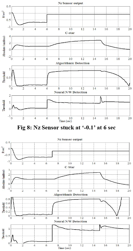
In order to detect stuck sensor fault, offline signal processing was carried out to identify signatures of fault for the aircraft in the collected data. This step is called feature extraction and is one of the most important steps in building a successful diagnostic system. For a practical implementation, it is desirable that the features be not only computationally inexpensive, but also explainable in physical terms. They should be fairly insensitive to external variables like noise and uncorrelated with other features. Keeping these criteria in mind, a set of four features was selected (C-Star value, Nz sensor output, q sensor output and input elevator command) that were expected to detect fault and distinguish a healthy system. Out of these four features, C-Star value was the most dominant one. C-Star values for various stuck fault cases are provided in table 1 to establish the correlation. It can be seen that C-Star values goes on decreasing for the cases where stuck fault approaches steady state value, thus making it difficult to detect stuck fault near steady state.
Matlab program was written to create a neural network with one hidden layer, one input layer and one output layer. Networks are sensitive to the number of neurons in their hidden layers. Too few neurons can lead to underfitting. Too many neurons can contribute to overfitting with poor generalization. Generalization means that neural network should be capable enough to perform correctly for unseen data which was not present in training data. Experimenting with different number of neurons in hidden layers, it was found that nine neurons in hidden layer are giving best performance. Input layer has four inputs which are basically the features extracted from the model. Output layer has one node which will indicate fault. The neural network used is ‘newff’ and the network training function used is “traingd” in MATLAB Neural Network Toolbox [19]. The training algorithm used is Gradient descent backpropagation algorithm (traingd). MATLAB network training function “traingd” updates weight and bias values according to gradient descent. The weights and biases are updated in the direction of the negative gradient of the performance function.
Back propagation training algorithm works on training data so that the cycle error is lesser than the minimum error allowed. The error signal vector is determined in the output layer first and then it is propagated back toward the network input nodes. The training data is created by introducing fault in the model at only one time instants and seven fault values. The neural network is taught with that training data. The final updated or learned neural network is used to generate neural network model, as shown in Fig3, using “gensim” function of MATLAB. Sampling period of neural network is kept as
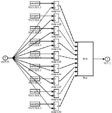
[image:4.595.66.252.77.205.2]20ms which is same as other blocks used for simulationinFig 5. This means that neural network will be giving its output for every 20ms. In Fig 3, x{1} behaves as input layer with 4 nodes, Layer 1 is hidden layer and Layer 2 is output layer. Hidden layer consists of 9 neurons and its detailed simulation diagram is shown in Fig 4 which was generated in MATLAB Simulink.
Fig 3: Neural network model generated by Simulink
Fig 4: Simulink model of Hidden layer of 9 neurons
4.
Simulation Set-up and Fault Induction
Simulation has been carried out for sensor fault detection for F8 aircraft model using Simulink tool [20]. The output of aircraft short period dynamic model consists of Nz and q as shown in Fig 5. Fault is introduced in the Nz sensor of the aircraft model which will be successfully detected by two methods, namely Algorithmic and KBNNFD method. Fault induction is done with the help of N-sample switch [20] as shown in Fig 5. Stuck fault of ‘-0.2’ is induced at 8 sec in the model as one of the fault cases. It is explained with if-else statement and later as Simulink block.
[image:4.595.322.542.248.470.2]Fig5: Simulink model for sensor fault detection
5.
Discussion of results
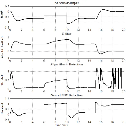
Output consists of Nz sensor and q sensor as discussed in section 2. Fault considered for simulation study is Nz sensor fault. Sensor can fail at any point of time. Stuck fault is considered where sensor gets stuck at one position and erroneously gives aconstant output. This output is the last value of the sensor at the time instant when it failed. Stuck fault are introducedat various time instants for Nz sensor. Fig 6 shows the graph for healthy model. Pitch up command for elevator is given to the model as step input along with noise which has uniform distribution. All the four features extracted for KBNNFD are shown for healthy stable scenario in Fig 6. The model generates the steady value of ‘-0.67ft/s2’ for Nz sensor output. The C-Star value for healthy model is approximately ‘1’ which becomes ‘0’ when the input returns to zero.
It is assumed that while moving from 0 to steady state value of ‘-0.67’, the Nz sensor can get stuck at any value. As fault occurs, all the four features are affected with C-Starbeing the most dominant one. C-Starvalue can go up to 3 for faulty cases. Various cases of stuck fault at values ranging from ‘0’ to ‘-0.55’ are considered and detection is shown using two methods (Algorithmic method and KBNNFD technique.)
Algorithmic technique compares the output from observer and plant. When the difference between the two goes beyond a limit, fault is detected and declared.Based on simulation, threshold value of 0.8 has been arrived at to avoid false alarm.Threshold value is same for both thefault detection technique.
The system is under continuous observation and fault monitoring done every 20ms.Ifthe fault disappears, theoutput of the fault indicator will be less than the threshold value.Furthermore, it is important that the output of the fault indicator is above the threshold till the fault is cleared.Each figure is showing Nz sensor output of the aircraft model which also shows where the fault is introduced. Figures (7 to 15)and table 1 include C-Starvalue as that is most dominant feature used in KBNNFD. All the results are summarized in table 1 with their corresponding figures.
It can be seen in table 1 that for up to -0.4 stuck faults, KBNNFD took one sampling period of 20ms to detect fault. However,it is taking 0.56 sec to detect stuck fault of ‘-0.3’ in transient state. More time is required to detect faultas the stuck value is approaching steady state. Trained neural network used in KBNNFD detects fault at any value of time, t and for any stuck value up to ‘-0.55ft/sec2’.
Table 1:Comparative performance of Algorithmic and KBNNFD technique for detection of stuck sensor fault for Nz sensor. S.
No
Stuck fault value, Nz
(ft/sec2)
C-Star maximum
value (Unit less)
Fault Induction time (sec)
Fault detected time KBNNFD (Neural N/W Detection)(sec)
Fault detected
time Algorithmic
(sec)
Time taken to detect
fault KBNNFD
(sec)
Time taken to detect
fault Algorithmic
(sec)
Corresponding Figure providing all
details
1 0 3.1 5 5.02 5.13 0.02 0.13 Fig 7
2 -0.1 2.76 6 6.02 6.5 0.02 0.5 Fig 8
3 -0.2 2.43 7 7.02 13 0.02 5.0 Fig 9
4 -0.35 2.01 6 6.02 Not detected 0.02 - Fig 10
5 -0.45 1.71 6 6.6 Not detected 0.6 - Fig 11
6 -0.5 1.56 6 7.76 Not detected 1.76 - Fig 12
7 -0.55 1.39 8 13.44 Not detected 5.44 - Fig 13
8 -0.3 2.2 0.5 1.06 Not detected 0.56 - Fig 14
(Transition)
9 -0.4 1.67 6 to 10 6.02 to 10.02 Not detected 0.02 - Fig 15
[image:5.595.52.548.586.761.2]Stuck fault of Nz sensor at ‘-0.1’ was detected by KBNNFD technique in 20ms while algorithmic method took 6.5s. This becomes very critical in scenario during theflight maneuvers. As KBNNFD method does not depend on any observer output to calculate error between the plant model and observer model, there is no ground for error due to observer model imperfections.
To summarize KBNNFD is better in the following ways:
Fault near steady state can also be detected.
Faster detection in KBNNFD for all stuck fault cases.
Model imperfections are taken care by KBNNFD.
[image:6.595.317.540.71.492.2] Detection of Intermittent stuck faults
[image:6.595.57.280.171.439.2]Fig 6: Healthy Model: 4 features of KBNNFD
Fig 7: Nz Sensor stuck at ‘0’ at 5 sec
Fig 8: Nz Sensor stuck at ‘-0.1’ at 6 sec
Fig 9: Nz Sensor stuck at ‘-0.2’ at 7 sec
6.
Conclusion
[image:6.595.57.281.186.674.2] [image:6.595.60.280.446.681.2]better than algorithmic method as it took lesser time to detect the fault in the same condition. KBNNFD technique could also detect the fault near steady state which was not possible with algorithmic method based detection.KBNNFDtechnique was generalized enough to successfully detect fault for all the possible cases of Nz stuck up to ‘-0.55 ft/s2’. KBNNFD successfully detected fault with an imperfect model of aircraft. Non-linearities are considered similar to imperfect models, where the model parameters (elements of A,B,C,D matrices of eqn. 3) are randomly altered. Normal distribution is followed in changing the values randomly by ±10% from their nominal values. The repetition of Simulink experiments indicated that KBNNFD is still valid.Fault cases where Nz sensor is stuck at random values and becomes healthy intermittently were also detected by KBNNFD.In addition to above improvements, neural network is inherently capable of handling nonlinear dynamic system without any approximation.
[image:7.595.307.533.66.741.2]This work can be extended to train the KBNNFD to detect failure of either Nz or q sensor.Other neural network techniques need to be studied to come out with best strategy for sensor fault detection. Implementation techniques need to be studied on FPGA or other hardware.
Fig 10: Nz Sensor stuck at ‘-0.35’ at 6 sec
Fig 11: Nz Sensor stuck at ‘-0.45’ at 6 sec
Fig 12: Nz Sensor stuck at ‘-0.5’ at 6 sec
Fig 13: Nz Sensor stuck at ‘-0.55’ at 8 sec
[image:7.595.51.275.323.726.2]Fig 15: Nz Sensor stuck intermittently between 6 to 10 sec at ‘-0.4’
7.
ACKNOWLEDGMENTS
The authors thank the authorities of BMS Institute of Technology,Reva Institute of Technology and Management and The Director, R & D Cell, JNTU, Hyderabad for their encouragements.
8.
REFERENCES
[1] Paul M. Frank, “Fault Diagnosis in Dynamic Systems Using Analytical and Knowledge-based Redundancy” Pergamon Press plc © 1990 International Federation of Automatic Control, Survey Paper
[2] Thomas Kerr, “Decentralized Filtering and Redundancy Management/Failure Detection for Multisensor Integrated Navigation Systems,” IEEE Transactions on Information Theory, 1986, pp.191~208.
[3] T.V. Rama Murthy and V. Seshadri, “An aid of Mechanization of flight control systems on microcomputers”, Defense Science Journal, DESIDOC, Vol 44 no 2, 1994, pp 119-129.
[4] Shapiro E Y, Schenk F L &Decarli H E, “Reconstructed flight control sensor signals via Luenberger observers, IEEE, 1979, AES-155, pp 245-252.
[5] R.C. Montgomery, A.K. Caglayan, “Failure Accommodation in Digital Flight Control Systems by Bayesian Decision Theory” Journal of Guidance and Control, Vol.13, No.2, 1976, pp.69~75.
[6] R.N. Clark, W. Setzer, “Sensor Fault Detection in a System with Random Disturbances”, IEEE Transactions on Aerospace and Electronic Systems, Vol.AES-16, No.4, 1980, pp.468~473.
[7] M.N. Wagdi, “An Adaptive Control Approach to Sensor Failure Detection and Isolation,” Journal of Guidance, Vol.5, No.2, 1982, pp.118~123.
[8] G. Heredia, A. Ollero, M. Bejar and R. Mahtani “Sensor and actuator fault detection in small autonomous helicopters” (2008), Mechatronics, Vol. 18, N.2, pp. 90-99.
[9] Napolitano MR, et al. “Kalman filter and neural network approaches for sensor validation in flight control systems”, IEEE Control Systems Technology 1999; 6(5):596.
[10]Marcello R. Napolitano, Younghwan An, Brad A. Seanor, “A fault tolerant flight control system for sensor and actuator failures using neural networks” Aircraft Design 3, Pergamon, Elsevier, 2000, pp 103-128. [11]Giampiero Campa1, Mario L. Fravolini2, Brad Seanor1,
Marcello R. Napolitano1, Diego Del Gobbo1, Gu Yu1, SrikanthGururajan, “On-line learning neural networks for sensor validation for the flight control system of a B777 research scale model” International Journal of Robust and Nonlinear Control, Special Issue: Applications of Neural Networks in Control and Instrumentation, Volume 12, Issue 11, 2002, pp 987–1007.
[12]Lennon R. Cork, Rodney Walker, Shane Dunn, “Fault Detection, Identification and Accommodation Techniques for Unmanned Airborne Vehicle” Australian International Aerospace Congress, Melbourne, 2005 [13]Judd, K. & Smith, L.A. “Indistinguishable states II The
imperfect model scenario”, Physica D-Nonlinear Phenomena, 196, 2004, pp 224-242.
[14]Levin, A.U., Narendra, K.S. “Control of Non-Linear Dynamical Systems Using Neural Networks: Controllability and Stabilization”, IEEE Transactions on Neural Networks, Vol.4, No.2, 1993, pp.192~206. [15]Hartmann G.L., Hauge J.A. &Hendrick R.C. “F8C
digital CCV flight control laws”, NASA, Washington D.C., 1976. NASA CR-2629
[16]Mooij H. A. “Criteria for low speed longitudinal handling qualities” MartinusNijhoff Publishers, Netherlands, 1984.
[17]Pau, “L.F. Failure analysis and performance monitoring”, Marcel Decker, 1981.
[18]M. Gopal, “Digital Control & State Variable Methods”, Tata McGraw Hill, 2003
[19]Jacek M. Zurada, “Introduction to artificial neural systems”, West, 1992.