Robust PID Controller Design for Non Minimum Phase Systems using Magnitude Optimum and Multiple Integration and Numerical Optimization Methods

(1)

© 2017, IRJET | Impact Factor value: 6.171 | ISO 9001:2008 Certified Journal

| Page 1474

Robust PID Controller Design for Non-Minimum Phase Systems Using

Magnitude Optimum and Multiple Integration and Numerical

Optimization Methods

M. Anil Kumar

1

_{, B. Amarendra Reddy}

2

1

_{PG Student, EEE-Dept. Andhra University, Visakhapatnam, India.}

2

_{Assistant Professor, EEE-Dept. Andhra University, Visakhapatnam, India.}

---*---Abstract -**

In this paper the controller design for non

minimum phase systems are obtained by using magnitude optimum and multiple integration method and numerical optimization approach. There are many ways to design a proper controller for a specific system. This paper mainly focused on the optimization approach methods. In this paper non minimum phase systems are used for design controller.

Key Words:Magnitude optimum and multiple integration

method, Numerical optimization approach, Non minimum phase systems, Controller parameters.

1. INTRODUCTION

There have been great amount of research work on the tuning of PID controllers. In this paper, two approaches are given for the controller design of non minimum phase systems. PID controllers have been used for a long time. Taylor developed the first PID controller. But the problem is occurred in how to tune a PID controller. at that time Ziegler and Nichols discover the famous Ziegler and Nichols tuning rules. These rules are still widely used. This is why so many different tuning rules have been developed which are based on the same tuning procedure. by this way In this paper discussed about the controller design of the non minimum phase systems by using magnitude optimum and multiple integration and numerical optimization approach. Generally a non minimum phase system is meant by among all systems having the same magnitude plot, those with the least phase shift range are called minimum phase. Remaining are all non minimum phase. The transfer function of a MP system can be determined from the magnitude alone. systems having rhp zeros are non minimum phase. but they’re not the only ones. every rational transfer function has a high frequency magnitude asymptote with slope -20(n-m)dB/dec, where n is the number of poles and m is the no of zeros. every rational, minimum phase transfer function has high frequency phase asymptote at-90(n-m).use these facts to detect non minimum phase systems from their bode plot. if a transfer function has poles and /or zeros in the right half plane then the system shows non minimum phase behavior. In this paper find the controller parameters of same non minimum phase system by using magnitude optimum and

multiple integration and numerical optimization approaches by using their controller design process.

2. MAGNITUDE OPTIMUM AND MULTIPLE

INTEGRATION METHOD

ROBUST CONTROLLER DESIGN:

The problems with original MO tuning method just mentioned can be avoided by using the concept of ‘moments’. This can be done by repetitive (multiple) integrating the input (u) this method is called magnitude optimum multiple integration (MOMI) tuning method Derivation of PID controller parameters:

Assume that the rational transfer function of the actual process be:

1 2 1 2

2 2

1 ....

( ) ;

1 ....

del

m sT m

P PR n

n

b s b s b s

G s K e

a s a s a s



   



    (1)

Here Kpr denotes the process steady-state gain, and

a

₁ to

n

a and b1to bm are the parameters (m



n) of the process

transfer function, and here

T

del represents the process

pure time delay.

The following transfer function is describes the filtered PID controller

:

( ) ( )

( )

C

U s G s

E s

  ki

s



k



1

d

f

sK sT



(2)

Where U and E denotes the Laplace transform of controller output and the controller output, and the controller error (e=w-y), respectively. Here Kiis represented as integral

gain,Kis represented as proportional gain, d K is

represented as derivative gain and Tfis called as filter time

(2)

© 2017, IRJET | Impact Factor value: 6.171 | ISO 9001:2008 Certified Journal

| Page 1475

time delay, by using Taylor series the time delay will transformed into polynomial form.

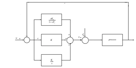
i

K s 1

d f

sK sT



+ +

++

K

-w e _process

d u

[image:2.595.51.283.131.247.2]

a

Fig. 1. The closed loop system with PID controller

The open- loop system transfer function can be given as follows:

1

2 3

0 1 2 3

2 3

0 2 3

....

( ) ( ) ;

....

c P

d d s d s d s

G s G s

c c s c s c s

   



    (3)

Parameters ci and di(i=1,2,…….) can be expressed as

functions of the parameters in the transfer function(1),PID controller(2) parameters, and parameters of Taylor’s expansion:

1 ,

1 2

[ ( ) ( ) ],

i i i f

i pr i i i f i f d i

c a a T

d K K  K T K  KT K 



 

 

     (4)

Where

0

0 0

( 1)

,

(

)!

1,

0,

0.

i k i

i k del

i

k k

i i

T

b

i

k

a

b

a

b

i



 







 





(5)

Let us first assume that filter time constant (T_f) is given. in

order to determine three control parameters (K K K_i_, , _d),as

required by the given magnitude optimum criterion, the first three equations(

n

 

0

2

) from the following set of equations(Hanus,1975)must hold:

2 1 2

0 0

1

( 1) ( 1) .

2

n n

i i

i n i i n i

i i

d c c c



  

 

  



(6)

To calculate the parameters K K_i, ,andK_d of the controller,

the expression (4) into (6) then applying n=0,1,and2. Then the result occurred is

1( , 1, 2,...., 5, 1, 2,...., 5, del, ),

i pr f

K  f K a a a b b b T T (7)

1

2( pr, 1, 2,...., 5, , 2,...., 5, del, f),

K f K a a a b b b T T (8)

1

3( , 1, 2,...., 5, , 2,...., 5, del, ).

d pr f

K  f K a a a b b b T T (9)

Hanes (1975) was defined the necessary stability condition as

0 0

0. d c 

The above inequality verifies that the nyquist curve starts (at



=0) bellow the real axis (

I

m< 0).

The control parameters are depends on 12 process parameters from (7) to (9). The accurate estimation of the 12 parameters from real measurements could be very problematic. To avoid this problem use the concept of repetitive integration technique. This concept is based on the measurement of areas which are calculated from the process open-loop step response. The areas Ai (i=0,1,….) can be

expressed by integrating the process input (u(t) and the process output(y(t)) after applying the step change ∆U at the process input:

0 0( ) , ( )

pr

k k

A y K

A y

  

 

1

(( 1) ( ) ( 1) )

!

i k

k k i del k i

pr k k

i

T b

K a b

i

  



  



 + 1 1

1

( 1) ,

k

k i i k i i

A a

  

 





(10) Integrals are defined as follows:

0

( ) (0) ( ) y t y , y t

U

 



1 1

0

( ) [ ( )] .

t

k k k

y t 



A y  d (11)

By using the expression (10) the all areas are coming Using the expression (10) it is possible to eliminate all the 12 process parameters from (7)-(9).he controller parameters

i

K ,K and, K_d are:

2 2 3

2 3 1 4 ( 2 0 4) 1 2 0 2

2

f f f

i

A A A A T A A A T A A T A A

K      



(12)

2 2 3

3 1 5 ( 2 3 0 5) 1 3 0 3

2

f f f

A A A T A A A A T A A T A A

K     

 (13)

3 4 2 5

, 2

d

A A A A

K  

 (14)

(3)

© 2017, IRJET | Impact Factor value: 6.171 | ISO 9001:2008 Certified Journal

| Page 1476

2 2

1 2 3 0 1 5 1 4 0 3

2 2

1 2 0 5 0 1 4 0 2 3

2 2 3 2

1 2 0 1 3 0 1 2 0 3

( )

( ) ( ).

f

f f

A A A A A A A A A A T A A A A A A A A A A T A A A A A T A A A A A

    

   

   

(15)

The above expression can be write as:

i

d

K K K

 

 _{ }

 

 

1

1 0

3 2 1 0

2 3

5 4 3 1 0

0 0.5

0 0

f f f

A A

A A A T A

A A A T A T A



   

_ _{ }  __ _

   

_    _ _ _

 

(16)

By using this expression controller parameters K K andKi, , d

are calculated.

3. NUMERICAL OPTIMIZATION APPROACH

Numerical optimization presents a comprehensive and up to date description of the most effective methods in continuous optimization it responds to the going inters in the optimization engineering. In this paper design the controller for a no minimum phase system using numerical optimization method.

Due to its simplicity, robustness and wide ranges of applicability in the regulatory control layer, the (PID) controller is use widely. However, a very broad class is characterized by a periodic response. The commonly used category of industrial systems can be represented by a first-order plus dead time model given as,

0

( )

1

t s

ke

G s

s









(17)

For the purpose of simplified analysis, this process model can only be used.. But the actual may have multiple lags, non-minimum phase zero, etc. Similarly, another industrial process is characterized as non-a periodic response. This is represented by a second-order plus dead-time model given as,

0 2

1 0

( )

t s

ke

G s

s

a s

a







(18)

Robust PI/PID Controller design

Assume classical and very well known feedback control system show in figure, here G(s) represents the transfer function model and K(s) is the transfer function of standard PI/PID controller

Σ

  



R(S)

U(S) E(S) _K(S)

D(S)

G(S)

[image:3.595.39.273.188.233.2]

Y(S)

Fig. 2. PID feedback control system

PID: ( ) i

p d

k K s k k s

s

  

(19)

The transfer function of the closed loop system is respectively defined as Sensitivity Function S(s)

1 1

( )

1 ( ) ( ) 1 ( )

S s

K s G s L s

 

  (20)

Where, L S

 

K s G S

   

is the open-loop transfer function,

and Complementary sensitivity function C(S)

( ) ( ) 1 ( )

1 ( ) L s C s S s

L s

  



(21)

SECOND ORDER PID CONTROLLER DERIVATION

The open loop transfer function of standard PID controller is

0

2 0 2

1 0

(1 )(1 )

( )

t s p i d i

i

k k T s k T s P s e

L s

T s s a s a



  



  , with Ti1ki. And using

the approximation 0

0

1 (1 )

t s

e

t s

 _

 .

Now the open loop transfer function is given by

0

2 0 2

1 0

(1 )(1 )

( )

t s p i d i

i

L s

T s s a s a



  



 

Now the closed loop transfer function is given by

0

2 0 2

1 0

2 0 2

1 0

(1 )(1 )

( ) ( )

(1 )(1 )

1 ( )

1

( )

t s p i d i

i

t s p i d i

i

L s T s s a s a

L s

T s s a s a



  

 



  



  (22)

Therefore, the polynomial characteristic equation f the closed loop system is given by

1 0 0 0

4 3 1 0 0 2

0 0

1

( ) ( )

d p d

p i

i i

a a t kk kk P

a t kk P

s s s

t t

kk T kP a k

s s

T t T t 

  

 

  

 

 

Which is in the form of 2 2

0 0

( )

s

(

s

a s

)(

2 s

)

(4)

© 2017, IRJET | Impact Factor value: 6.171 | ISO 9001:2008 Certified Journal

| Page 1477

4 3 2 2 2

0 0 0

2 2 2 2

0 0 0

( ) (2 2 ) ( 4 )

(2 2 )

s s s a s a a

s a a a















     

   (23)

By comparing (21) and (22) we get

0

1 0

0 0

1 1

2 2 2

d

kk P a a

t t 

   

2 2

0 0 0 0 0 0 0

(2( ) )

p

a a t a P t a

k

     



2 2

0 0

i

a t

k k





1 0 0 0 0

0

1 2 2

d

a t t at

k

kP



  



The closed-loop stability impose a > 0 which is verified if

0 1

0 0 0

1 1 1

( ) 1

2 2 2

d

kk P a

t t

   

The above inequality is satisfied for

0 1

0 0 0

1 1 1

( )

2 2 2

d

kk P

a b

t t

   

With b > 1. Taking into account the first constraint one can choose

 



m which gives

0

0 1

0 0

1 1 1

( )

2 2 2

d

m

kk P a

b t t

 

  

0

1 0

0 0

1 1

2 2 2

d m

kk P a a

t t  

   

Therefore, the optimization problem is then written as

0

1

2 0 2

1 0 0

0 1

0 0

0

1 0

0 0

2 2 0 0 0 0 0 0 0 2 2

0 0

1 0 0 0 0

0

max {min 1 ( , ) }

(1 )(1 )

( )

1 1 1

( )

2 2 2

1 1

2 2 2

(2( ) )

1 2 2

b

t s

p i d i

i

d

m

d m

m p

i

m d

L j b

k k T s k T s P s e L s

T s s a s a kk P a

b t t

kk P a a

t t

a a t a P t a k

k a t

k k

a t t at k

kP

 

 

 

   



  

 

  



 

  

   

  



  



(24)

4. EXAMPLES.

To show the effectiveness of these PID controller design methods for non minimum phase systems are considered for simulation in MATLAB.

Example 1:

Case (a) : magnitude optimum and multiple integration method:

Consider the second-order system described using a transfer function G s₁( ). The PID controller parameters are

obtained using magnitude optimum multiple integration method the detailed step-by step computation procedure is given as below.

1 2

(1 3 ) ( )

2 1

s

s e G S

s s



 

 

Here in this problem areas which are obtained from the expression (10) is:

0 1 2 3

4 5

1, 1,

1, 6, 14.50000, 21.6667 29.2083, 36.8833

pr del

K T

A A A A

A A

 

   

 

0.01

f

T 

By substituting these values of areas in expression (16) the parameters values are obtained as

0.1186, 0.2114, 0.0826

i p d

K  K  K 

Case(b):

Numerical optimization method:

1 2

(1 3 ) ( )

2 1

s

s e G S

s s



 

 

From the expressions (24) in The controller parameters are:

0 1 0 0

0

1; 2; 3; 1; 1;

0.5; 3; 0.75; 0.7500

0.2188; 0.1406; 0.2500

p i d

a a p t k

b a

K K K

 

     

   

(5)

| Page 1478

0 10 20 30 40 50 60 70 80 90 100

-1 -0.5 0 0.5 1 1.5

Step Response Comparison of (1-3s)exp(-s)/(s2+2s+1)

Time response

y

MOMI NA

Fig.3. Time response of with MOMI and NA controllers

Example 2:

Case (a): magnitude optimum and multiple integration method:

Consider the second-order system described using a transfer function G s2( ). The PID controller parameters are

obtained using magnitude optimum multiple integration method the detailed step-by step computation procedure is given as below

.

0.2

2 2

1.5( 0.2 1) ( )

2 1

s

s e

G s

s s



 



 

0 1 2 3

4 5

1.5, 0.2,

1.5, 3.6, 5.75, 8.0 10.19, 12.4

pr del

K T

A A A A

A A

 

   

 

0.01

f

T 

0.8081, 1.6060, 0.7894

i p d

K  K  K 

Case (b):

0.2

2 2

1.5( 0.2 1) ( )

2 1

s

s e G s

s s



 



 

From the expressions (24) The controller parameters are:

0 1 0 0

0

1; 2; 0.2; 0.2; 1.5;

0.9; 4.6; 0.75; 2.2325

0.8203; 0.5383; 0.7900

p i d

a a p t k

b a

K K K

 

    

   

  

0 10 20 30 40 50 60 70 80 90 100

-0.5 0 0.5 1 1.5

Step Response Comparison1.5(1-0.2s)exp(-0.2s)/(s2+2s+1)

Time response

y _MOMI

NA OPT

Fig.4. Time response with MOMI and NA

controllers

Example 3:

Case (a) : magnitude optimum and multiple integration method:

0.2

3 2

(1 4 )

( )

3

2

s

s e

G S

s







0 1 2 3

4 5

1, 0.2,

1, 7.200, 21.4200, 56.983 149.5291, 391.6061

pr del

K T

A A A A

A A

 

   

 

0.01

f

T 

0.1180,

0.3496,

0.1061

i p d

K



K



K



Case(b):

0.2

3 2

(1 4 )

( )

3

2

s

s e

G S

s







From the expressions (24) in The controller parameters are:

0 1 0 0

0

2; 3; 4; 0.2; 1; 0.5; 7.5; 0.75; 2.4375

0.232; 0.2971; 0.1188

p i d

a a p t k

b a

K K K

 

    

   

(6)

| Page 1479

0 20 40 60 80 100 120 140 160

-1 -0.5 0 0.5 1

1.5 Step Response Comparison Of (1-4s)exp(-0.2s)/s

2_+3s+2

Time response

y MOMI

NA

Fig.5. Time response with MOMI and NA controllers

CONCLUSION.

This paper deals with the two approaches for controller design for PID controllers. Which are obtained by MOMI and Numerical optimization approaches. It is observed that MOMI method is giving accurate results when compared with Numerical optimization method. second order systems are considered for simulation in mat lab.

REFERENCES

(1) Vrančić, D. (2008). MOMI Tuning Method for Integral Processes. Proceedings of the 8Th_{Portuguese Conference on}

Automatic Control, Vila Real,

(2) Astrom, K. J., Panagopoulos, H. & Hagglund, T. (1998). Design of PI Controllers based on Non-Convex Optimization. Automatic, 34 (5), pp. 585-601.

(3) Ba Hli, F. (1954). A General Method for Time Domain Network Synthesis. IRE Transactions– Circuit Theory, 1 (3), pp. 21-28.

(4) Gorez, R. (1997). A survey of PID auto-tuning methods. Journal A. Vol. 38, No. 1, pp. 3-10.

(5) Hanus, R. (1975). Determination of controllers parameters in the frequency domain. Journal A, XVI (3).

(6) Huba, M. (2006). Constrained pole assignment control. Current Trends in Nonlinear Systems and Control, L. Menini, L. Zaccarian, Ch. T. Abdullah, Edts., Boston: Birkhauser, pp. 163-183

.

(7) Kessler, C. (1955). Uber die Vorausberechnung optimal abgestimmter Regelkreise Teil III.Die optimale Einstellung des Reglers nachdemBetragsoptimum.Regelungstechnik, Jahrg. 3, pp. 40-49.

(8) Preuss, H. P. (1991). Model-free PID-controller design by means of the method of gain optimum (in German). Automatisierungstechnik, Vol. 39, pp. 1522.

(9) Rake, H. (1987). Identification: Transient- and frequency-response methods. In M. G. Singh(Ed.), Systems & control encyclopedia; Theory, technology, applications. Oxford:Pergamon Press.

(10) Strejc, V. (1960). Auswertung der dynamischen Eigenschaften von Regelstrecken bei gemessenen Ein- und Ausgangssignalen allgemeiner Art. Z. Messen, Steuern, Regeln, 3(1), pp. 7-10

Robust PID Controller Design for Non Minimum Phase Systems using Magnitude Optimum and Multiple Integration and Numerical Optimization Methods

© 2017, IRJET | Impact Factor value: 6.171 | ISO 9001:2008 Certified Journal

| Page 1474