Generalization of the Global Error Minimization for Constructing Analytical Solutions to Nonlinear Evolution Equations

(1)

http://dx.doi.org/10.4236/jamp.2015.39142

Generalization of the Global Error

Minimization for Constructing Analytical

Solutions to Nonlinear Evolution Equations

Serge Bruno Yamgoué, Bonaventure Nana

Department of Physics, Higher Teacher Training College-Bambili, The University of Bamenda, Bamenda, Cameroon

Email: [email protected], [email protected]

Received 17 August 2015; accepted 15 September 2015; published 18 September 2015

This work is licensed under the Creative Commons Attribution International License (CC BY). http://creativecommons.org/licenses/by/4.0/

Abstract

The global error minimization is a variational method for obtaining approximate analytical solu-tions to nonlinear oscillator equasolu-tions which works as follows. Given an ordinary differential equ-ation, a trial solution containing unknowns is selected. The method then converts the problem to an equivalent minimization problem by averaging the squared residual of the differential equa-tion for the selected trial soluequa-tion. Clearly, the method fails if the integral which defines the aver-age is undefined or infinite for the selected trial. This is precisely the case for such non-periodic solutions as heteroclinic (front or kink) and some homoclinic (dark-solitons) solutions. Based on the fact that these types of solutions have vanishing velocity at infinity, we propose to remedy to this shortcoming of the method by averaging the product of the residual and the derivative of the trial solution. In this way, the method can apply for the approximation of all relevant type of solu-tions of nonlinear evolution equasolu-tions. The approach is simple, straightforward and accurate as its original formulation. Its effectiveness is demonstrated using a Helmholtz-Duffing oscillator.

Keywords

Global Error, Minimization, Heteroclinic Solution, Homoclinic Solution, Front/Kink, Dark/Anti-Dark Soliton

1. Introduction

(2)

ma-thematics, physics and engineering sciences. Among these NEEs, ordinary differential equations (ODEs) de-serve a special attention. In effect, techniques originally developed for solving ODEs are usually applicable to many other types of NEEs by means of appropriate transformations. For instance, partial differential equations (PDE) are commonly turned into ODEs by using the uniform traveling wave transformation [1]. A variant of it, called fractional complex transformation [2] has recently been introduced and enables to transform fractional ODEs into ordinary (i.e., non-fractional) ones. Solving ODEs is therefore an important step for solving NEEs in general.

The solutions of a given ODE can be divided into two groups. The first group comprises unbounded solutions which are of little interest from the viewpoint of applications. The second group is formed of all bounded solu-tions. It may be further divided into three classes: constant solutions also called fixed points or equilibrium points, periodic (including quasi-periodic) solutions, and bounded non-periodic solutions. Constant solutions are usually considered as trivial solutions and are less interesting than the other two classes of solutions. The bounded non-periodic solutions are constituted mainly of heteroclinic and homoclinic solutions. They are solu-tions with the specific property of being backward and forward asymptotic to two distinct or the same fixed points (see (4), (5) and (6) below), respectively. In the case of ODEs resulting from wave equations through the uniform travelling wave transformation, they are called soliton and are the most important for the corresponding field of applications.

While exact and closed-form analytical expressions for the solutions of interest are the eventual targets of the continuing research work, it has long been recognized that such solutions are in general impossible, or at best very difficult to obtain. Thus, the efforts dedicated to constructing analytical solutions to nonlinear ODEs are dominated by the development of approximate methods, that is, methods leading to approximate analytical solu-tions. Numerous approximate analytical techniques are now available in the literature as the results of these ef-forts. They include: the Newton harmonic balance [3]-[8], the linear-delta expansion [9], the Homotopy analysis method [10], the method of cubication [11]-[13], the rational harmonic balance method [14], the global error minimization [15], the recent method of quintication [16], to name just a few. Although some of these tech-niques are very competitive with respect to accuracy, rate of convergence and ease of use, there is always a room for some improvements.

We observe for instance that in the expositions as well as the subsequent applications of all the techniques mentioned above, only periodic motions and their periods are concerned. In fact, a search through the relevant literature indicates, to the best of our knowledge, that most of the approximate methods published so far are de-signed to deal only with periodic solutions. Non-periodic solutions such as heteroclinic or homoclinic solutions are largely neglected in spite of their well-recognized importance for wave propagation. The development of methods that are also applicable to these types of solutions is undoubtedly desirable. This is our purpose in this paper where this task is tackled through the generalization of an existing method, namely the global error mini-mization.

The organization of this paper is as follows. In the next section, we revisit the global error minimization me-thod and generalize so as to make it applicable both to periodic and bounded non-periodic solutions. In Section 3, we illustrate the proposed generalization by applying it to the determination of non-periodic solutions of an ODE. We end with our conclusions in Section 4.

2. Revisiting the Global Error Minimization

In this section, the global error minimization [15] for constructing analytical solutions to ODEs is briefly revi-sited. For the sake of clarity of the presentation, we consider a general second order ODE of the

(

, ,

)

0

x+F x x t =

  (1)

which governs the time (t) evolution of the state (x) of a conservative single degree-of-freedom system. Here, an overdot denotes differentiation with respect to time t. Thus, x=x t

( )

is a real scalar function. In general, (1) is supplemented with initial conditions of the form

( )

0 ,

( )

0

x =A x =B (2)

where A, B are real constants. Depending on the combination values of these constants and on the function

(

, ,

)

(3)

approximations to periodic solutions of (1) with (2) can be obtained as functions satisfying (2) which minimize the functional

( )

(

)

0

2π

, , , d , ;

T

E x t = x+F x x t t T=

Ω

∫

  (3)

where Ω is the unknown angular pulsation of the approximated periodic solution and the “norm” here is de-fined by u =u2. This is the principle of the global error minimization. See [15] for the details.

For bounded non-periodic motions, the integration range in (3) should obviously be modified to cover the whole real domain, i.e., it should span from −∞ to +∞. Now, as pointed out in the introduction, heteroclinic or homoclinic orbits are backward and forward asymptotic to fixed points. In other words, they verify the boun-dary conditions

( )

lim p, lim m, lim 0

t→+∞x t =X t→−∞x t =X t→±∞x t = (4)

with

(

p, 0,

)

(

m, 0,

)

0; x

(

p, 0,

)

0; x

(

m, 0,

)

0.

F X t =F X t = ∂ F X t < ∂ F X t < (5)

The symbol ∂_x means partial derivative with respect to x, the first argument of F. Equation (5) is the simplest case of non-degenerate fixed points. It may be replaced for a degenerate fixed point X_D by

(

)

2 1

(

)

, 0, 0, 1 2 ; , 0, 0

k n

xF XD t k n x F XD t

+

∂ = < ≤ ∂ < (6)

for some positive integer n. If either of X_p or X_m is different from zero, which is the case for all heteroclinic orbits (characterized by X_p≠X_m) and some homoclinic solutions (characterized by X_p =X_m) with X_p≠0, the integral in (3) will not be finite. This means that the above formulation of the global error minimization cannot be applied to these types of solution which, in the context of wave propagation, correspond respectively to kink (or front) wave or dark solitons. To remedy this situation, we propose to replace the functional (3) by

( )

max

(

)

min

ˆ , , , d .

t

E x t =

∫

x+F x x t x t (7)

In this new formulation where the integrand is essentially the product of the original integrand by the velocity, one has to use

(

t_min,t_max

)

=

(

0, 2πΩ

)

for periodic solutions and

(

t_min,t_max

)

= −∞ +∞

(

,

)

for heteroclinic orho-moclinic solutions; with a generalized definition of Ω as a pseudo-frequency in this last case. Here

ˆ x

x

ϑ = 

 (8)

where ϑ comprises all unknowns of the problem appearing in x and such that their vanishings induce the vanishing of the velocity. It can be observed that for velocity-free and time-free restoring force functions, that is,

(

, ,

)

( )

F x x t ≡F x , the integrand of (7) is directly proportional to the time derivative of the total energy of the system,

( )

0

2

, d ;

2

x

x x

H x x =  +

∫

F ξ ξ (9)

which is a constant of motion. However, since it is not the energy itself which is minimized but its time deriva-tive, the present method is different from energy minimization methods available in the literature [17] [18].

An important point in methods of minimization is the determination of the trial function. The quality of the approximation depends crucially on how good the trial solution captures the properties of the exact solution. For periodic solutions of angular pulsation Ω, a theorem due to Fourier guarantees that they admit an expansion of the form

( )

0

(

)

(

)

1

cos sin .

k k

k

x t C C k t S k t

∞

=

= +

∑

Ω + Ω (10)

(4)

monic decreases exponentially as k increases. If the problem additionally possesses the odd-parity property, then its solutions contain only odd harmonics [19]. The information enables to construct good approximations to the periodic solutions by truncating the expansion in (10) to some finite order and eventually retaining only the ap-propriate harmonics.

Contrarily to the case of periodic solutions, little is known on how to construct good approximate trial for non-periodic solutions. Here we propose the following ansatze [20]

( )

1 1

sech k tanh sech j

ho p k j

k j

x t X P t t Q t

∞ ∞

= =

= +

∑

Ω + Ω

∑

Ω (11)

and

( )

1

1 sech tanh

2 2

n

p m p m

he n

n

X X X X

x t R t t

∞

=

+ −  

= + _ + Ω _ Ω



∑

 (12)

for solutions of the homoclinic type or heteroclinic type, respectively. In principle, all of the fixed points X_p or X_m, the pseudo-frequency Ω and the coefficients P_k, Q_j and R_n may be taken as unknowns to be de-termined by the procedure. However, it makes sense to ensure that the type of solution of interest is susceptive to exist by verifying that there exist points X_p and X_m which satisfy either (5) or (6). Whenever possible, they should be determined beforehand and hence removed from the minimization variables. For all homoclinic type solutions and some cases of heteroclinic type solutions, the pseudo-frequency Ω can also be calculated beforehand as the square root of the magnitude of the left-hand-side of the first inequality in (5). This means that only the coefficients constitute the unknowns which are to be determined by the approximation analysis.

Each of the summations in (11) and (12) must obviously be truncated conveniently to keep the analysis ma-nageable, as it is the case when one deals with periodic solutions. Very often, the nonlinear function F in (1) is polynomial. In this case, we suggest the principle of homogeneous balance [20] as a first hand rule for deter-mining the truncation orders, i.e. the highest degrees K_max, J_max and N_max to retain in the respective sums of (11) and (12). According to this principle, K_max, for example, is obtained by requiring that on substituting

( )

max

sech Ωt K in the ODE at hand, the linear term with the highest order derivative and the term with the highest degree of nonlinearity balance each other.

3. Illustrative Example

This section is devoted to the illustration of the revisited formulation of the global error minimization presented above. Our focus is the approximation of homoclinic and heteroclinic orbits for which the classical formulation of the method cannot apply. The model problem chosen for this purpose is described by the Helmholtz-Duffing equ-ation given by

2 3

0.

x+ −x

α

x −

β

x =

 (13)

This is an autonomous conservative system for which the restoring force function is the gradient of the po-tential

( )

2 3 4

. 2 3 4

x

V x = −

α

x −

β

x (14)

When the two coefficients

α

and β are such that 0<

α

2+4

β

as we assume here, (13) possesses three equilibrium points including the trivial stable one x₀=0.The expressions of the two others are

2

4 2

u

x α β α

β

+ −

= (15a)

and 2 4 . 2 u

x α β α

β

+ +

= −

 (15b)

(5)

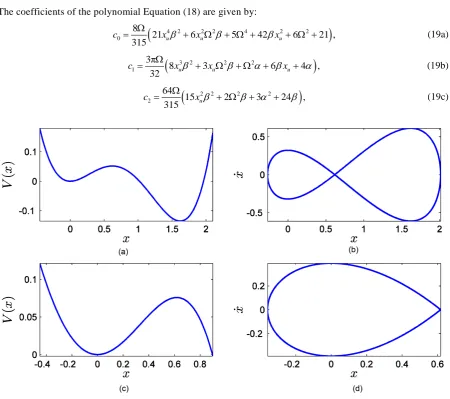
maximum of the potential (14). This maximum is connected to itself in the first case by two homoclinic orbits; and in the second case by one. See Figure 1 for the profiles of the potential and the associated separatrixes.

We now embark on approximating the homoclinic orbits identified above using the generalized formula-tion of the global error minimizaformula-tion proposed in this paper. We shall restrict ourselves to soluformula-tions which contain only the sech function. By applying the principle of homogeneous balance, we determine the trunca-tion order to be K_max=1. The approximate solution is then expressed as

( )

1sech

( )

ho u

x t =x +P Ωt (16)

with

2 2

4 4

. 2

α

β α α

β

+ − +

Ω = (17)

The sole unknown here is P₁. We substitute (16) into the left hand side of (13) and multiply it by

( )

ˆ _tanh _sech

x= − Ωt Ωt . The outcome is squared, and then integrated over the real domain according to (7) to obtain the averaged square residual. By minimizing the latter with respect to P₁, we obtain the equation

2 3 4

0 1 1 2 1 3 1 4 1 0.

c +c P+c P +c P +c P = (18)

The coefficients of the polynomial Equation (18) are given by:

(

4 2 2 2 4 2 2

)

0 8

21 6 5 42 6 21 ,

315 u u u

c = Ω x β + x Ω β+ Ω + βx + Ω + (19a)

(

3 2 2 2

)

1 3π

8 3 6 4 ,

32 u u u

c = Ω xβ + xΩβ+ Ωα+ βx + α (19b)

(

2 2 2 2

)

2 64

15 2 3 24 ,

315 u

[image:5.595.89.540.293.692.2]

c = Ω x β + Ω β+ α + β (19c)

Figure 1. Profiles of the potential ((a) and (c)) and the corresponding homoclinic orbits ((b) and (d)) for Equation (13).

(6)

(

)

3 25π

3 ,

64 u

c = βΩ xβ α+ (19d)

2

4

64 . 105

c =

β

Ω (19e)

Equations (18)-(19) can be solved exactly analytically. But, it is more convenient to analyze them using numerical simulations.

First, we choose

α

= 5,

β

= −1. Then, (18)-(19) admit two negative real and two positive real solutions. As pointed out in [15], the value of the averaged square residual can be used to select the most appropriate solutions. In this way, we find that

1 1.36302030152025839

P= (20a)

and

1 0.90267190134849774

P = − (20b)

are the value which approximate, respectively, the right and left homoclinic orbits of Figure 1(b). Next, we take β =1, keeping α = 5. It is then found that Equations (18)-(19) admit only two negative real solu-tions of which

1 0.59375629253419653

P= − (20c)

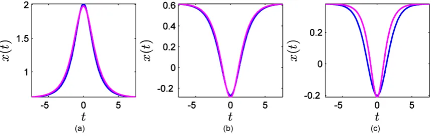
approximates the homoclinic solution of Figure 1(d). We provide a comparison between these approximate solutions to the exact ones in Figure 2. The latter are obtained numerically by using the ode45 function of the Matlab software. One can observe that the accuracy is very satisfactory in spite of the low order of the approximation.

4. Discussion and Conclusions

In this paper, we have proposed a generalization of the method of global error minimization for solving nonli-near ODEs. It consists of establishing the nonlinonli-near algebraic equations verified by the parameters of an ansatz, intended to approximate the solution of a given ODE, by minimizing the averaged product of the derivative of the ansatz with the residual of the ODE for this ansatz. The proposed generalization targets specifically heteroc-linic and non-vanishing tails homocheteroc-linic solutions for which the original formulation of the method could not apply. The non-suitability of the original formulation is due to the fact that the residual alone is generally not square integrable for arbitrary trial solutions. This is also true for other variational methods, including Hamilto-nian and Lagrangian techniques; although the case of homoclinic solutions can be managed by translating the origin to the fixed Xp.

[image:6.595.101.530.550.686.2]

An example has been given to illustrate the effectiveness of the approach. For two different sets of parameters values, we have observed that it yields satisfactory results with, however, varying degree of accuracy; as for all

Figure 2. Comparison of approximate analytical solutions (magenta color) to exact numerical ones (blue color) for the

(7)

approximate methods. Being a variational method, the quality of the results will depend on how good the trial solutions fit the exact ones. We have proposed some general formulae in terms of hyperbolic tangent and secant for constructing such trial solutions for the two specific types of solutions which have been the focus of this work. However other forms, including exponential, algebraic, rational or gaussian can equally be used.

We have concentrated on the case of a scalar variable in our presentation in this paper. But the method can easily be applied to the case of system of coupled ODEs. For, it suffices to consider Xp, Xm, Pk, Qj and

n

R in (11)-(12) as vectors, and then replaces the product of velocity and residual in (7) by the scalar product of their respective vectors. Then, as for trial solutions with several variables, the necessary operations might be-come so tedious that the use of computer algebra systems such as Maple or Mathematica is necessary. In this perspective, an ongoing work is the implementation of the process in such an algebraic manipulator.

References

[1] Griffiths, G.W. and Schiesser, W.E. (2012) Traveling Wave Analysis of Partial Differential Equations: Numerical and Analytical Methods with Matlab and Maple. Academic Press, New York.

[2] Li, Z.B. and He, J.H. (2010) Fractional Complex Transformation for Fractional Differential Equations. Computer and Mathematics with Applications, 15, 970-973.

[3] Wu, B.S. and Li, P.S. (2001) A Method for Obtaining Approximate Analytical Periods for a Class of Nonlinear Oscil-lators. Meccanica, 36, 167-176. http://dx.doi.org/10.1023/A:1013067311749

[4] Wu, B.S. and Lim, C.W. (2004) Large Amplitude Non-Linear Oscillations of a General Conservative System. Interna-tional Journal of Non-Linear Mechanics, 39, 859-870. http://dx.doi.org/10.1016/S0020-7462(03)00071-4

[5] Wu, B.S., Sun, W.P. and Lim, C.W. (2006) An Analytical Technique for a Class of Strongly Non-Linear Oscillators.

International Journal of Non-Linear Mechanics, 41, 766-774. http://dx.doi.org/10.1016/j.ijnonlinmec.2006.01.006 [6] Yamgoué, S.B. and Kofané, T.C. (2008) Linearized Harmonic Balance Based Derivation of the Slow Flow for Some

Class of Autonomous Single Degree of Freedom Oscillators. International Journal of Non-Linear Mechanics, 43, 993- 999. http://dx.doi.org/10.1016/j.ijnonlinmec.2008.05.001

[7] Yamgoué, S.B. (2012) On the Harmonic Balance with Linearization for Asymmetric Single Degree of Freedom Non- Linear Oscillators. Nonlinear Dynamics, 69, 1051-1062. http://dx.doi.org/10.1007/s11071-012-0326-1

[8] Yamgoué, S.B., Nana, B. and Lekeufack, O.T. (2015) Improvement of Harmonic Balance Using Jacobian Elliptic Functions. Journal of Applied Mathematics and Physics, 3, 680-690. http://dx.doi.org/10.4236/jamp.2015.36081 [9] Amore, P. and Aranda, A. (2003) Presenting a New Method for the Solution of Nonlinear Problems. Physics Letters A,

316, 218-225. http://dx.doi.org/10.1016/j.physleta.2003.08.001

[10] Liao, S.J. (2003) Beyond Perturbation: Introduction to Homotopy Analysis Method. Chapman & Hall/CRC Press, Bo-ca Raton. http://dx.doi.org/10.1201/9780203491164

[11] Yuste Bravo, S. (1991) Comments on the Method of Harmonic Balance in Which Jacobian Elliptic Functions Are Used.

Journal of Sound Vibration, 145, 381-390. http://dx.doi.org/10.1016/0022-460X(91)90109-W

[12] Yuste Bravo, S. (1992) “Cubication” of Non-Linear Oscillators Using the Principle of Harmonic Balance. Internation-al JournInternation-al of Non-Linear Mechanics, 27, 347-356. http://dx.doi.org/10.1016/0020-7462(92)90004-Q

[13] Beléndez, A., Méndez, D.I., Fernandez, E., Marini, S. and Pascual, I. (2009) An Approximate Solution to the Duffing- Harmonic Oscillator by a Cubication Method. Physics Letters A, 373, 2805-2809.

http://dx.doi.org/10.1016/j.physleta.2009.05.074

[14] Yamgoué, S.B., Bogning, J.R., Kenfack Jiotsa, A. and Kofané, T.C. (2010) Rational Harmonic Balance-Based Ap-proximate Solutions to Nonlinear Single-Degree-of-Freedom Oscillator Equations. Physica Scripta, 81, Article ID: 035003. http://dx.doi.org/10.1088/0031-8949/81/03/035003

[15] Farzaneh, Y. and Tootoonchi, A.A. (2010) Global Error Minimization Method for Solving Strongly Nonlinear Oscilla-tor Differential Equations. Computers and Mathematics with Applications, 59, 2887-2895.

http://dx.doi.org/10.1016/j.camwa.2010.02.006

[16] Elias-Zuniga, A. (2014) “Quintication” Method to Obtain Approximate Analytical Solutions of Non-Linear Oscillators.

Applied Mathematics and Computations, 243, 849-855. http://dx.doi.org/10.1016/j.amc.2014.05.085

[17] He, J.H. (2002) Preliminary Report on the Energy Balance for Nonlinear Oscillators. Mechanics Research Communi-cations, 29, 107-111. http://dx.doi.org/10.1016/S0093-6413(02)00237-9

(8)

[19] Mickens, R.E. (2002) Fourier Representations for Periodic Solutions of Odd-Parity Systems. Journal of Sound and Vi-bration, 258, 398-401. http://dx.doi.org/10.1006/jsvi.2002.5200