features and BPANN
Praveen N
Research Scholar Department of Electronics Audio and Image Research Laboratory Cochin University of Science and Technology
Kochi, India 682022
Tessamma Thomas
Professor
Department of Electronics Cochin University of Science and Technology
Kochi, India 682022
ABSTRACT
Mel-Frequency Cepstral Coefficients are spectral feature which are widely used for speaker recognition and text dependent speaker recognition systems are the most accurate in voice based authentication systems. In this paper, a text dependent speaker recognition method is developed. MFCCs are computed for a selected sentence. The first 13 MFCCs are considered for each frames of duration 26ms and each coefficient is clustered to a 5 element cluster centres and finally to a form a 65 element speech code vector for the entire speech. The speech code is trained using a multi-layer perceptron backpropagation gradient descent network and the network is tested for various test patterns. The performance is measured using FAR, FRR and EER parameters. The recognition rate achieved is 96.18% for a cluster size of 5 in each coefficient.
General Terms
Speaker Recognition, Artificial Neural Networks, Clustering
Keywords
Mel-Frequency Cepstral Coefficients, False Acceptance Rate, False Rejection Rate, Equal Error Rate
1.
INTRODUCTION
Speaker verification/identification tasks are typically a pattern recognition problem. The important step in speaker recognition is the extraction of relevant features from the speech data that is used to characterize the speakers. There are two speaker dependent voice characteristics: high level and low level attributes [1][2]. Low level attributes related to the physical structure of the vocal tract are categorized as spectral characteristics, whereas high level attributes are prosody (pitch, duration, energy) or behavioral cues like dialect, word usage, conversation patterns, topics of conversation etc. There are two types of speaker recognition methods: text dependent and text independent. Text dependent speaker recognition method uses phoneme context information and hence high recognition accuracy is easily achieved. The text independent speaker recognition method does not require specially designed utterances and hence is user friendly. A general speaker recognition system consists of an enrolment phase and recognition phase.
In the speaker enrolment phase, speech samples are collected from the speakers to train their models. The collection of enrolled models is also called a speaker database. In the
identification phase, a test sample from an unknown speaker is compared against the speaker database. Both phases include the feature extraction step to extract the speaker dependent characteristics from speech..
2.
METHODOLOGY
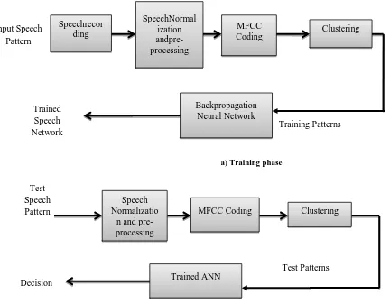
The acoustic analysis based on MFCC has proved good results in speaker recognition. Also MFCC has proved to be good in confrontation with different variation such as noise, prosody, intonation. In this paper, speech samples of a given text are recorded for 40 speakers. 13 MFCCs are computed for about 40-45 frames of voiced speech samples. Vector Quantisation (VQ) based K-means clustering is done for the entire MFCC with respect to the cluster index. The code vector is trained using a discriminative classifier, multilayer perceptron with gradient descent backpropagation ANN. The system is tested with another data set of test patterns. The performance of the system is measured using false acceptance rate (FAR), false rejection rate (FRR) and equal error rate (EER). The result is compared with minimum distance based classifier. The methodology adopted is depicted in fig. 1. In the training phase, speech is recorded and pre-processed. MFC coefficients are computed and clustered using K-means clustering method. The speech code vector thus formed is trained to recognise using backpropagation neural network and stored. In the testing phase, the test speech samples are pre-processed and MFC coefficients are extracted and clustered. The test patterns are given to the trained neural network, which gives a decision of presence or absence of the speech pattern in the database.
3.
FEATURE EXTRACTION
3.1
Speech features
According to Kinnunen [3], a vast number of features have been proposed for speaker recognition, such as:
Spectral features
Dynamic features
Source features
Supra segmental features
High level features
a) Training phase
[image:2.595.37.469.134.471.2] [image:2.595.51.287.545.746.2]b) Testing phase Fig. 1 Speaker Recognition steps
Table 1. Features for speaker recognition Dynamic features relate to time evolution of spectral features. Source features are directly associated with glottal voice source. Supra segmental features span over several segments and high level feature refer to symbolic type of information. Table 1 gives the consolidation of the features for speaker recognition [3]. Since spectral features are the most common and accurate method available [4], a discussion on MFCC based spectral features is followed.
3.2
Speech recording:
In text dependent based speaker recognition, speech samples of the same text/sentence are to be recorded for all the speakers. The speakers are prompted to speak a sentence “open the door”. Speech samples of 40 speakers are recorded in a laboratory environment using a high quality microphone with a DELL T7400 Intel Xeon based workstation computer under MATLAB 7.10.0.1 environment. The speech samples are subjected to the following operations as shown in fig. 1.
Feature Type Examples
Spectral features MFCC, LPCC, LSF, Long-term
average spectrum (LTAS),
Formant frequencies and
bandwidths
Dynamic features Delta features, Modulation
frequencies, Vector
autoregressive coefficients
Source features F0 mean, Glottal Pulse shape
Suprasegmental features F0 contours, Intensity contours,
Micro prosody
High-level features Idiosyncratic word usage,
Pronunciation
MFCC
Coding Clustering
Backpropagation Neural Network Input Speech
Pattern
Trained Speech Network
Training Patterns Speechrecor
ding
SpeechNormal ization andpre-processing
Trained ANN Decision
Test Patterns MFCC Coding
Speech Normalizatio
n and pre-processing
Clustering Test
In order to compensate for the changes in amplitude or energy of the speech recorded at different instances, the samples are normalized pre-processing [5]. Based on the maxima and minima of the signal, normalization has been carried out according to the equation:
𝑥𝑖=1+ 2−1 𝑧𝑖− 𝑧𝑖 𝑚𝑖𝑛
𝑧𝑖𝑚𝑎𝑥 − 𝑧𝑖𝑚𝑖𝑛
1
where xi is the normalized value of zi, and 𝑧𝑖𝑚𝑎𝑥and𝑧𝑖𝑚𝑖𝑛 are
the maximum and minimum values of zi in each sample. 1and2 can be set to 0.1 and 0.9.
3.4
Pre-processing:
As a pre-processing step, pre-emphasis filtering is done for the speech signals. The speech is processed by a
high-dependent information than the lower frequencies. A high pass filter with a transformation
𝐻 𝑧 = 1 − 𝑎𝑧−1 (2)
is used with a=0.95.
3.5
Voiced region extraction:
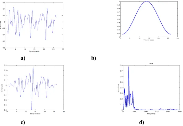
MFCCs of the voiced regions are computed in this work only to minimize the energy due to ambient noise. Hence voiced regions are isolated from the speech signal by considering the energy of the signal. The signal energy is computed and the voiced regions are extracted using the signal energy threshold. The voiced regions extracted for the normalized signal is shown in Fig. 2.
a) b)
c) d)
Fig. 2 a) Speech signal b) Normalized speech signal c) Energy of the signal computed d) Voiced regions extracted
a) b)
c) d)
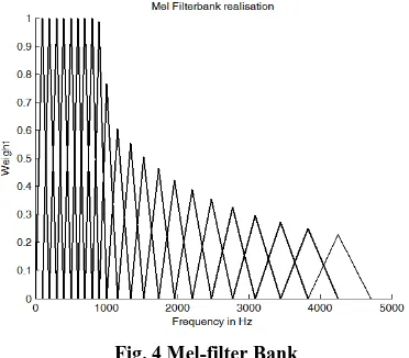
[image:3.595.165.438.260.517.2] [image:3.595.129.421.551.752.2]Fig. 4 Mel-filter Bank
3.6
MFCC Computation:
This method is a short-term spectral analysis method and speech signals are divided into short frames using the popular Hamming window of length 256 points and 256 point DFT is taken (Fig 3). The DFT of the frames is weighted by triangular Mel filterbanks (Fig. 4) and the mel-frequency spectrum at any analysis time 𝑛 is computed as per the equation 4. The next step is to compute the DCT of the log of the magnitude of the filter outputs of each frame, which is the mel-frequency Cepstral coefficient of each frame, as given in equation 3.
𝑚𝑓𝑐𝑐𝑛 𝑚 =1𝑅 𝑅𝑟=1𝑙𝑜𝑔 𝑀𝐹𝑛 𝑟 cos 2𝜋𝑅 𝑟 +12 𝑚 (3)
where
𝑀𝐹𝑛 =𝐴1
𝑟 𝑉𝑟 𝐾 𝑋𝑛 [𝐾]
2 4 𝑈𝑟
𝐾=𝐿𝑟
and 𝐴𝑟= 𝑉𝑈𝐿𝑟𝑟 𝑟[𝐾] 2
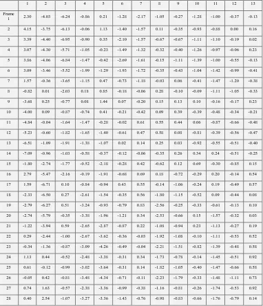
Table 2 shows the MFCC of speech samples computed with
𝑁𝑚𝑓𝑐𝑐 = 13 and R=22.
3.7
Data clustering using K-means method:
The MFCCs are calculated for about 40-45 frames with 13 coefficients for each frames. To reduce the size of the vector used for speaker recognition, clustering of each corresponding coefficients is done with respect to all frames limiting the size of speech vector of each speaker to a 5 × 13 = 65 element vector. k-means clustering, which is a squared mean clustering, is used for this.
The k-Means Algorithm (LBG Algorithm) [6] is as follows:
1. Design a 1-vector codebook which represents the centroid of the entire set of training vectors.
2. Double the size of the codebook by splitting each current codebook yn according to rule
𝐲𝒏+= 𝐲𝒏 1 + 𝜀 𝐲𝒏−= 𝐲𝒏 1 − 𝜀
where n varies from 1 to the current size of the codebook, and is a splitting parameter (e.g.
=0.01)
3. Nearest-Neighbour Search: For each training vector, find the code word in the current codebook that is closest in terms of similarity measurement and assign that vector to the corresponding cell.
4. Centroid update: Update the code word in each cell using the centroid of the training vectors assigned to that cell.
5. Iteration 1: repeat steps 3 and 4 until the average distance falls below a pre-set threshold
6. Iteration 2: repeat steps 2, 3 and 4 until a codebook size of M is designed.
The LBG algorithm designs an M-vector codebook in stages. It starts first by designing 1-vector codebook, then uses a splitting technique on the code words to initialize the search for a 2-vector codebook, and continues the splitting process until the desired M-vector codebook is obtained. In this work, clustering of each of the 13 MFCC’s is done for various cluster sizes ranging from 4 to 10 to find an optimum cluster size which will give the maximum performance during speaker recognition. Clustered speech codebook for cluster size 5 is given in Table 3.
4.
NEURAL NETWORK DESIGN AND
TRAINING
4.1
Network Architecture
Table 2 MFCC of speech samples computed with 𝑵𝒎𝒇𝒄𝒄= 𝟏𝟑 and R=22. (Only 28 frames are shown)
1 2 3 4 5 6 7 8 9 10 11 12 13
Frame
[image:5.595.108.490.183.626.2]1 2.30 -4.03 -6.24 -0.86 0.21 -1.28 -2.17 -1.05 -0.27 -1.28 -1.00 -0.37 -0.13 2 4.15 -3.75 -6.13 -0.06 1.13 -1.40 -1.57 0.11 -0.35 -0.93 -0.88 0.00 0.16 3 3.39 -4.40 -6.95 -0.90 0.35 -2.10 -1.57 -0.67 -0.67 -1.11 -1.10 -0.19 0.02 4 3.07 -4.30 -5.71 -1.05 -0.23 -1.49 -1.32 -0.32 -0.40 -1.26 -0.97 -0.06 0.23 5 3.86 -4.06 -6.84 -1.47 -0.42 -2.69 -1.61 -0.15 -1.11 -1.39 -1.00 -0.55 -0.13 6 3.09 -3.46 -5.52 -1.99 -1.29 -1.93 -1.72 -0.35 -0.43 -1.04 -1.42 -0.99 -0.41 7 1.57 -0.36 -3.65 -1.15 0.47 -0.73 -1.18 -0.03 0.06 -0.41 -1.47 -1.20 -0.38 8 -0.82 0.01 -2.03 0.18 0.85 -0.18 -0.06 0.28 -0.10 -0.09 -1.11 -1.05 -0.33 9 -3.68 0.25 -0.77 0.08 1.44 0.07 -0.20 0.15 0.13 0.10 -0.16 -0.17 0.23 10 -4.00 0.09 -0.87 -0.74 0.41 -0.21 -0.42 0.09 0.39 -0.39 -0.48 -0.34 -0.21 11 -4.84 -0.04 -1.64 -1.47 -0.28 -0.02 0.61 0.55 0.44 0.06 -0.87 -0.66 -0.48 12 -5.23 -0.60 -1.82 -1.65 -1.40 -0.61 0.47 0.58 0.08 -0.81 -0.39 -0.56 -0.47 13 -6.51 -1.09 -1.91 -1.38 -1.07 0.02 0.14 0.25 0.03 -0.92 -0.55 -0.51 -0.40 14 -7.09 -0.96 -1.03 -0.58 -0.37 -0.12 -0.06 -0.35 0.26 0.34 0.24 -0.51 -0.25 15 -1.80 -2.74 -1.77 -0.52 -2.18 -0.28 0.42 -0.62 0.12 0.69 -0.30 -0.85 0.15 16 2.79 -5.47 -2.16 -0.19 -1.91 -0.68 0.69 0.18 -0.72 -0.29 0.20 -0.14 0.54 17 1.59 -6.71 0.10 -0.84 -0.94 0.43 0.55 -0.14 -1.06 -0.24 0.19 -0.49 0.57 18 -2.33 -6.50 0.27 -2.61 -1.54 -0.35 0.56 -1.80 -1.15 -0.52 0.09 -0.44 0.08 19 -2.79 -6.27 0.51 -3.24 -0.93 -0.79 0.83 -2.56 -0.25 -0.33 -0.61 -0.13 0.10 20 -2.74 -5.79 -0.35 -3.38 -1.96 -1.21 0.34 -2.53 -0.66 0.15 -1.57 -0.32 0.03 21 -1.22 -3.94 0.59 -2.65 -2.87 -0.87 0.22 -1.08 -0.94 0.23 -1.13 -0.27 0.19 22 0.29 -2.44 -1.00 -2.67 -3.62 -0.36 -0.03 -1.92 -1.08 -0.10 -1.11 -0.53 0.52 23 -0.34 -1.36 -0.87 -3.09 -4.26 -0.49 -0.04 -2.21 -1.51 -0.82 -1.39 -0.48 0.58 24 1.13 0.44 -0.52 -2.48 -3.38 -0.31 0.34 -1.73 -0.78 -0.14 -1.45 -0.51 0.92 25 0.61 -0.12 -0.99 -3.02 -3.64 -0.31 0.14 -1.82 -1.05 -0.40 -1.47 -0.66 0.58 26 -0.05 0.42 -0.81 -3.48 -4.34 -0.71 -0.11 -2.23 -1.79 -0.33 -1.48 -1.11 0.73 27 0.74 1.63 -0.57 -2.38 -3.36 -0.99 -0.38 -1.16 -0.81 -0.26 -1.74 -0.53 0.92 28 0.40 2.54 -1.07 -3.27 -3.36 -1.43 -0.76 -0.98 -0.83 -0.66 -1.76 -0.79 0.14
Table 3. k-means clustered MFCC of speech samples computed with 5 cluster centers for each coefficient along each column
MFCC’s per frame (13)
1 2 3 4 5 6 7 8 9 10 11 12 13
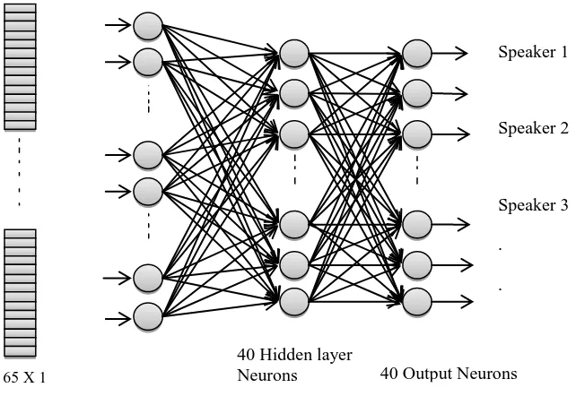
65 X 1 65 Input Neurons
40 Hidden layer
Neurons 40 Output Neurons
Speaker 1
Speaker 2
Speaker 3
.
.
.
.
.
.
.
[image:6.595.166.487.89.315.2]Speaker 40 Fig.5 Neural Network Architecture for Speaker Recognition
4.2
Data Normalisation:
Before giving the data for training to the network, normalization is done as per equation 1 with 𝛌𝟏= 𝟎. 𝟏 𝐚𝐧𝐝 𝛌𝟐= 𝟎. 𝟗 to avoid saturation of the sigmoid function leading to slow or no learning [9]. For each speaker 5 speech samples of the same sentence of duration 2 seconds have been recorded in the laboratory environment and stored.
The clustered MFCC computed is arranged as a column vector for each speech sample. Speech feature vectors of all the 40 speakers are normalized and arranged as a matrix of size 65 × 200 (for a cluster size of 5), with column 1-5 corresponding to speaker 1, column 6-10 correspond to speaker 2 and likewise (Table. 4).
Table 4. Database for training. (Column 1-5 belongs to speaker 1, column 6-10 belongs to speaker 2. Only 14 elements of speech vector are shown)
1 2 3 4 5 6 7 8 9 10
0.357 0.263 0.389 0.287 0.369 0.432 0.467 0.493 0.479 0.465
0.142 0.101 0.156 0.096 0.146 0.256 0.285 0.362 0.281 0.323
-0.072 -0.093 -0.099 -0.029 -0.027 0.137 0.112 0.180 0.082 0.055 -0.292 -0.236 -0.415 -0.260 -0.303 -0.130 -0.202 -0.134 -0.145 -0.174 -0.471 -0.405 -0.577 -0.527 -0.562 -0.372 -0.448 -0.368 -0.446 -0.437
0.139 0.149 0.239 0.146 0.101 0.230 0.131 0.292 0.246 0.269
0.039 0.055 0.202 0.083 0.026 0.139 0.010 0.179 0.133 0.173
-0.052 -0.044 0.044 -0.017 -0.061 0.028 -0.150 -0.037 -0.058 -0.040 -0.143 -0.140 -0.104 -0.141 -0.178 -0.133 -0.303 -0.202 -0.228 -0.208 -0.259 -0.294 -0.259 -0.240 -0.288 -0.335 -0.500 -0.410 -0.405 -0.387
0.158 0.244 0.311 0.273 0.196 0.319 0.176 0.203 0.250 0.151
0.110 0.149 0.178 0.207 0.138 0.133 0.101 0.148 0.121 0.059
0.052 0.080 0.059 0.099 0.070 0.058 0.020 0.085 0.063 -0.011
[image:6.595.113.485.491.737.2]The BPANN is trained as per the backpropagation algorithm [9] with the input neuron size as a function of cluster size. The network used is gradient decent backpropagation with adaptive learning rate for 1000 epochs. The performance and gradient is set as 1e-08 and 1e-10.
For each input cluster sizes, neural networks are trained and the corresponding net is stored and prepared for testing with a test database. The test database consists of known and unknown speakers which are classified as genuine and impostor speakers. 200 speech samples in the test database are tested and the false acceptance rate (FAR) and false rejection rate (FRR) of the system are estimated.
5.
IMPLEMENTATION
5.1
Database used
In this work, speech samples of persons are recorded using a
high quality microphone under MATLAB 7.10.0.1
environment. For each speaker a particular text “Open the door” is prompted to speak for about 2 seconds. The sampling frequency used to record is 10 K Hz. For each speaker, 10 samples are stored with 5 samples are used for training phase and other 5 samples are taken for testing/validating the algorithm.
5.2
Implementation
Before extracting the features from the speech signal, each speech sample is normalized using equation 1 to set the signal amplitude within a desired range i.e., between 0.1 and 0.9. Each speech sample is then subjected to a pre-emphasis filtering as per equation 2 with a=0.95. In the next step, the voiced regions in the filtered waveform are extracted using the energy computed from the signal amplitude. For energy ≥ 0.01, the signal regions are sampled as voiced regions. The voiced regions extracted for a speech sample are shown in Fig. 2d.
MFCCs of speech signals are extracted using the equation 4 for the voiced regions. For this, speech signals are framed for about 256 samples (about 26 msec) with a frame overlap of
frame is calculated for each frame and stored.
In this paper, MFCCs of speech samples are computed and clustered with clusters of different sizes, i.e., clusters of size 10, 8, 7, 5 and 4 using k-means clustering algorithm. Backpropagation based ANNs are designed for various input clusters. In this case a gradient descent based backpropagation with adaptive learning rate is selected for training. The number of hidden layer is set as 1 and the hidden and output neuron size is set as 40, irrespective of the input neuron dimension. The network is trained with 40 speakers’ speech samples for given set performance. The trained network is stored for testing/validation.
5.3
Results and Discussion
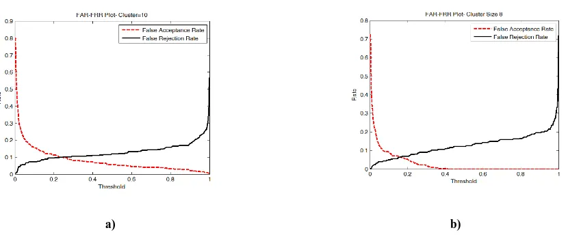
Out of 10 speech samples recorded for each speaker, 5 samples are taken for feature extraction and training. i.e., the input data size for training the network is of size 200 × 65 for a cluster size of 5. ANN is designed and trained for various input cluster sizes of 10, 8, 5 and 4. The False Acceptance Rate (FAR) and False Rejection Rate (FRR) of the system for various clusters are shown in Fig.8 and Fig.9. The Equal Error Rates (EERs) corresponding to each cluster size is shown in Table 5. It is seen that minimum EER is obtained for the cluster of size 5. Hence cluster of size 5 can be considered as the best option for the recognition as the EER is approximately 0.0382 within a matching threshold of 0.152-0.167. Thus the maximum genuine acceptance rate or recognition rate achieved for this system is 96.18%. Also the mean-squared difference (using minimum distance classifier) between the testing and training vectors for various cluster sizes are calculated and the EER obtained with cluster size of 5 is about 0.1662 which is the minimum EER obtained among all the clusters. Thus only 83.38% of recognition rate can be obtained using minimum distance classifier based direct method. The comparison of neural network based and minimum distance based classifiers are shown in Table 6 from which it can be conclude that the neural network method can be adopted for speaker identification with minimum error as the EER is only 3.82% for a cluster size 5.
a) b)
[image:7.595.85.500.538.713.2]a) b)
c)
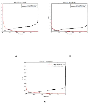
Fig. 7a) FAR-FRR plot for cluster size=7. EER=0.0576 at aThreshold of 0.163-0.166 b) FAR-FRR plot for cluster size=5. EER=0.0382 at a Threshold of 0.152-0.167
[image:8.595.105.446.73.476.2]c) FAR-FRR plot for cluster size=4. EER=0.0452 at a Threshold of 0.1505
Table 5. Cluster Size and EER for ANN method
Cluster Size EER Threshold Range
10 0.0997 0.2320
8 0.0639 0.1625
7 0.0576 0.163-0.166
5 0.0382 0.152-0.167
[image:8.595.336.524.542.668.2]4 0.0452 0.1505
Table 6. Comparison of EER for ANN and Euclidean distance classifier
Cluster Size
EER
Euclidean distance
method
Neural Network method
10 0.2456 0.0997
8 0.2093 0.0639
7 0.1812 0.0576
5 0.1662 0.0382
[image:8.595.77.258.559.631.2]6.
CONCLUSIONS
In this paper speaker recognition technique based on spectral characteristics, mel-frequency cepstral coefficient, was developed. K-means clustering was done to minimize the codebook size. The recognition based on multilayer perceptron classifier and minimum distance Euclidean distance classifier was studied. The Euclidean distance classifier yield only 83.38% of recognition rate while the multilayer perceptron classifier yields 96.18% of recognition rate.
7.
REFERENCES
[1] Thomas F. Quatieri, Discrete Time Signal Processing Principles and Practice, Pearson Education Inc.India. [2] J. P. Campbell, Speaker recognition: A tutorial, Proc.
IEEE, vol. 85, pp. 1437–1462, 1997.
[3] Tomi H. Kinnunen, Optimizing Spectral Feature Based
Text-Independent Speaker Recognition, Academic
Dissertation, University of Joensuu, 2005.
recognition in continuously spoken sentences, IEEE Trans Acoustic, Speech, and Signal Processing, vol 28, no. 4, pp. 357-366,1980.
[5] Hassoun, M. H, Fundamentals of Artificial Neural Networks. MIT Press, Cambridge, MA.
[6] Y.Linde, A.Buzo, and R.M.Gray, An algorithm for
vector quantizer design, IEEE Trans. on
Communications, vol. COM_28 (1), pp.84-96, Jan. 1980. [7] I.A. Basheer, M. Hajmeer, Artificial neural networks: fundamentals, computing, design and application, Journal of microbiological methods 43 (2000) 3–31. [8] Masters, T., 1994. Practical Neural Network Recipes in
C11. Academic Press, Boston, MA.
[9] Haykin S, Neural Networks: A Comprehensive