A Multiple Classifier System for Automatic Speech
Recognition
Sarika Hegde
Department of MCANMAMIT, Nitte
Udupi, Karnataka, India-574110
K.K. Achary
* Professor (Retd.) Dept. of Statistics Mangalore University-574199*
Currently working as Professor of Statistics & Biostatistics, Yenepoya Research Centre, Yenepoya University – 575018.
Surendra Shetty
Department of MCANMAMIT, Nitte
Udupi, Karnataka, India-574110
ABSTRACT
Multiple Classifier System (MCS) is designed by combining two or more classifiers. MCS helps in increasing the accuracy of classification compared to the performance of the individual classifier. In this paper, Multiple Classifier System is implemented for automatic speech recognition. The combined classifier takes the final decision on predicted class label using a class label fuser (also called as classifier fuser). The class label fuser uses the predicted class labels of the two classifiers i.e Hidden Markov Model (HMM) and Support Vector Machines (SVM) and also involves the Dynamic Time Warping (DTW) technique for the final decision on the predicted label. There is an improvement in the accuracy of such classifier compared to the output of any individual classifier.
General Terms
Pattern Recognition, Hybrid System, Intelligent System.
Keywords
Multiple Classifier System (MCS), SVM/HMM, Class label fuser, Kannada Language, Automatic Speech Recognition (ASR)
1.
INTRODUCTION
One can find various classifiers helpful in the area of data mining and pattern recognition where the performance of these classifiers depends on different parameters specific to the classifiers and also the types of applications. It can be said that, there is no single classifier which is best for all types of applications. There is a need, to work out with all types of classifiers and also think of how the specific useful characteristics of individual classifiers can be utilized to solve the problem. Multiple classifier system (MCS) is one such solution working in this direction. MCS also called by different names like, Combining Classifier, Hybrid systems etc., is designed by combining the techniques /results of various classifiers into a single system. Such system can take the advantage of strong aspects of various classifiers and combine these into one system. These are mainly designed for the purpose of improvement in the classifier accuracy. There are different ways in which, classifiers can be combined to design MCS. It can be designed by combining the techniques involved in different classifier into a system called ensemble design. It can also be designed, by developing a module called fuser which combines the output labels of different classifiers [1]. Since, MCS includes more than one classifiers, the implementation is easily suited for parallel programming paradigm.
In this paper, MCS is designed for classifying the sounds in Kannada language. Hidden Markov Model and Support Vector Machine classifiers are used, both of which are trained separately with the same training dataset. While testing, each of these classifier tests the data in parallel. The final decision of classifying the data is implemented in fuser, which also combines the technique of Dynamic Time Warping (DTW). The performance of the MCS classifier is compared with the performance of individual classifiers.
The organization of the rest of the contents of this paper is as follows. The second section briefly highlights the previous works done in the area of MCS/hybrid classifier, especially those related to applications in speech recognition. Section three gives the detail of the feature extraction techniques and also Vector Quantization techniques. In section four, the theoretical aspects of SVM, HMM, DTW classifiers and MCS system are discussed. Description about the dataset and the implementation detail is given in section five. Section six gives a detailed discussion of results based on the implementation of MCS. The last section concludes with a brief summarization and scope for future work.
2.
BACKGROUND
The research in the area of MCS has seen an upward trend in the recent years. It has gained importance mainly due to the advantage of parallel programming which makes efficient use of processing unit in computer and also in increasing classification accuracy.
Early works of combining classifiers were suggested in [2] combining linear and K-nearest neighbor classifier. The approach received greater focus and was described more systematically in [3]. According to [3], combination of multiple classifier algorithms can be of two types; classifier fusion and dynamic classifier selection. Classifier fusion combines the output of individual classifiers run in parallel and dynamic classifier selection predicts the one such classifier which gives the correct output. In the later stages of research many workshops and conferences were organized and categorization of MCS in a more systematic way was considered in [4]. The design of classifier fuser depends on the type of the output generated by the classifier. The outputs can be either the target labels, ranking of each label or the probability vector. Hence, there are many possible variations in the design of fuser.
classifiers output [4], [5]. More categories can be added to the types of combining classifiers like multi-stage organization and sequential approach. Multi-stage organization builds the classifier interactively. There are many stages and iterations where at each stage; the best classifier is selected from the previous stage [6]. MCS also includes sequential approach and parallel approach. In Sequential approach, a classifier is used first and the other ones are used only if the first doesn’t yield a decision with sufficient confidence. For the Parallel approach, all the classifiers are used for the same input example in parallel and the outputs are combined to obtain the final decision. In most of the literature, Hybrid models are created by combining the characteristics of the classifier algorithms like Artificial Neural Network (ANN), SVM, HMM and generating new algorithm called as Hybrid models [7][8][9][10][11].
Since, only two classifiers- SVM and HMM, and a distance calculation technique; DTW are used, most of the above methods cannot be applied directly. All these algorithms generate the output in different ways. SVM generates the output as a list of target labels, HMM generates the output as a list of Maximum Likelihood Probabilities and DTW techniques gives the distance measure as output. Work done in this paper, can be categorized as a combination of parallel and sequential approach [5]. HMM and SVM can be used in parallel in first level and DTW in next level only if the first level doesn’t give satisfactory result.
3.
FEATURE EXTRACTION AND
VECTOR QUANTIZATION
3.1
Mel Frequency Cepstral Coefficients
(MFCC)
In this work, MCS is designed for automatic speech recognition. Sounds of vowels and consonants of Kannada language are recorded and stored in an audio file as dataset. The audio file is divided into number of smaller frames of size of 10ms, which is preprocessed to remove noise. The reconstructed signal after removal of noise is again divided into frames of size 30ms for feature extraction. More details of preprocessing and feature extraction can be found in [12]. The time domain audio data in each frame is denoted as x[n]. Mel Frequency Cepstral Coefficients (MFCC) technique is applied on each frame for computing the feature vector. This feature extraction technique converts the time domain signal into sequence of 12 MFCC coefficients. Following five steps are used in this technique [13][14].
1. Generate DFT coefficients X[k] for the time domain signal x[n]
2. Compute the power spectrum X[m] corresponding to the X[k]
3. Design a series of triangular filters (filter bank) spaced with mel scale
4. Filter the power spectrum with each of the triangular filters
5. Compute the DCT coefficient for the logarithm of the filter-bank energy
The sequence of 12 DCT coefficient values is considered as MFCC feature vector.
3.2
Vector Quantization (VQ) Technique
A vector quantizer maps d-dimensional feature vectors in the vector space Rd into a finite set of vectors V = {v
i: i = 1, 2, ..., K}. Each vector vi is called a code vector or a codeword and the set of all the codeword is called a codebook. Since the audio file is divided into a number of smaller frames, the total
number of frames that is generated depends on the length of the audio file. The number of feature vectors extracted also depends on the length of the audio file. The Vector Quantization technique is used to map the MFCC feature vectors into fixed number of MFCC feature vectors.
Generally, vector of 10 codewords is generated in VQ process. But only five codewords are used since some of the audio sounds of consonants are too short to generate 10 codewords. For each audio file, the vector codebook will be of size 5X12, indicating 5 codewords and 12 MFCC coeffecients.
4.
MULTIPLE CLASSIFIER SYSTEM
(MCS)
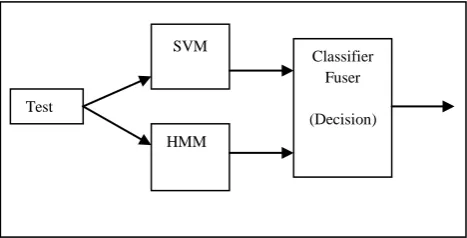
[image:2.595.319.553.356.475.2]MCS is developed with the combination of sequential and parallel approach involving HMM and SVM classifiers and DTW technique. The test data are tested against the individual classifier (SVM and HMM) in parallel. The outputs of each classifier are given to the module called fuser. The fuser logic combines the outputs of each classifier and computes the final predicted target label. In classifier fuser, a technique called DTW is used if found necessary. The working is shown in Figure 1. In this section, working and testing of each classifier and technique used to combine the output in fuser is explained.
Fig 1: HMM/SVM Multiple Classifier System
4.1 Support Vector Machine
Support Vector Machine is a 2-class classifier which is based on statistical learning theory. For the given set of training data, it computes a subset called ‘support vectors’ [15] [16][17]. The set of support vectors identifies the boundary between the observations from different classes. Consider a set of training observations, denoted as (
where corresponds to the values of the attribute set for observation and denotes its class label. The decision boundary can be written in the form:
where, w and b are the parameters of the model. The training phase of the SVM involves estimating the parameters w and b of the decision boundary from the training data. The parameters must be chosen in such a way that the following conditions are met.
Another constraint to maximizing the margin, is equivalent to minimizing the following objective function.
(1)
Test
Data
SVM
HMM
Classifier Fuser
Even though SVM is a two-class classifier, it can be used as multi-class classifier with slight modification. In multi-class classifier, training observation of any one class is considered against training observations of all other classes to compute the support vectors for that class. This is repeated for all the classes one by one. More detail on multi-class SVM classifier can be found in [9].
In the testing process, the test data audio file is preprocessed to divide it into number of frames. For each frame, MFCC feature is computed and then the sequence of features is converted into 5 set vector codebook using Vector Quantization technique. Each feature vector of vector codebook is tested against SVM algorithm for generating the predicted target label. The list of five predicted target labels is generated for each audio file. If only SVM (individual) classifier is used for testing, then the highest occurring target label i.e, modal label is selected as the final predicted target label.
4.2 Hidden Markov Model
A Hidden Markov Model (HMM) is a statistical model in which the system being modeled is assumed to be a Markov chain with unobserved (hidden) states. A Markov chain is a stochastic process in which the future state of the process is based solely on its present state. HMMs are used to specify a joint probability distribution over hidden state sequences
and observed output sequences
. The logarithm of this joint distribution is given by: [15][18].
(2)
The distributions are typically modeled by multivariate Gaussian mixture models (GMMs):
(3)
Where, denotes the Gaussian distribution with mean vector μ and covariance matrix Σ, and M denotes the number of mixture components per GMM. The mixture weights are constrained to be nonnegative and
normalized: for all states j.
Let denote the vector of model parameters including transition probabilities, mixture weights, mean vectors, and covariance matrices. The goal of parameter estimation in the training process in HMMs is to compute the optimal given pairs of observations (feature vectors) and target label sequences , where is the class label. These parameters are computed during training process.
In the testing process, the test audio file is preprocessed in the same way as in SVM, to generate a 5 set vector codebook. This 5-set vector codebook is tested against the HMM model of every class to compute the maximum likelihood probability (MLP). The sequence of MLP values that is computed is same as the number of class labels for each audio file. If only HMM classifier is used for testing, then class label for which MLP is highest is retrieved and selected as the final predicted class label.
4.3
Dynamic Time Warping (DTW)
Technique
This is one of the methods which compute the distance between two sequences of feature vectors of different length and this technique is also used in automatic speech
recognition [19]. The distinguishing feature of this technique is that it creates an alignment between the two sequences and computes the temporal distance. Given that the two speech signals uttering same sounds may differ in length, DTW technique is useful in such situation. The distance is computed between the template frame and the input frame. The training datasets can be considered as the template frames and the test data can be considered as the input frame.
Given two feature vectors sequences and
, the value gives the local distance between the and feature vector. The global distance
is computed recursively using dynamic programming and is given as, [11][20].
(4)
This technique is used in the classifier fuser as the second level of classifier. DTW technique is more useful when there is less number of classes.
4.4 Classifier Fuser Design
As explained in Figure 1, that final decision about the predicted target label is done in the module called Classifier Fuser or Class Label Fuser. Each of the audio data is tested against the SVM and HMM classifier with the technique explained above. Predicted target label computed from individual classifier is compared with each other. If both the classifier’s predicted target labels are matching, then that is considered as the final predicted target label. Otherwise, DTW technique is used to decide the final target label. In case of mismatch, there may be a situation where one of these is correct and another is wrong or both may be wrong. Since this is unknown while testing, we just move forward for further processing. Training data set corresponding to the output target labels of SVM and HMM are retrieved. Then, distance between the training set and the test feature set is computed using DTW technique. Finally, the one with the smallest distance is selected as the final class label.
The following algorithm illustrates the working of fuser logic step by step. The test data is already tested with HMM and SVM individually and output from these is given as input to the fuser.
Algorithm: Classifier Fuser -- To decide final target label Input:
X // test data of size 5X12
T // /training set of size where is the number of class labels and
is the number of audio files in
each class// SVM output predicted target labels for 5-set vector codebook
// HMM output Maximum Likelihood Probabilities
Output:
// final target label
Steps:t1=mode(S) // computes the highest occurring target label in S t2=index(max(H)) // Computes the index of H for which MLP is highest (index corresponds to target label)
if(t1==t2)
// In case of HMM and SVM output labels are same, then final output is decided
y=t1; else
Ct=[t1 t2];
template1=retrieve the training data of class t1 template2= retrieve the training data of class t2 dist1=compute the distance between template1 and test
data dist2=compute the distance between template2 and test
data if dist1<dist2
y=t1 else y=t2 end
The performance of MCS is compared with that of the performance of the individual classifiers and also with the reference combination model called Oracle. The Oracle is defined as an abstract combination model, built such that if atleast one of the individual classifier provides correct answer, then the MCS outputs the correct answer too [1]. Individual classifier performance sets the lower limit for MCS and the performance of the Oracle is an upper bound. The goal of the MCS is to take the classification accuracy to the level of Oracle. It should be noted that Oracle is an imaginary model which can be used for evaluating the classification accuracy of MCS, but not implemented in real time.
5.
DATASET
The recorded sounds of vowels and consonants of Kannada language are considered as the dataset. Each alphabet is considered as a pattern for the classification. The group of 5 vowels and 10 consonants (includes 5 structured and 5 unstructured consonants) of Kannada language are used. The set of structured consonants in Kannada language has five groups and first one from each group is selected. Among unstructured consonants, the first five is selected for the study. The list of vowels and consonants are listed in the following table with their corresponding Unicode name. Forty patterns of each alphabet are recorded with the voice of single female Kannada speaker, creating the database containing around 600 audio clips.
Table 1: Kannada and English representation of list of vowels and consonants used
Consonants
Structured Structured
ಅ (/a/) ಕ್ (/k/) ಯ್ (/y/) ಇ (/i/) ಚ್ (/ch/) ರ್ (/r/) ಉ (/u/) ಟ (/tt/) ಲ್ (/l/) ಎ (/e/) ತ್ (/t/) ಸ್ (/s/) ಒ (/o/) ಪ್ (/p/) ಹ್ (/h/)
6. RESULTS AND DISCUSSIONS
In each of the iteration, hold-out method is used where the dataset is divided randomly in the ratio of 50:50, 25:75 and 75:25. Separate evaluation is done for vowel dataset and consonants dataset. Each audio file in training dataset is converted into MFCC feature vectors and the corresponding Vector codebook is generated. MCS is designed by training the SVM and HMM algorithms using the training dataset. In the process of testing, each audio file of the dataset is first converted into MFCC feature and corresponding vector codebook is generated. This vector codebook is tested using
the designed MCS system, as explained in the previous section.
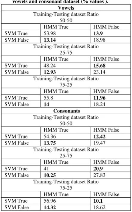
In each experiment, 50 iterations are considered and the performance of SVM and HMM classifiers is observed. As separate classifiers, both SVM and HMM perform almost the same way. The following table shows the classification accuracy of individual classifiers for different vowel and consonant datasets.
[image:4.595.327.549.302.656.2]Each of the table has four entries and the values given are average percentage of correct classification/misclassification over 50 iterations. It can be observed that around 20% of test data in vowel and consonant datasets are misclassified by both HMM and SVM. Around 25% of the test data are misclassified by either HMM or SVM (one of the classifier only). While building MCS advantage of this behavior is taken. The objective is that even if one of the classifier accurately classifies the data, the output should be accurate.
Table 2: HMM/SVM classification true-false table for vowels and consonant dataset (% values ).
Vowels
Training-Testing dataset Ratio 50-50
HMM True HMM False
SVM True 53.98 13.9
SVM False 13.14 18.98 Training-Testing dataset Ratio
25-75
HMM True HMM False
SVM True 48.24 15.68
SVM False 12.93 23.14
Training-Testing dataset Ratio 75-25
HMM True HMM False
SVM True 55.8 11.96
SVM False 14 18.24
Consonants Training-Testing dataset Ratio
50-50
HMM True HMM False
SVM True 54.36 12.42 SVM False 13.75 19.47
Training-Testing dataset Ratio 25-75
HMM True HMM False
SVM True 41 20.9
SVM False 10.25 27.83 Training-Testing dataset Ratio
75-25
HMM True HMM False
SVM True 56.96 10.1
SVM False 14.32 18.62
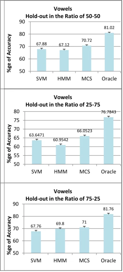
The following graphs in Figure 2 and Figure 3, show the accuracy of classification along with the MCS accuracy. Both the mean and standard error of percentage accuracy over 50 iterations are shown. The following points are observed from the graph,
2. The accuracy of MCS has not reached the accuracy of Oracle.
[image:5.595.327.548.90.516.2]3. The classification accuracy for the dataset of ratio 75:25 is higher compared to 50:50 and followed by 25:75 in all the cases.
Figure 2: The comaprison of classification accuracy of individual classifiers with MCS and Oracle model for
Vowels
There is marginal improvement in classification accuracy using MCS compared to the individual classifiers. Even though the improvement is small, there are two factors to be considered here. First, the data can be tested against individual classifiers using parallel computing resources. The second point is that, DTW is used only in second level if there is a disagreement in the outputs of the HMM and SVM. In DTW also, distance of the test data is computed with only two template training data. If parallel computing resources are utilized, then improvement in classification accuracy can be
[image:5.595.67.281.144.616.2]achieved with computational economy.
Figure 3: The comaprison of classification accuracy of individual classifiers with MCS and Oracle model for
Consonants
7. CONCLUSIONS
A Multiple Classifier System is designed and implemented which uses combined approach of parallel and sequential classifier. HMM and SVM classifier are in parallel individually which is cascaded with DTW, a distance computing technique. The decision logic for cascading the outputs of HMM and SVM is designed in the module named class label fuser or classifier fuser. The system is applied on the vowel and consonant datasets of Kannada language. The implementation of the system is simple and it achieves an improvement in the classification accuracy. Further improvements in the system in terms of fuser logic improvements and feature selection and mixing strategies are in progress.
8. REFERENCES
[1] Wozniak, M., Grana, M., Corchado, E., (2014). A survey of multiple classifier systems as hybrid systems. Information Fusion, Vol 16(2014), pp 3-17.
67.88 67.12 70.72
81.02
50 60 70 80 90
SVM HMM MCS Oracle
%
ge
o
f A
cc
u
rac
y
Vowels
Hold-out in the Ratio of 50-50
63.6471
60.9542
66.0523
76.7843
50 55 60 65 70 75 80
SVM HMM MCS Oracle
%
ge
o
f A
cc
u
rac
y
Vowels
Hold-out in the Ratio of 25-75
67.76 69.8 71
81.76
50 60 70 80 90
SVM HMM MCS Oracle
%
ge
o
f A
cc
u
rac
y
Vowels
Hold-out in the Ratio of 75-25
66.78 68.11
73.05
80.53
50 60 70 80 90
SVM HMM MCS Oracle
%
ge
o
f A
cc
u
rac
y
Consonants
Hold-out in the Ratio of 50-50
61.9085
51.2614
65.2614
72.1634
50 55 60 65 70 75
SVM HMM MCS Oracle
%
ge
o
f A
cc
u
rac
y
Consonants
Hold-out in the Ratio of 25-75
67.06 71.28
74.12
81.38
50 60 70 80 90
SVM HMM MCS Oracle
%
ge
o
f A
cc
u
rac
y
Consonants
[2] Dasarathy, B, V., and Sheela, B, V., (1978). A Composite Classifier System Design: Concepts and Methodology. Proceedings of IEEE, Vol 67:708-713, 1978.
[3] Woods, K., Kegelmeyer, W, P., and Bowyer, K., (1997). Combination of multiple classifiers using local accuracy estimates. IEEE Transactions on Pattern Analysis & Machine Intelligence. Vol 19:405-410, 1997.
[4] Kuncheva, L, I., (2004). Combining Methods and Algorithms. John Wiley & Sons, New Jersey, 2004
[5] Saez, J, A., Galar, M., Huengo, J., and Herrera, F., (2013). Tackling the Problem of Classification with Noisy Data using Multiple Classifier System: Analysis of the Performance and Robustness. Int. J. of Information Sciences, Vol 247 (1-20), 2013.
[6] Ho, T, K.., Hull, J, J., and Srihari, S, N., (1994). Decision Combination in Multiple Classifier Systems. IEEE Transaction on Pattern Analysis & Machine Intelligence, Vol 16, pages 66-75, 1994.
[7] Ganapathiraju, A., and Picone, J., (2000). Hybrid SVM/HMM Architectures for Speech Recognition, ICSLP2000, 2000
[8] Axelrod, S. and Maison, B. (2004). Combination of Hidden Markov Models with Dynamic Time Warping for Speech Recognition. In Proceedings of IEEE ICASSP, pages 173–176, 2004.
[9] He, X., and Zhou, X., (2005). Audio Classification by Hybrid Support Vector Machine / Hidden Markov Model. UK World Journal of Modeling and Simulation, ISSN 1746-7233, England, Vol. 1, No. 1, 2005, pp. 56-59.
[10] Kruger, S, E., Schaffoner, M., Katz, M., Andelic, E., and Wendemuth, A. (2005). Speech Recognition with Support Vector Machine in a Hybrid System, In Interspeech, pages 993-996.
[11]Bourouba, E-H., Bedda, M., and Djemili, R., (2006). Isolated Word Recognition System based on Hybrid
Approach DTW/GHMM. Informatica, Vol 30, pages 373-384, 2006
[12] Hegde, S., Achary, K. K., Shetty, S., (2012). Isolated Word Recognition for Kannada Language Using Support Vector Machine. Int Conference on Information Processing 2012, CCIS 292 , Vol 292, 262–269.
[13] Rabiner, L., and Juang, B-H (1993). Fundamentals of Speech Recognition, Prentice Hall PTR, ISBN:0-13-015157-2. NY, USA, 1993.
[14]Slaney, M., (1998). Auditory toolbox: A MATLAB Toolbox for auditory modeling work, Tech. Rep. 1998-010, Interval Research Corporation, Palo Alto, Calif, USA, 1998, Version 2.
[15] Alpaydin, E., (2004). Introduction to Machine Learning, PHI Publications, ISBN-81-203-2791-8.
[16] Duda, R. O, Hart, P. E., and Stork, D. G., (2006). Pattern Classification, Wiley Publication
[17]Tan, P., Steinbach, M., and Kumar, V., (2006). Introduction to Data Mining, Pearson Addison Wesley, ISBN: 978-81-317-1472-0.
[18]Sha, F., & Saul, L. K. (2009). Large Margin Training of Continuous Density Hidden Markov Models. In J. Keshet and S. Bengio (Eds.), Automatic speech and speaker recognition: Large margin and kernel methods. Wiley-Blackwell.
[19]Godin, C., and Lockwood, P., (1989). DTW schemes for continuous speech recognition: a unified view. Comp. Speech and Lang., vol. 3, no. 2, pp. 169–198, 1989
[20]Wachter, M, D., Demuynck, K., Compernolle, D. V., and Wambacq, P., (2003). Data driven example based continuous speech recognition,” in Proceedings of Eurospeech, pages 1133-1136, Geneva, Switzerland, September 2003.