Normalized Scale Coding for Geometrical Coding in
Image Retrieval System
S. Vyshali
Research scholar Assistant professor
GPREC,Kurnool.
M.V.Subramanyam, Ph.D
Supervisior Principal
SREC,Nandyal.
K.Soundara Raajan, Ph.D
Co-Supervisior Retd. Professor JNTU,Anantapur.
ABSTRACT
Pattern recognition has emerged as an effective measure for automated system. I n such an approach the coding is carried out over a set of images and result are retrieved based on the best match approach. Where image features are taken as the representative feature for image coding, the introduced artifacts are the major effects at the coding level. In this work a shape oriented coding based on curvature coding and its representation based on Normalized information is proposed. The coding reveals the lower spectral information of the image contour and considers it as feature information which improves the recognition approach.
Keywords
Pattern recognition, image coding, normalized coding, curvature coding.
1. INTRODUCTION
Information is basically represented in multimodal features. Humans can efficiently and effectively process information simultaneously in multiple dimensions. These multiple media that aid effective communication can be characterized into speech, audio, image, video, and textual data. Advances in computing and networking are generating a significant amount of interest in multimedia services and applications. Powerful processors, high-speed networking, high-capacity storage devices, improvements in compression algorithms, and advances in processing of audio, speech, image, and video signals are making image systems technically and economically feasible in image recognition. Various applications in image recognition and image databases have been described in the literature. Much of the past research in image retrieval has concentrated on the feature extraction stage. For each database image, a feature vector which describes various visual cues [1], such as shape, texture, or color [1,3] is computed. Given a query image, its feature vector is calculated and those images, which are most similar to this query based on an appropriate distance measure in the feature space, are retrieved. The traditional image matching methods based on image distance or correlations of pixel values are in general too expensive and not meaningful for such an application. The methods proposed in past for image recognition can be broadly classified into two categories on the basis of the approach used for extracting the image attributes. The spatial information preserving methods [4,8] derive features that preserve the spatial information in the image. It is possible to reconstruct the image on the basis of
these feature sets. Representative techniques include polygonal approximation of the object of interest [5, 6], physics-based modeling and principal component analysis (PCA). The non-spatial information [7] preserving methods extract statistical features that are
used to discriminate among objects of interest. These include heuristics based on edge angle histograms, and other ad hoc shape measures [10, 12]. These techniques were suggested for greater accuracy at a cost of heavy computation or faster operation with lesser accuracy. In the following sections, we briefly review the existing invariant moment based recognition method. In this paper, we address the problem of an efficient and accurate retrieval from a large image database based on image content of its shape. Since we desire a system that has both high speed and high accuracy of retrievals a curvature based recognition algorithm for image recognition is proposed. The curvature coding is carried out over a evolved contour. The contour coding is processed with normalize coding to generate a finer feature description.
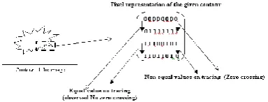
2. CONTOUR CODING
Contours are defined as the bounding regions of an image. Contour defines the shape, region and edge region in images. The process of edge estimation by edge operators were analyzed in previous section. It is observed that during compression as image is processed in blocks, blocking artifacts are generated. These artifacts are been minimized by tracing the edge regions, so as the edge artifacts are nullified. In previous section it is seen that working over edge with filtration reduces the visual artifacts. However the system overhead due to edge estimation and filtration process has not been considered. The edge estimated and processed in such system are lost at the bounding region in a block due to lossy compression and because of block processing. Where as in a contour is estimated in a continuous tracing over the image, hence such coding is more informative for region description than the edge descriptor.
(a)
(b)
(c)
Fig 1 (a) Original image sample, (b) Extracted Edge region using canny operator, (c) Extracted contour region.
(a) (b)
(c)
Fig 2 (a) enlarged section of the original sample, (b) Estimated edge of the region, (c) Estimated contour region
Figure illustrates the extracted bounding region for the given image sample. Figure1 (b) shows the extracted edge region using canny operator and Figure2(c) shows the extracted contour for the same image. Figure2 illustrates the enlarge version of figure1. It is observed from Figure2 (b) that the bounding region obtained by the edge estimation operator result in disjoints due to loss of information. While the bounding region derived by contour estimation results in a continuous bounding region. This estimation results in higher edge preserving, results in minimization of visual artifacts.
2.1 Contour Evolution
Contour is defined as outermost continuous bounding region of a given image. For the detection of contour evaluation all the true corners should be detected and no false corners should be detected. All the corner points should be located for proper continuity. The contour evaluator must be effective in Estimating the true edges under different noise levels for robust contour estimation. For the estimation of the contour region an 8-region neighborhood-growing algorithm is used as illustrated below.
2.2
8-Region
Neighborhood
growing
algorithm
1.Find outermost initial pixel of an edge by vertical or horizontal scanning for obtained edge information. 2.The obtained initial pixel is taken as reference and is
termed as seed pixel.
3. Taking seed pixel as starting co-ordinate, find eight adjacent neighbors of it tracing in anti-clock wise direction.
4.The possible tracing order is as shown in figure 5.3. 5.If the obtained seed coordinate is taken as (x,y) then the
scanning order is, [1. (x+1, y), 2. (x+1, y+1), 3. (x,y+1), 4. (x-1, y+1), 5. (x-1, y), 6. (x-1, y-1), 7. (x,y-1), 8. (x+1, y-1)].
[image:2.595.95.205.70.201.2]6.In case of the current pixel is found to be the next adjacent neighbor, update-the current pixel as new seed pixel and repeat step 3,4 and 5 Recursively until the Initial seed pixel is reached.
Fig 3: probable scanning order for 8-Region neighborhood-growing algorithm
The tracing order is coded for path tracing in frame formation, wherein the tracing orientation is given values defined by,
Fig 4: Issued Orientational weight value for contour tracing
While contour evolution for every forward / backward tracing a value is assigned, this is buffered as a stream of information. This sequence of data formulates the frame for encoding then sequence for storage.
3. CONTOUR SCALE SPACE CODING
Shape representation methods for planar curves previously proposed in computational vision fail to satisfy one or more of the criteria outlined above. Note, however, that each may be quite suitable for special-purpose shape representation and recognition tasks. The Hough transform has used to detect lines, circles, and arbitrary shapes. Edge elements in the image vote for the parameters of the objects of which they are parts. The votes are accumulated in a parameter space. The peaks of the parameter space then indicate the parameters of
segmented region of the Image
Reference Seed Pixel
( x , y )
.
1 2
4 5 6 7
.
.
.
.
.
1 2 Contour trace
Corners
.
. . .
3 4
5
6
[image:2.595.53.209.244.475.2] [image:2.595.318.526.283.416.2] [image:2.595.373.483.480.565.2]the objects searched for, Chain encoding, techniques approximate a curve using line segments lining on a grid. Polygonal approximations of a curve are computed by using various criteria to determine “breakpoints” that yield the “best” polygon. The medial axis transform, computes the Skelton of a 2-D object by a thinning algorithm that preserves region connectivity. Shape factors and quantitative measurements of the object such as area, perimeter, and compactness as a description of its shape. Strip trees, are a set of approximating polygons ordered such that each polygon approximates the curve with less approximation error than the previous polygon. Splines represent a curve using a set of analytic and smooth curves. The smoothing splines method parameterized the curve to obtain two coordinatefunctions. Cross-validate regulation is then used to arrive at an “optimal” smoothing of each coordinate function. A new shape representation is computed by convolving a path-based parametric representation of the curve with a Gaussian function, as the standard deviation of the Gaussian varies from a small to a large value and extracting the curve plane noise occurs in the resulting curves. The representation is essentially invariant under rotation, uniform scaling, and translation of the curve. This and a number of other properties makes it suitable for recognizing a noisy curve of arbitrary shape at any orientation, The process of describing a curve at increasing levels of abstraction is referred to as the evolution of that curve.
3.1 Curve plane evolution
To evaluate the curve plane for the obtained contour of given image following approach is made, For a given a contour co-ordinates (x (u), y(u)) the curve plane of the given contour is given by,
(1)
Where are first derivative of given contour co-ordinates and are the double derivative of x and y. For the obtained curve plane, 1-D contour is obtained by applying smoothening operation to reduce the noise in bounding contours. The smoothening is continued by incrementing the Gaussian values (σ) on the obtained contour until no noise exist.
4. PROPOSED SCALED CODING
REPRESENTATION
A planar curve is a set of points whose position vectors are the values of a continuous, vector-valuedfunction. It can be represented by the parametric vector equation,
(2)
The function r(u) is a parametric representation of the curve. Planar curve has an infinite number of distinct parametric representations. A parametric representation in which the parameter is the arc length‘s’ is called a natural parameterization of the curve. A natural parameterization can be computed from an arbitrary parameterization using the following equation:
(3)
Where ŕ represents the derivative. i.e., ŕ = dr/dv. For any parameterization
(4)
(5)
Differentiating the expression for t (u), we obtain
(6)
It now follows that
(7)
Therefore, it is possible to compute the curve plane of a planar curve from its parametric representation. Special cases of the parameterization yield simplifications of these formulas. If w is the normalized arc length parameter, then
(8)
Given a planar curve
(9)
Where w is the normalized arc length parameter, an evolved version of that curve is defined by
(10)
Where
Denotes a Gaussian of width σdefined by
(11)
and are explicitly defined by
(12)
(13)
The curve plane of is given by
(14)
Where
(15)
(16)
(17)
(18)
The process of generating the ordered sequence of curves {Γσ│σ>=0} is referred to as the evolution of Γ.
increasing values of σ. Note that when a planar curve evolves according to the process defined above, its total arc length shrinks. The amount of shrinkage is directly proportional to the value of σ.
(a)
[image:4.595.335.521.72.143.2](b) (c)
Fig 5: Outliner region of generic leaf sample
(d) (e)
[image:4.595.94.242.126.452.2](f)
Fig 6: The region smoothening during evolution of a sample pattern used at: (a) σ =2 ,(b) σ = 4 , (c) σ =8, (d) σ =
16, (e) σ = 32, (f) σ = 64.
In certain applications, this may be an undesirable feature. For example, the evolution process defined above may be used to smooth edges extracted from an image by an edge detector. However, it may be advantageous to have the smoothed edges as close as possible to the physical location of the original edges. This can be accomplished by estimating the amount of movement at each point on the smoothed edges and adding a vector tothe location vector of that point to compensate for that movement. The result is a smoothed curve that is physically closer to the original curve.
(19)
Where, X= conv(x,g) and Y=conv(y,g)
g is Gaussian distribution function and u is the arc length parameter. X' and Y' are the first order derivative of X,Y and X'',Y'' are the second order derivatives.
The curve plane smoothening operation is as shown Fig.7.
Fig 7: Curve plane smoothening operation at variable
For the obtained smoothened curve plane at each Gaussian level, noise are computed.
4.1 Crossover Evaluation
After smoothening the given curve plane noise is evaluated, where the noise is found when the tracing come across a pixel variation from 0 to 1 or 1 to 0 level. The operation is as illustrated in Fig.8.
Fig 8: Noise computation operation for an obtained curve plane
Once the noise cross were obtained they are buffered for a corresponding arc length (u) and given Gaussian value (σ), once all the noise were found they are been plotted for arc length v/s sigma value as shown in Fig.9
Fig 9: NCC plot for a given curve plane
From the obtained NCC plot important curve plane features are extracted. To obtain the important curve plane feature a threshold is set given by Threshold (T) = 0.6 * max. Peak value. This indicates that a NCC peak of more than 60% of the obtained curve plane information is used for image feature representation. This approach eliminates the consideration of lowerpeaks resulting in elimination of shape information generated due to external noises. This noise used to be reduced by filtration approach in conventional methods. The proposed image coding approach integrally minimizes the edge distortions representation with effective image contour representation for image samples.
The proposed algorithm for normalize contour coding is summarized as,
Step 1: read an image
[image:4.595.333.525.276.349.2] [image:4.595.339.516.446.542.2]Step 3: apply 8-neighbourhood region method to extract contour
Step 4: open the contour from seed as 1-D array
Step 5: evaluate the curvature in this array, curvature is defined by k.
Step 6: proceed curvature evaluation with smoothening of evaluation Curvature with variation in Gaussian factor (σ) Step 7: repeat until all curvature are smoothened.
Step 8: plot a relational graph of pixel position over smoothening Gaussian for existing curvature
Step 9: compute a threshold Th= max(peak) * k
Where K is the limiting tolerance factor
Step 10: for the obtained Th value a decision condition is
applied as, ifPi,j<Th , Pi,j = 0;
else Pi,j= Pi,j
wherePi,j is the obtainedcurvature element.
The pseudo code for the proposed coding algorithm is as presented below,
Algorithm NCC( ) {
read image ; convert( x, y ); eight_neighbour( ); contour[m,n ]; //for
//evaluate the curvature by using k for i= 1 to n
k[u,i] ={ X[u,i] * Y[u,i] – X[u,i]*Y[u,i]}/(X[u,i]**2 + Y[u,i]**2)**.05
plot pixel( );
//compute threshold value Th = (max(peak) *k)/100 if ( P[I,j]<Th) then P[I,j]=0;
else
P[I,j]=P[I,j]; }
5. RESULT OBSERVATIONS
This section provides the complete illustration about the evaluation of performance of proposed approach. It also gives the comparative analysis by comparing the proposed approach with the previous approaches.
Fig 10. Illustrates the processing sample used as query. The derived contour for the query sample is illustrated in fig.10(a). The comparative results obtained after decoding using conventional contour coding and spectral contour coding along with filtration is presented in fig.10(b) and fig10(c). The obtained observations clearly illustrate that by the usage of NCC algorithm edge artifacts is considerably minimized in comparison to contour coding.
(a) (b) (c)
Fig 10: a) Noise image b) image from contour coding c) Noise free image using filtration and NCC algorithm
The above figure gives the visual analysis, i.e. by just observing it is able to analyze that the proposed method is better. The following figures the numerical evaluation by evaluating the recall rate, estimation accuracy and also computation time. These also give the comparative analysis for the proposed approach with the previous approaches.
Fig 11 : Recall rate versus bpp
The above figure illustrates the performance of the proposed approach with the evaluation of recall rate versus bpp. From the figure it is clear that with increasing the bpp the recall rate is going to be decreased. It also illustrates that the recall rate for the proposed method is better compared to JPEG and contour coding.
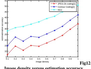
Fig12: Image density versus estimation accuracy
The above figure illustrates the performance of the proposed approach with the evaluation of estimation
accuracy versus image density. From the figure it is clear that with increasingthe image density the estimation accuracy is going to be increased. It also illustrates that the estimation accuracy for the proposed method is better compared to JPEG and contour coding.
0.1 0.2 0.3 0.4 0.5 0.6 0.7 0.8 0.9 1 30
35 40 45 50 55 60 65 70 75
bpp-coding
R
e
c
a
ll
r
a
te
JPEG-2k-coding[1] Contour Coding[2] NCC
0.1 0.2 0.3 0.4 0.5 0.6 0.7 0.8 0.9 1 5
10 15 20 25 30 35 40 45 50 55
image density
e
s
ti
m
a
ti
m
a
ti
o
n
a
c
c
u
ra
c
y
[image:5.595.362.520.163.301.2] [image:5.595.349.533.406.545.2]Fig 13: Comparision plot for computation times taken
The above figure gives the comparative analysis of the proposed approach with the JPEG and contour coding approaches under the regard of total time taken for the evaluation. From the computation time taken by the proposed approach is very low compared to previous approaches thus the NCC method is efficient. The conclusions are provided in next section.
6. CONCLUSION
This paper outlines the proposed method using NCC algorithm. By the scaled approach of extracted contour in 1-D a minimization in noise level at the bounding regions are observed. The approach of NCC minimizes the filtration effort with the usage of a minimum thresholding for obtained scaled plot. This approach eliminates the edge artifacts on the assumption of a threshold limit. With the approach of developed method the recall rate of the system is observed to be improved in comparison to the existing recognition approach of shape based CSS approach. The NCC approach normalizes the enveloped contour hence redefines the bounding region for the test sample. With the approach of NCC an improvement in the recognition efficiency is observed.
7. REFERENCES
[1] H. Asada and M. Brady, “The curvature primal sketch,” IEEE Trans, Pat, Anal.Machine Intell, vol, PAMI-8 pp. 2-14, 1986.
[2] D.H. Ballard, “Generating the Hough Transform to detect arbitary shapes” PattRecogn., vol. 13 pp. 111-122, 1981.
[3] D.H. Ballard and C.M. Brown, Computer Vision. Engle Cliffs, NI: Prentice –Hall, 1982.
[4] H. Bluem, “Biological shape and visual science (part I),” J. Theoretical Biol., vol. 38, pp. 205-287, 1973.
[5] P. E. Danielsson, “A new shape factor,” CGIP, vol. 7, pp. 292-299, 1978.
[6] L. S. Davis, “Understanding shape: Angles and sides,” IEEE Trans. Comput., vol. C-26, pp. 236-242, 1977.
[7] R. O. Duda and P.E. Hart, “Use of the Hough transformation to detect lines and curves in pictures,” Comm.ACM, vol.15, pp. 11-15, 1972.
[8] H. Freeman, “Computer processing of line-drawing images,” Comput Surveys, vol, 6, 1974.
[9] M. Gage and R.S. Hamilton, “The heat equation shrinking convex phanc curves,” J. Differential Geometry, vol. 23, pp.69-96, 1986.
[10] A. Goetz, Introduction to Differential Geometry. Reading, MA: Addison-Wesley, 1970.
[11] R. M. Haralick, A. K. Mackworth, and S. L. Tanimoto, “Computer Vision update,” Tech.Rep, 89-12, Dept. Comput. Sci. Univ. British Columbia, Vancouver , 1989.
[12] J. Hong and X. Tan, “Recognize the similarity between shapes under affine transformation,” in Proc. ICCV(Tampa, FL), 1988, pp. 489-493.
[13] B. K. P. Horn and E. J. Weldon, “Filtering closed curves,” IEEE Trans Patt. Anal.Machine Intell, vol. PAMI-8, pp. 665-668, 1986.
[14] P. V. C. Hough, “Method and means for recognizing complex patterns,” U.S. patent 3 069 654, 1962. [15] R. A. Hummel, B. Kissia, and S. W. Zucker, “Debluring
Gaussian blur,”CVGIP, vol. 38, pp. 66-80, 1987.
[16] W. Kecs, The Convolution Product and Some Applications. Boston, MA: D. Reidel, 1982.
[17] B. Kimia, A. Tannenbaum, and S.W. Zucker, “Toward a computational theory of shape: An overview,” TR-CIM-89013, McGill Univ., 1989
1 2
0 5 10 15 20 25 30 35 40 45 50
Methods
C
o
m
p
u
ta
ti
o
n
T
im
e
(S
e
c
)