Simulating the influence of snow surface processes on soil moisture dynamics and streamflow generation in an alpine catchment

(1)

https://doi.org/10.5194/hess-21-4053-2017 © Author(s) 2017. This work is distributed under the Creative Commons Attribution 3.0 License.

Simulating the influence of snow surface processes on soil moisture

dynamics and streamflow generation in an alpine catchment

Nander Wever1,2, Francesco Comola1, Mathias Bavay2, and Michael Lehning2,1

1_{École Polytechnique Fédérale de Lausanne (EPFL), School of Architecture, Civil and Environmental Engineering,} Lausanne, Switzerland

2_{WSL Institute for Snow and Avalanche Research SLF, Davos, Switzerland}

Correspondence to:Nander Wever ([email protected])

Received: 16 November 2016 – Discussion started: 17 January 2017

Revised: 29 June 2017 – Accepted: 14 July 2017 – Published: 14 August 2017

Abstract. The assessment of flood risks in alpine,

snow-covered catchments requires an understanding of the linkage between the snow cover, soil and discharge in the stream net-work. Here, we apply the comprehensive, distributed model Alpine3D to investigate the role of soil moisture in the pre-disposition of the Dischma catchment in Switzerland to high flows from rainfall and snowmelt. The recently updated soil module of the physics-based multilayer snow cover model SNOWPACK, which solves the surface energy and mass balance in Alpine3D, is verified against soil moisture mea-surements at seven sites and various depths inside and in close proximity to the Dischma catchment. Measurements and simulations in such terrain are difficult and consequently, soil moisture was simulated with varying degrees of suc-cess. Differences between simulated and measured soil mois-ture mainly arise from an overestimation of soil freezing and an absence of a groundwater description in the Alpine3D model. Both were found to have an influence in the soil mois-ture measurements. Using the Alpine3D simulation as the surface scheme for a spatially explicit hydrologic response model using a travel time distribution approach for inter-flow and baseinter-flow, streaminter-flow simulations were performed for the discharge from the catchment. The streamflow sim-ulations provided a closer agreement with observed stream-flow when driving the hydrologic response model with soil water fluxes at 30 cm depth in the Alpine3D model. Perfor-mance decreased when using the 2 cm soil water flux, thereby mostly ignoring soil processes. This illustrates that the role of soil moisture is important to take into account when under-standing the relationship between both snowpack runoff and

rainfall and catchment discharge in high alpine terrain. How-ever, using the soil water flux at 60 cm depth to drive the hy-drologic response model also decreased its performance, in-dicating that an optimal soil depth to include in surface sim-ulations exists and that the runoff dynamics are controlled by only a shallow soil layer. Runoff coefficients (i.e. ratio of rainfall over discharge) based on measurements for high rainfall and snowmelt events were found to be dependent on the simulated initial soil moisture state at the onset of an event, further illustrating the important role of soil moisture for the hydrological processes in the catchment. The runoff coefficients using simulated discharge were found to repro-duce this dependency, which shows that the Alpine3D model framework can be successfully applied to assess the predis-position of the catchment to flood risks from both snowmelt and rainfall events.

1 Introduction

(2)

2003; Berg and Mulroy, 2006; Seyfried et al., 2009; Koster et al., 2010). Additionally, rain-on-snow events may signifi-cantly increase the liquid water outflow from the snowpack (Mazurkiewicz et al., 2008; Wever et al., 2014a; Würzer et al., 2016, 2017) and many flooding events have been caused by such events (Marks et al., 2001; Rössler et al., 2014).

However, accurate simulations of liquid water draining from the snowpack due to snowmelt or rainfall (henceforth termed snowpack runoff) are not sufficient to understand catchment runoff. The degree of saturation of the soil was found to determine the eventual effect of snowpack runoff on streamflow (McNamara et al., 2005; Seyfried et al., 2009; Bales et al., 2011). This effect is not limited to snowpack runoff, but is also found for rainfall (Bales et al., 2011; Penna et al., 2011). During the winter months, the snow cover ba-sically decouples the soil from the atmosphere and the upper boundary for the soil is determined by the state of the snow cover on top (McNamara et al., 2005; Kumar et al., 2013). Often, the hydrological processes are strongly reduced dur-ing wintertime, such as groundwater flow and streamflow, until the spring snowmelt provides liquid water again to the hydrological system. A model system to assess the hydro-logic response of a catchment is therefore required to simu-late both the soil and the snowpack accurately.

To assess this coupling between snowmelt, soil moisture and streamflow, the use of physics-based models of snow sur-face process descriptions in hydrological models seems at-tractive as they should not require calibration for the specific application. For example, Rigon et al. (2006) show that the physics-based hydrological model GEOtop, which includes a relatively simple physics-based snow scheme, is able to pro-vide accurate streamflow simulations for small catchments, where a snow cover is present for extended periods during the winter season. Kumar et al. (2013) also found that using a physics-based model approach for snow related processes in the Penn State Integrated Hydrologic Model (PIHM) model achieved a slightly better performance for streamflow sim-ulations than a temperature index approach. The results in their study suggest that this improvement is linked to the spatial variability of snow distribution and snowmelt, which provides a strong control on other components of the hydro-logical cycle, like soil moisture or streamflow. In Warscher et al. (2013), a similar comparison was made by comparing a temperature-index approach with an energy balance ap-proach to determine snowmelt in the physics-based hydro-logical model WaSiM-ETH. Their results show that the en-ergy balance approach provides improvements particularly at the small spatial scales typical of high alpine headwa-ter catchments. However, the improvements rapidly decrease with increasing scale. It has been argued that simple temper-ature index based snowmelt models may perform well af-ter careful calibration (Kumar et al., 2013; Comola et al., 2015a) and those models are still commonly used in oper-ational flood forecasting. Nevertheless, physics-based snow

models may be considered more reliable when extrapolating to other conditions such as for climate change scenarios (e.g. Bavay et al., 2013) or to catchments where limited calibra-tion data are available.

The fully distributed Alpine3D model is typically applied for detailed studies of small scale surface processes in alpine catchments where snow plays an important role (Lehning et al., 2006; Mott et al., 2008; Groot Zwaaftink et al., 2013). In alpine terrain, considering the length scales less than a few 100 m is important as on these scales, wind drifts determine the snow accumulation and local topography heavily influ-ences the energy balance via the slope aspect, angle and local shading. In this study, the recent addition to the SNOWPACK model of a solver for Richards Equation for soil (see Wever et al., 2014a, 2015) is verified against soil moisture measure-ments in the vicinity of Davos, Switzerland. The SNOW-PACK model provides the surface scheme in the Alpine3D model framework, using physics-based descriptions of soil-snow-vegetation processes (Gouttevin et al., 2015). Here, the capabilities of Alpine3D to capture the soil moisture state is assessed. Furthermore, the Alpine3D model provides the surface scheme for a travel time distribution hydrologic response model to simulate catchment discharge (Comola et al., 2015b; Gallice et al., 2016) and here the role of soil moisture in the coupling of Alpine3D to the hydrologic re-sponse model, as well as the influence of the soil moisture state on streamflow generation in the catchment is investi-gated.

2 Study area and data

2.1 Study area

(3)

[image:3.612.127.470.64.405.2]

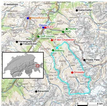
Figure 1.Topographical map of the simulated domain, showing the locations of the stations. Interkantonales Mess- und Informationssys-tem (IMIS) stations are shown in black, Interregionales KriseninformationssysInformationssys-tem (IRKIS) stations in red, SensorScope stations in green, SwissMetNet stations in blue and Weissfluhjoch in brown. The Dischma catchment and the gauging station measuring streamflow in the Dischmabach at the outlet of the Dischma catchment are shown in cyan. The inset shows the location of the simulation domain (red square) in Switzerland. Maps were reproduced by permission of swisstopo (JA100118).

from 1 October 2004 to 30 September 2014, with a special focus on the period from 1 October 2010 to 30 September 2013, during which soil moisture measurements were col-lected.

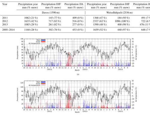
Snowfall plays an important role in the Davos area. Table 1 shows the precipitation sums for two heated rain gauges at two elevations in the region. About 40 to 80 % of total precip-itation falls as snow at the lower and upper parts of the Dis-chma catchment, respectively (Zappa et al., 2003). Precipita-tion in the Davos area is commonly separated into rain and snowfall based on an air temperature threshold of 1.2◦C. The winter months are dominated by snowfall at all elevations in the area. In the meteorological summer months (June– August), about 7 % of the precipitation amounts still consist of snowfall at 2536 m a.s.l. At the lower rain gauge, almost all precipitation falls as rain in the meteorological summer months. The two precipitation gauges show a strong eleva-tion gradient in precipitaeleva-tion: at 2536 m a.s.l., precipitaeleva-tion amounts are about 1.4 times higher than at 1590 m a.s.l. This

elevation gradient may, however, overestimate the true areal-mean gradient because the upper site may be limited in repre-sentativeness for the Dischma catchment (Wirz et al., 2011; Grünewald and Lehning, 2015). Furthermore, the area ex-hibits a climatological northwest–southeast gradient in pre-cipitation (Vögeli et al., 2016).

Figures 2a and b show the daily temperature and precip-itation amounts separated in snowfall and rainfall for both locations with a heated rain gauge. The yearly cycle in tem-perature has a similar amplitude at both elevations. Max-imum daily temperatures occasionally surpassed 20◦C at 1590 m a.s.l. and 15◦C at 2536 m a.s.l. The minimum daily temperatures reached −20 and −25◦C, respectively. Note that those low temperatures were reached after significant snowfall in the months before. Therefore, the isolating snow cover is expected to have prevented an impact of these cold days on soil freezing.

(4)

dom-Table 1.Yearly, winter months (DJF) and summer months (JJA) precipitation sums from heated rain gauges in the area around Davos. In

brackets is the percentage that falls as snow, based on measured air temperature below 1.2◦C calculated with half-hourly measurements. The

last line lists the average over the 10-year period (2005–2014).

Year Precipitation year Precipitation DJF Precipitation JJA Precipitation year Precipitation DJF Precipitation JJA

mm (% snow) mm (% snow) mm (% snow) mm (% snow) mm (% snow) mm (% snow)

Davos (1590 m) Weissfluhjoch (2536 m)

2011 1062 (21 %) 145 (77 %) 409 (0 %) 1368 (47 %) 184 (95 %) 491 (7 %)

2012 1633 (42 %) 717 (83 %) 516 (0 %) 2337 (63 %) 1096 (100 %) 722 (6 %)

2013 1085 (28 %) 261 (82 %) 277 (0 %) 1590 (48 %) 400 (98 %) 476 (11 %)

2005–2014 1168 (28 %) 302 (76 %) 453 (0 %) 1659 (52 %) 440 (97 %) 648 (7 %)

0 10 20 30 40 50 60 70 80 90 100

10 11 12 1 2 3 4 5 6

(2011)7 8 9 10 11 12 1 2 3 4 (2012)5 6 7 8 9 10 11 12 1 2 3 4 (2013)5 6 7 8 9

−25 −20 −15 −10 −5 0 5 10 15 20 25

Precipitation (mm) _{Air temperature (}

°

C)

Month Rain

Snow Air temperature

0 20 40 60 80 100 120

10 11 12 1 2 3 4 5 6

(2011)7 8 9 10 11 12 1 2 3 4 (2012)5 6 7 8 9 10 11 12 1 2 3 4 (2013)5 6 7 8 9

−25 −20 −15 −10 −5 0 5 10 15 20

Precipitation (mm) _{Air temperature (}

°

C)

Month Rain

Snow Air temperature

Figure 2.Daily rain and snowfall amounts and daily average air temperature for Davos, 1590 m(a)and Weissfluhjoch, 2536 m a.s.l.(b). The

separation of precipitation in rain and snowfall is done with half-hourly measurements using an air temperature threshold of 1.2◦C.

inated by large snowfall in December, January and Febru-ary. Maximum measured snow depth was higher than in the other simulated years. Cold temperatures in those months were followed by a relatively warm spring season, result-ing in relatively high snowmelt rates. Also, the sprresult-ing of the snow season of 2010–2011 was relatively warm, compared to the spring of 2012–2013. None of the summer periods were outspokenly dry or wet, and precipitation occurred homoge-neously distributed over time, with the exception of the dry November 2011, in which no precipitation occurred. Finally, total precipitation at WFJ in the summer of 2011 was similar to summer 2013, whereas the summer 2013 was rather dry in Davos.

2.2 Data

Several measurement sites are located or were temporarily installed in the vicinity of Davos. Their locations are shown in Fig. 1. The sensitivity of Alpine3D simulations to input data coverage as well as specific interpolation and modelling choices is discussed in detail in Schlögl et al. (2016). Here, we operate with a standard set-up as described below and distinguish between five types of meteorological stations (see Table 2).

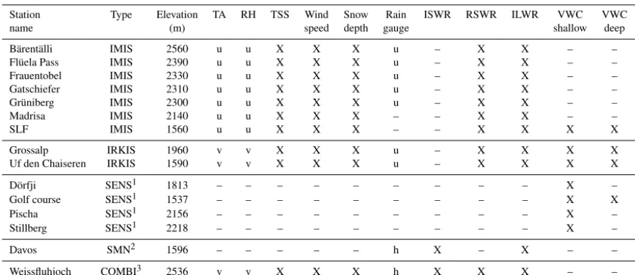
[image:4.612.48.550.105.491.2]

(5)

main-Table 2.List of stations and measured quantities at the stations that are used in this study. “X” indicates measured and used in this study; “–” indicates not measured; “u” indicates unventilated (temperature) or unheated (rain gauge); “v” indicates ventilated; “h” indicates heated rain gauge. Volumetric water content (VWC) shallow denotes soil moisture sensors at 10, 30 and 50 cm depths; VWC deep denotes soil moisture sensors at 80 and 120 cm depths. TA indicates air temperature, RH indicates relative humidity, TSS indicates surface temperatures, ISWR indicates incoming short-wave radiation, RSWR indicates reflected short-wave radiation and ILWR indicates incoming long-wave radiation.

Station Type Elevation TA RH TSS Wind Snow Rain ISWR RSWR ILWR VWC VWC

name (m) speed depth gauge shallow deep

Bärentälli IMIS 2560 u u X X X u – X X – –

Flüela Pass IMIS 2390 u u X X X u – X X – –

Frauentobel IMIS 2330 u u X X X u – X X – –

Gatschiefer IMIS 2310 u u X X X u – X X – –

Grüniberg IMIS 2300 u u X X X u – X X – –

Madrisa IMIS 2140 u u X X X – – X X – –

SLF IMIS 1560 u u X X X – – X X X X

Grossalp IRKIS 1960 v v X X X u – X X X X

Uf den Chaiseren IRKIS 1590 v v X X X u – X X X X

Dörfji SENS1 1813 – – – – – – – – – X –

Golf course SENS1 ₁₅₃₇ _– _– _– _– _– _– _– _– _– _X _X

Pischa SENS1 2156 – – – – – – – – – X –

Stillberg SENS1 2218 – – – – – – – – – X –

Davos SMN2 1596 – – – – – h X – X – –

Weissfluhjoch COMBI3 2536 v v X X X h X X X – –

1_{SENS is a Sensorscope station.}

2_{SMN is a SwissMetNet station (MeteoSwiss).}

3_{COMBI is a combination of IMIS, SwissMetNet and other instrumentation.}

tenance and quality control. One exception is SLF2 in Davos Dorf, which is used as a test station for new sensors or hard-ware. During the winter season of 2011, and for a large part of the winter season of 2012, the relative humidity sensor was providing erroneous data due to a faulty test sensor. The IMIS stations provide a good spatial coverage of the com-mon meteorological parameters, but due to limited energy availability, lack heated rain gauges to assess solid precipita-tion.

In the Davos area, two heated rain gauges are present, located at the SwissMetNet stations WFJ (2536 m a.s.l./2691 m a.s.l.) and Davos Dorf (1590 m a.s.l.), operated by the Swiss Federal Office of Meteorology and Climatology (MeteoSwiss). These stations thereby provide, after applying an undercatch correction, relatively accurate measurements of solid precipitation in winter, in addition to high-quality measurements of common meteorological parameters. For example, these stations also provide incom-ing short-wave and long-wave radiation usincom-ing ventilated and heated sensors to prevent riming and snow covering up the sensors. At WFJ, short-wave and long-wave radiation sensors located at a local mountain peak of 2691 m a.s.l. were used in this study. These sensors experience almost no shadowing from surrounding mountain peaks. The WFJ measurement site at 2536 m a.s.l. is equipped with ventilated temperature and relative humidity sensors. Moreover, several backup sensors are present, allowing for filling data gaps.

The Interkantonales Mess- und Informationssystem (IRKIS) and SensorScope stations were temporarily set up

for this study. IRKIS stations are based on the IMIS design but with a sensor height of 4.5 m. SensorScope stations (In-gelrest et al., 2010) were installed in less accessible terrain to increase quantity and area covered by measurements. Oper-ation of these type of stOper-ations in the harsh winter conditions appeared to be more difficult than expected and the some-times hazardous locations of the measurement sites were hin-dering maintenance during the winter season. Due to sev-eral outages of the stations and broken sensors, the meteo-rological measurement series contain many gaps and are not used as input in this study. The IRKIS and SensorScope sta-tions were additionally equipped with soil moisture sensors at 10, 30 and 50 cm depths. At IRKIS stations and the golf course SensorScope station, soil moisture sensors were also installed at 80 and 120 cm depths. This is schematically il-lustrated in Fig. 3. At each depth, two sensors, labelled “(A)” and “(B)” here, were installed at approximately 50 cm dis-tance. The IRKIS station SLF2 was using the IMIS station SLF2, but soil moisture sensors were installed in close vicin-ity. IRKIS stations report weather and soil moisture condi-tions at a time resolution of 10 min. SensorScope stacondi-tions measure at a time resolution of 1 min, sending their data us-ing GPRS cell phone networks.

[image:5.612.72.526.130.326.2]

(6)

Still-Figure 3.Soil layering as used in the Alpine3D model. The three water fluxes used to drive the hydrologic response model are shown in blue arrows. The soil moisture measurements are indicated by brown circles. The grey area is denoting the part of the soil where the initial soil saturation at the onset of rainfall or snowmelt events was determined.

berg stations were located in the “mixed forest”, “bush” and “bare soil” classes, respectively, which are found in 12.9, 7.3 and 6.0 % of the Dischma catchment, respectively. The SLF2 and golf course stations would officially fall into the category of “settlement”, but one would describe the area as “alpine meadow”.

At the soil moisture measurement sites, Decagon 10HS soil moisture sensors were installed, which have a volume of influence of 1320 mL, or a volume of approximately 11×

[image:6.612.105.229.66.267.2]

11×11 cm (Decagon Devices, 2014). Mittelbach et al. (2012) present an in-depth comparison with other types of soil mois-ture sensors. A few important issues related to the Decagon 10HS sensors that are relevant for this study were reported. In their study, the liquid water content values from the sen-sors exhibited a soil temperature dependency. The sensen-sors were also found to hardly register values above 0.40 m3m−3 and it was concluded that the 10HS shows a decreased sensi-tivity with increasing liquid water content. Consequently, the sensors were unable to follow fluctuations in wet soil con-ditions. For some of the sites and depths where we installed these type of sensors, the measured volumetric water con-tent (VWC) is around or above 0.40 m3m−3. We therefore expect a strongly reduced dynamic response in these loca-tions. However, many of the installed sensors were recording values well below 0.40 m3m−3and provide useful measure-ments. The dielectric constant of ice is much lower than for water, making the sensors mostly sensible to the liquid water content part only.

Table 3.Land use classes and corresponding soil initialisations.

Land use class Area (%) Soil 0–60 cm Soil 60–300 cm

Rock 29.2 loamy sand loamy sand

Alpine meadow 21.1 silt loam sandy loam Rough pasture 15.5 silt loam sandy loam Mixed forest 12.9 silt loam sandy loam

Bush 7.3 silt loam sandy loam

Bare soil 6.0 silt loam sandy loam

Glacier, ice, firn 3.2 ice ice

Pasture 2.6 silt loam sandy loam

Water 1.0 water water

Settlements 0.8 rock rock

Road 0.5 rock rock

Wetland 0.1 silt loam sandy loam

Vegetables <0.1 silt loam sandy loam

3 Methods

3.1 Simulation set-up

SNOWPACK is a one-dimensional, physics-based multilayer snow cover model (Lehning et al., 2002a, b), which provides the surface scheme for Alpine3D. The Richards equation (Richards, 1931) is used to describe soil moisture dynam-ics and is numerically solved using finite differences scheme over the model layers (elements). Water flow in snow is solved by the bucket scheme, which provides accurate snow-pack runoff estimations on daily and seasonal timescales (Wever et al., 2014b), and has noticeably lower computa-tional costs (on the order of a factor of 2–3) than using the full Richards equation for snow. The liquid water outflow from the snowpack is prescribed as the upper boundary con-dition for the Richards equation for the soil (Wever et al., 2014b). In snow-free conditions, the upper boundary condi-tion is defined by rainfall; evaporacondi-tion and deposicondi-tion result from the latent heat flux. Phase changes in soil are calculated following Wever et al. (2015). Water retention curves in the SNOWPACK model are based on the van Genuchten model (van Genuchten, 1980) via predefined soil types as in the ROSETTA class average parameters (Schaap et al., 2001).

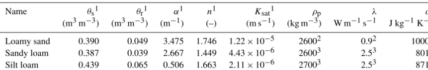
[image:6.612.311.543.86.243.2]

(7)

calcu-Table 4.List of parameters for the soil types for saturated water content (θs), residual water content (θr), the van Genuchten parametersα

andn, the saturated hydraulic conductivity (Ksat(1)), the density of soil particles (ρp), the thermal conductivity of soil particles (λ) and the

specific heat of soil particles (cp).

Name θs1 θr1 α1 n1 Ksat1 ρp λ cp

(m3m−3) (m3m−3) (m−1) (–) (m s−1) (kg m−3) W m−1s−1 J kg−1K−1

Loamy sand 0.390 0.049 3.475 1.746 1.22×10−5 26002 0.92 10002

Sandy loam 0.387 0.039 2.667 1.449 4.43×10−6 26003 2.53 8013

Silt loam 0.439 0.065 0.506 1.663 2.11×10−6 27003 2.53 8713

1_{ROSETTA class average parameters (Schaap et al., 2001).}2_{Bachmann et al. (2001).}3_{Ochsner et al. (2001).}

lation of the wind fields and snow drift poses a high computa-tional demand compared to the other modules. The different modules and the coupling strategy are described in Lehning et al. (2006).

The Alpine3D simulations were run for a domain of 21.5 km×21.5 km with a grid cell size of 100 m×100 m, giv-ing a total size of 215×215 grid cells. The model was run in hourly time steps, providing meteorological forcing data per time step for each pixel by interpolating from the meteoro-logical stations in and just outside the Davos area using the MeteoIO library (Bavay and Egger, 2014). Per hourly time step, four SNOWPACK time steps are executed at 15 min resolution.

At each Alpine3D model time step, the precipitation mea-surements from the heated rain gauges in Davos and WFJ were interpolated over the grid by using the elevation gra-dient from the measurements. The commonly used tempera-ture threshold in the SNOWPACK model of 1.2◦C was used to separate precipitation into rain and snowfall. Air temper-ature, relative humidity and wind speed were also interpo-lated over the grid, using the station data as indicated in Ta-ble 2 and applying an inverse distance weighting interpola-tion with lapse rates calculated from the available data. Only IMIS stations were used for spatial interpolations, except for the radiation components. Incoming long-wave radiation was interpolated using a lapse rate between both SwissMet-Net stations providing radiation. Short-wave radiation is pro-vided by the radiation module, using the measurements from WFJ. The radiation balance is closed by the SNOWPACK simulations at each grid point when SNOWPACK calculates the surface temperature and surface albedo.

Two important components to initialise Alpine3D simula-tions are the digital elevation model (DEM) and distributed soil information. For the Davos area, the DEM is provided by the Swiss Federal Office of Topography (swisstopo). Soil properties were based on the land use classification, as pro-vided by swisstopo (Zappa et al., 2003). Table 3 lists the land use classes, the percentage of areal coverage in the simu-lated area and the soil properties. Pixels that were defined as glacier, ice, firn, road, settlements, rivers and lakes (6 %) were initialised in a state that represents the land use class. Other vegetation-free areas are classified as rocky surface.

This class is assigned to 29 % of the pixels and consists mostly of ground moraine and scree slopes, whereas solid rock and rock walls are sparse in the Davos area. The rocky surface pixels were initialised uniformly with loamy sand. This is based on observations when installing soil tempera-ture sensors at the WFJ, which is located in the rock class and for which plausible simulations were obtained using this soil class (Wever et al., 2015). All other pixels (65 %), in-cluding forests, meadows, pasture, bare soil and occasional pixels that are defined as agricultural use were initialised us-ing an upper layer of 60 cm consistus-ing of silt loam and a lower layer of 240 cm consisting of sandy loam. This choice is based on observations when installing the soil moisture sensors at the IRKIS and SensorScope stations. The soil per-meability classification provided by the Swiss Federal Office for Agriculture (FOAG) shows generally high permeability in the area surrounding Davos, which confirms the choice for soil types with no clay content. To determine thermal prop-erties of the soil, literature values were taken (Table 4). For thermal conductivity, a wide range of values is reported and a strong dependence on water content is present. We used val-ues corresponding to typical soil saturation valval-ues, based on work by Ochsner et al. (2001) and Bachmann et al. (2001). The skeleton fraction of the soil is largely unknown, and al-though it may impact the soil hydraulic properties signifi-cantly (Brakensiek and Rawls, 1994) and thereby soil mois-ture and streamflow simulations (Rössler and Löffler, 2010), the SNOWPACK model currently does not support pedo-transfer functions that take the skeleton fraction into account, and hence it was neglected in our simulations.

A soil depth of 3 m was simulated, subdivided into 23 lay-ers, as illustrated in Fig. 3. The layer spacing was 2 cm near the surface, increasing to 25 cm at 3 m depth. The densely spaced surface layers are necessary to describe the large gra-dients of temperature and moisture occurring in this region. The lower boundary condition at 3 m depth was set as a water table condition for the liquid water flow and as a constant up-ward geothermal heat flux of 0.06 W m−2for the heat equa-tion.

[image:7.612.85.516.109.180.2]

(8)

roughness length during the presence of a snow cover was defined to be 0.015 m below 1900 m a.s.l. and 0.002 m other-wise. This division is based on the generally rougher terrain below 1900 m, due to the presence of trees or large bushes, whereas above 1900 m, mainly meadows and scree fields are present. When pixels are snow free, they were assigned a roughness length of 0.02 m.

Alpine3D has recently been extended with support for the parallelisation protocol MPI, allowing for the parallelisation of the distributed SNOWPACK and energy balance simula-tions. Using 36 CPU cores from a HPC system consisting of a total of 32 compute nodes with two six-core AMD Opteron 2439 2.8 GHz processors per compute node, the computa-tion took on average 14 h of wall clock time for a single year, mainly depending on the snow depth in the winter season.

3.2 Analysis

The soil moisture measurements series were first cleaned for erroneous data, like negative values, or data from broken sen-sors after visual inspection of the time series. Then, data were aggregated to hourly and daily timescales by calculating av-erage soil moisture contents over the respective time spans. From the simulations, the modelled soil moisture values were extracted for each depth at which measurements were taken. The output resolution was 1 h and daily values were calcu-lated by averaging the hourly values.

As the area of Davos is dominated by snowfall in winter, a separation is made for yearly, summer and winter periods. The summer months are defined as the period from June to October. At the elevation of the soil moisture stations, snow-fall episodes are almost absent in these months and the winter snow cover has melted completely by the beginning of June. The winter months are defined as the period from November to May, when a snow cover is present. Note that, typically, the snow cover melts away in April or May at the stations, and in those months the soil moisture is expected to be strongly influenced by the snowmelt from the snowpack.

The streamflow from the Dischmabach is calculated using a spatially explicit and semi-distributed hydrologic response model that casts the soil moisture dynamics in a travel time distribution framework (Comola et al., 2015b; Gallice et al., 2016). Specifically, the model simulates hydrologic transport within subcatchment soil compartments and the stream net-work, identified through geomorphological analysis of the digital elevation model (Tarboton, 1997). An upper soil com-partment is recharged by a water flux provided by the surface scheme of the Alpine3D model. Part of the outflow from the upper soil compartment generates interflow, which represents the fast hydrologic response. The remaining part recharges a lower soil compartment, where the slow groundwater flow in generated. However, it is a priori not clear where to draw the boundary between the surface scheme and the hydrologic response model. To investigate this, we tested three scenar-ios by using the soil water flux at 2, 30 and 60 cm depths (see

Fig. 3). This approach allows the Alpine3D model to run with a thick soil layer (3 m), easing the choice of lower boundary condition for the soil (geothermal heat flux and a water ta-ble). The 2 cm flux represents a case where almost all water input into the soil from both snowmelt as well as rainfall is directly routed using the hydrologic response model, while at the same time ensuring that evaporation is taken into account. It basically represents the case where soil is neglected for the discharge simulations. The simulations using the flux at 30 or 60 cm depths are performed to verify the sensitivity of the hydrologic response model to the thickness of the soil lay-ers used in Alpine3D. The water flux at all grid points whose centre point is inside the polygons of the 55 subcatchments is summed and provided to the hydrologic response model. The subcatchments are determined by analysing the digital elevation model (Comola et al., 2015b).

It is noteworthy that the hydrological model is parsimo-nious in terms of calibration parameters due to the explicit analysis of the catchment’s geomorphological complexity and the physically based simulation of surface processes pro-vided by Alpine3D. In particular, the two compartments and the recharge rate in the travel time distribution approach of the hydrologic response model give three parameters that re-quire calibration: the average travel time of the upper and lower soil compartments (day) and the maximum recharge rate of the lower compartment from the upper compartment (mm day−1). Here, all three approaches which define the input for the hydrologic response model are independently calibrated with measured discharge from October 2004 to September 2009 using Monte Carlo simulations with 5000 repetitions. The best combination of coefficients was deter-mined based on the highest Nash–Sutcliffe model efficiency (NSE) coefficient (Nash and Sutcliffe, 1970). The period from October 2009 to September 2014 was used for valida-tion.

(9)

0 50 100 150 200 250 300

10 11 12 1 2 3 4 5 6

(2011)7 8 9 10 11 12 1 2 3 4 5 (2012)6 7 8 9 10 11 12 1 2 3 4 5 (2013)6 7 8 9

Snow depth (cm)

Month

Measured Simulated Grossalp

(c)

0 50 100 150 200 250

10 11 12 1 2 3 4 5 6 (2011)

7 8 9 10 11 12 1 2 3 4 5 6 (2012)

7 8 9 10 11 12 1 2 3 4 5 6 (2013)

7 8 9

Snow depth (cm)

Month

Measured Simulated Uf den Chaiseren

(b)

0 50 100 150 200

10 11 12 1 2 3 4 5 6 (2011)

7 8 9 10 11 12 1 2 3 4 5 6 (2012)

7 8 9 10 11 12 1 2 3 4 5 6 (2013)

7 8 9 10

Snow depth (cm)

Month

Measured Simulated SLF2

[image:9.612.98.497.68.366.2]

(a)

Figure 4.Measured and simulated snow depth for stations SLF2(a), Uf den Chaiseren(b)and Grossalp(c)for the period October 2010 to October 2013. Noisy signals in the summer months arise from grass growth below the sensor.

excluding the summer season, showing that these events are concentrated in the spring season.

4 Results and discussion

4.1 Snow height

Figure 4 shows measured and simulated snow depth by Alpine3D for stations SLF2, Uf den Chaiseren and Grossalp. In snow seasons 2011 and 2013, the snow depth in the Alpine3D simulations is satisfyingly reproduced at both SLF2 and Uf den Chaiseren. The snow depth at Grossalp is overestimated in all snow seasons. This is explained by the fact that this particular site is relatively sensitive to wind eroding snow from the surface. The snow depth in the snow season of 2012 is overestimated at all stations, which is re-lated to unusual meteorological circumstances of large snow-fall accompanied by strong winds, which lead to an overesti-mation of precipitation as measured by the heated rain gauge (also discussed in Wever et al., 2015). Nevertheless, the snow cover development at those three sites is overall satisfactorily simulated in Alpine3D for providing an upper boundary for the soil. In the summer months, grass growth below the sen-sor is visible as an increase in snow depth with a highly noisy

signal. Mowing activity is indicated by sudden decreases in snow depth.

4.2 Soil moisture

(10)

0 0.1 0.2 0.3 0.4 0.5

10 11 12 1 2 3 4 5 6

(2011)7 8 9 10 11 12 1 2 3 4 (2012)5 6 7 8 9 10 11 12 1 2 3 4 5 (2013)6 7 8 9 10 0 50 100 150 200 250 V o lu m e tr ic c o n te n t (c m c m ) 3 -3

Snow depth (cm)

Month Simulated: 10 cm (water)

Simulated: 10 cm (ice)

Measured: 10 cm (A) Measured: 10 cm (B)

Simulated snow depth

0 0.1 0.2 0.3 0.4 0.5

10 11 12 1 2 3 4 5 6 (2011)

7 8 9 10 11 12 1 2 3 4 5 6 (2012)

7 8 9 10 11 12 1 2 3 4 5 6 (2013)

7 8 9 10 0 0.1 0.2 0.3 0.4 0.5 V o lu m e tr ic c o n te n t (c m c m ) 3 -3

Snow depth (cm)

Simulated: 30 cm (ice) Measured: 30 cm (A)Measured: 30 cm (B)

0 0.1 0.2 0.3 0.4 0.5

10 11 12 1 2 3 4 5 6 (2011)

7 8 9 10 11 12 1 2 3 4 5 6 (2012)

7 8 9 10 11 12 1 2 3 4 5 6 (2013)

Snow depth (cm)

0 0.1 0.2 0.3 0.4 0.5

10 11 12 1 2 3 4 5 6

(2011)7 8 9 10 11 12 1 2 3 4 (2012)5 6 7 8 9 10 11 12 1 2 3 4 5 (2013)6 7 8 9 10 0 0.1 0.2 0.3 0.4 0.5 V o lu m e tr ic c o n te n t (c m c m ) 3 -3

Snow depth (cm)

0 0.1 0.2 0.3 0.4 0.5

10 11 12 1 2 3 4 5 6 (2011)

7 8 9 10 11 12 1 2 3 4 5 6 (2012)

7 8 9 10 11 12 1 2 3 4 5 6 (2013)

Snow depth (cm)

[image:10.612.96.495.64.533.2]

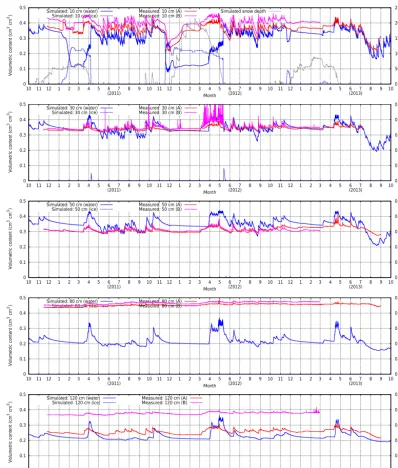
Figure 5.Measured and simulated soil moisture at the IRKIS station SLF2, for (from top to bottom) 10, 30, 50, 80 and 120 cm depths for the period October 2010 to October 2013. In the upper panel, simulated snow depth is also shown.

tion. A detailed example hereof is shown in Fig. 7c, d for the snow-free month of June 2011 for the SLF2 measure-ment site. Particularly large rainfall events are strongly in-fluencing soil moisture, compared to small ones. Generally, the simulated soil moisture reacts more strongly to incoming rainwater and also shows stronger fluctuations on subdaily timescales than in the measurements.

At several stations, soil freezing is indicated by the soil moisture sensors. Significant soil freezing was occurring in the snow season of 2011, as clearly visible at SLF2 (Fig. 5) and Uf den Chaiseren (Fig. 6), as well as at Stillberg (see

(11)

0 0.1 0.2 0.3 0.4 0.5

11 12 1 2 3 4 5 6 (2011)

7 8 9 10 11 12 1 2 3 4 5 6 (2012)

7 8 9 10 11 12 1 2 3 4 5 6 (2013)

7 8 9 0 50 100 150 200 250

Snow depth (cm)

Simulated snow depth

0 0.1 0.2 0.3 0.4 0.5

11 12 1 2 3 4 5 6

(2011)7 8 9 10 11 12 1 2 3 4 (2012)5 6 7 8 9 10 11 12 1 2 3 4 (2013)5 6 7 8 9 0 0.1 0.2 0.3 0.4 0.5

Snow depth (cm)

0 0.1 0.2 0.3 0.4 0.5

11 12 1 2 3 4 5 6 (2011)

7 8 9 10 11 12 1 2 3 4 5 6 (2012)

7 8 9 10 11 12 1 2 3 4 5 6 (2013)

7 8 9 0 0.1 0.2 0.3 0.4 0.5

Snow depth (cm)

0 0.1 0.2 0.3 0.4 0.5

11 12 1 2 3 4 5 6

(2011)7 8 9 10 11 12 1 2 3 4 (2012)5 6 7 8 9 10 11 12 1 2 3 4 (2013)5 6 7 8 9 0 0.1 0.2 0.3 0.4 0.5

Snow depth (cm)

0 0.1 0.2 0.3 0.4 0.5

11 12 1 2 3 4 5 6 (2011)

7 8 9 10 11 12 1 2 3 4 5 6 (2012)

7 8 9 10 11 12 1 2 3 4 5 6 (2013)

7 8 9 0 0.1 0.2 0.3 0.4 0.5

Snow depth (cm)

[image:11.612.98.494.65.532.2]

V o lu m e tr ic c o n te n t (c m c m ) 3 -3 V o lu m e tr ic c o n te n t (c m c m ) 3 -3 V o lu m e tr ic c o n te n t (c m c m ) 3 -3 V o lu m e tr ic c o n te n t (c m c m ) 3 -3 V o lu m e tr ic c o n te n t (c m c m ) 3 -3

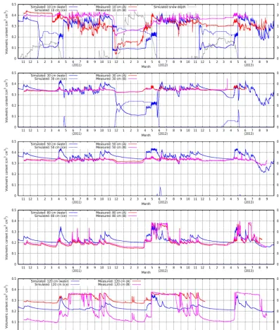
Figure 6.Measured and simulated soil moisture at the IRKIS station Uf den Chaiseren, for (from top to bottom) 10, 30, 50, 80 and 120 cm depths for the period October 2010 to October 2013. In the upper panel, simulated snow depth is also shown.

The simulations show soil freezing at 10 cm depth in all snow seasons at most stations, for at least a short period of time, which is more soil freezing than captured in the soil moisture measurements. The overestimation of soil freezing in the simulations may be partly related to neglecting the presence of vegetation at the measurement sites. All sites are covered by grass or rough pasture and bushes. To account for the insulating effects of the canopy, some soil freezing schemes consider the presence of a canopy when calculating soil phase changes (e.g. Giard and Bazile, 2000). Due to the lack of possible validation data, we did not implement this.

(12)

0 0.1 0.2 0.3 0.4 0.5

01−03 04−03 07−03 10−03 13−03 16−03 19−03 22−03 25−03 28−03 31−03 30 35 40 45 50 55 60 65 70 V o lu m e tr ic c o n te n t (c m c m ) 3 -3

Snow depth (cm)

Date (2011) A3D: 10 cm (water)

A3D: 10 cm (ice)

MSR: 10 cm (A) MSR: 10 cm (B)

Snow depth (A3D)

(a) 0 0.1 0.2 0.3 0.4 0.5

01−03 04−03 07−03 10−03 13−03 16−03 19−03 22−03 25−03 28−03 31−03 0 0.1 0.2 0.3 0.4 0.5 V o lu m e tr ic c o n te n t (c m c m ) 3 -3

Snow depth (cm)

A3D: 30 cm (ice)

(b) 0 0.1 0.2 0.3 0.4 0.5

01−06 04−06 07−06 10−06 13−06 16−06 19−06 22−06 25−06 28−06 0 2 4 6 8 10 12 V o lu m e tr ic c o n te n t (c m c m ) 3 -3

Snow depth (cm) / Precipitation (mm)

A3D: 10 cm (ice)

Precipitation (c) 0 0.1 0.2 0.3 0.4 0.5

01−06 04−06 07−06 10−06 13−06 16−06 19−06 22−06 25−06 28−06 0 2 4 6 8 10 12 V o lu m e tr ic c o n te n t (c m c m ) 3 -3

Snow depth (cm) / Precipitation (mm)

A3D: 30 cm (ice)

[image:12.612.100.494.67.252.2]

(d)

Figure 7.Measured (MSR) and simulated (A3D) soil moisture at the IRKIS station SLF2, for 10 cm depth(a, c)and 30 cm depth(b, d),

during the snowmelt season(a, b)and a snow-free summer month(c, d). Panel(a)additionally shows simulated snow depth and panel(c)

additionally shows precipitation.

ple, for some sites we get an adequate soil moisture simu-lation without considering the skeleton fraction, whereas for other sites the simulations are showing less agreement with measurements. This would then only allow for an ad hoc modification of the skeleton fraction, as we cannot separate well enough between the soil moisture sites based on avail-able information (land use and soil permeability).

The relatively dry summer of 2013, most pronounced at low elevations as indicated by the difference in summer pre-cipitation from both heated rain gauges (Table 1), is clearly visible in the simulations by a drop in soil moisture at all depths, reaching the lowest values of the entire measurement period. Unfortunately, soil moisture sensors had stopped working at many stations by this time, but at the SLF2 and Stillberg sites, a good correspondence is found in the 10 cm measured and simulated soil moisture series. At the Uf den Chaiseren site, the recession curve during this summer is par-ticularly present at the sensors at 50 and 80 cm depths, and absent in the highest sensor.

Some features are found that likely relate to hydrological processes that are not simulated in the Alpine3D model. For example, at the Uf den Chaiseren site, the soil moisture at 80 and 120 cm is clearly influenced by a rising water table in the late snowmelt season. This is indicated by the sudden rise to high values of saturation, remaining constant after-wards (Fig. 6). The soil at the golf course station appeared to be close to saturation for extended periods of time (see Fig. S5 in the Supplement), which is congruent with observa-tions when installing the sensors. The location of these two stations close to the Dischmabach (Uf den Chaiseren) and Landwasser river (golf course station), which are partly fed by meltwater from the glacierised area, supports this inter-pretation. The apparent interaction with groundwater levels

at these stations is not considered in the simulations, as the groundwater table is fixed at the lower boundary of the soil column in the model domain. Similarly, the measurements at 10 and 30 cm depths at the Grossalp station (see Fig. S1 in the Supplement) also indicate high saturation of the soil, for which no source of water could be found. Due to the insensitivity of the soil moisture sensors in wet soil condi-tions, discrepancies between simulations and measurements as found at the Grossalp and golf course stations can only be assessed qualitatively and provide insights on the limitations of the measurements and simulations. In contrast with the other measurement sites, the soil moisture sensors at the Pis-cha station show a very dynamic response (see Fig. S3 in the Supplement). We cannot exclude that during the installation of the sensors, the soil was disturbed in such a way that af-terwards, efficient preferential flow paths occurred along the boundaries of the displaced soil layers.

Figure 8 shows ther2values between daily averaged mea-sured and simulated soil moisture values for the various depths for the full period and for the summer months only. Here, soil moisture was taken as the sum of ice and wa-ter to compensate for the overestimation of soil freezing. Only the values for the sensor with the highestr2 value of the two sensors per depth are shown. Generally, the highest

(13)

0 0.2 0.4 0.6 0.8 1

Stillberg Dorfji Pischa Golf

courseGrossalp Uf denChaiserenSLF2

r

2

station

10 cm Avg. (0.21) 30 cm Avg. (0.27) 50 cm Avg. (0.40) 80 cm Avg. (0.10) 120 cm Avg. (0.14)

(a)

0 0.2 0.4 0.6 0.8 1

Stillberg Dorfji Pischa Golf

courseGrossalp Uf denChaiserenSLF2

r

2

station

10 cm Avg. (0.34) 30 cm Avg. (0.36) 50 cm Avg. (0.41) 80 cm Avg. (0.09) 120 cm Avg. (0.15)

[image:13.612.102.492.66.186.2]

(b)

Figure 8.Ther2values between measured and simulated soil moisture for the full period(a)and the summer months(b)for the seven soil moisture stations. Dashed lines indicate the average value determined over all stations.

0 50 100 150 200 250 300 350

Jan 2005 Jan 2006 Jan 2007 Jan 2008 Jan 2009 Jan 2010 Jan 2011 Jan 2012 Jan 2013 Jan 2014

S

tr

e

a

m

fl

o

w

(

m

d

a

y

-1)

3

Date

[image:13.612.100.498.236.341.2]

Measured Simulated using flux at 2 cm depth Simulated using flux at 30 cm depth Simulated using flux at 60 cm depth Calibration Validation

Figure 9.Measured and simulated daily streamflow for the outlet of the Dischmabach. Dashed lines denote the calibration period; solid lines

denote the validation period. Major ticks on thexaxis are drawn at 1 January of each year; minor ticks are drawn at every other first of the

month.

in the model than the onset of snowpack runoff which deter-mines soil moisture fluctuations in large periods of the year. For deeper layers, the model performance is comparable to the performance for the full year.

The r2 values indicate that, for many sites, some of the variability in soil moisture is adequately captured. This spa-tially varying reproducibility of soil moisture is a typical re-sult for physics-based soil models applied in alpine terrain as, for example, found also by Rössler and Löffler (2010), Ku-mar et al. (2013) and Pasolli et al. (2013). Better agreement (r2 between 0.8 and 0.95) may be achieved by calibrating the water retention curves, or related soil parameters, to the soil moisture measurements (Gurtz et al., 2003; Brocca et al., 2013; Pellet et al., 2016), although the lack of distributed soil information would make a distribution of this calibration over the model domain difficult and not very meaningful.

4.3 Streamflow

Figure 9 shows the measured and simulated streamflow at the outlet of the Dischmabach in the Dischma catchment. The winter periods are clearly identifiable by the hydro-graph falling back to baseflow. Furthermore, high discharge is particularly found in spring, during the snowmelt season which typically lasts from April to June in the Dischma catchment (Griessinger et al., 2016). During the summer

pe-riod, streamflow slowly decreases, interrupted regularly with peaks in streamflow due to rainfall. These general discharge patterns are well captured in the simulations, regardless of the depth below the surface where the liquid water flux is routed to the runoff model. However, the fast dynamics on daily timescales in the Dischmabach streamflow is underes-timated in the simulations, particularly when using the flux at 60 cm depth, for which the deep soil layer apparently has a too strong dampening of the incoming water in order to reproduce daily streamflow behaviour. Improvements in re-producing the dynamic response on short timescales in the simulations could probably be obtained by including lateral water transport in Alpine3D, which would allow to account for the fast surface runoff which, for example, takes place over highly saturated or impervious soils.

(14)

up-dated soil module of SNOWPACK enables a good prediction of streamflow in the summer months. Interpreting the flux at 2 cm depth as the effect of routing snowpack runoff and rain-fall minus evaporation to the hydrologic response model, it shows that including 30 cm of soil layers improves the dis-charge simulation.

We hypothesise that in the Dischma catchment, the snowmelt season is providing large water fluxes from the snow to the soil, compared to the soil water dynamics, mak-ing it the dominant factor in predictmak-ing streamflow. In the summer months, however, the predisposition of the soil is also an important factor, thus neglecting the soil layers al-most completely by routing the 2 cm flux to the runoff model, reducing the model efficiency. The improved results of the 30 cm soil simulations as opposed to using much deeper soils suggests that the temporal dynamics of near-surface water fluxes exert a relevant control on the hydrologic response of these alpine catchments.

4.4 Predisposition from soil moisture

The soil moisture state of the Dischma catchment is sum-marised as the basin-wide average saturation in the upper 40 cm of the soil at the onset of a rainfall or snowpack runoff event. The water flux at this depth provided the highest skill in reproducing observed discharge after applying the hydro-logic response model. Figure 11a shows the runoff coeffi-cient (i.e. the ratio of rainfall to discharge) for the cumulative rainfall and measured discharge from the Dischma catchment as a function of catchment average soil saturation. The figure illustrates that the reduced storage capacity in wetter soils leads indeed to more of the precipitation water being routed to discharge and vice versa. In Fig. 11b, it is illustrated that similar behaviour is also captured in the simulated discharge. For the Dischma catchment, we found that not only the total event runoff coefficient is determined by the soil moisture state but also the peak runoff coefficient, defined as the ratio of the maximum peak in precipitation over the maximum, not necessarily simultaneous, discharge peak (see Fig. 11c for measured discharge). This relationship is again also found for the simulated discharge (Fig. 11d). Although the initial soil moisture impacts the runoff coefficient for both the cu-mulative amounts as well as the peak values, the time lag between a peak in rainfall and measured discharge is not de-pendent on the soil moisture conditions (Fig. 11e). Also, this result is reproduced by the simulated discharge (see Fig. 11f). Allr2values reported in Fig. 11 test significant at the 95 % confidence level.

When the catchment is snow-covered, the meltwater out-flow from the snowpack can be considered analogous to rain-fall in summer. A similar analysis as presented in Fig. 11 is performed using snowpack runoff (see Fig. 12). Also here, we find that the soil moisture state at the onset of snow-pack runoff events influences the streamflow discharge. Sim-ilar to rainfall events, the soil moisture state influences the

ratio of the cumulative measured event discharge over cu-mulative snowpack runoff (Fig. 12a) as well as the peak ratio (Fig. 12c). The correlation coefficients are higher for the snowpack runoff events than for the rainfall events. This higher correlation coefficient for snowpack runoff than for rainfall is also found for the runoff coefficients using simu-lated discharge (Fig. 12b and d). Similar to rainfall events, the time delay between peaks in snowpack runoff and dis-charge is independent of the initial soil moisture state.

In line with previous studies (Maurer and Lettenmaier, 2003; Berg and Mulroy, 2006; Seyfried et al., 2009; Koster et al., 2010), the results confirm that the simulations of the soil moisture state contribute to the understanding of how rainfall and snowpack runoff input in the hydrological system is influencing discharge from the catchment. Based on mea-surements, this relationship was found for alpine catchments for summer rainfall (Penna et al., 2011). However, we show that this effect is reproduced in both measured runoff coef-ficients as well as simulated ones and also exists for snow-pack runoff. The relationship between the initial soil mois-ture state and runoff coefficients is similar for observed and simulated discharge as well as for rainfall or snowpack runoff events. These results suggest that simulations of soil moisture in snow-dominated catchments using the Alpine3D model combined with the hydrologic response model are able to provide understanding of the discharge behaviour from the catchment. Assessing the soil moisture state through such simulations may then help in assessing flood risk.

5 Conclusions

Simulations with the spatially explicit Alpine3D model were performed for the area of Davos. The recent update of the soil module of SNOWPACK, which provides the surface scheme for the Alpine3D model, shows satisfactory results for simulating soil moisture at seven stations with soil mois-ture measurements in the area around Davos. The compari-son included measurements at 10, 30 and 50 cm depths, and at four stations also at 80 and 120 cm depths. Correlation co-efficients show that, generally, the temporal variability is ad-equately captured. However, often a bias between simulated and measured soil moisture was found, as well as between two sensors at the same site and the same depth.

(15)

0 0.2 0.4 0.6 0.8 1

2005 2006 2007 2008 2009 2010 2011 2012 2013 2014

NSE coefficient

Hydrological year Full year

Average full year: 0.80 Melt season Average melt: 0.72 Summer season Average summer: 0.62

(a)

0 0.2 0.4 0.6 0.8 1

2005 2006 2007 2008 2009 2010 2011 2012 2013 2014

NSE coefficient

(b)

0 0.2 0.4 0.6 0.8 1

2005 2006 2007 2008 2009 2010 2011 2012 2013 2014

NSE coefficient

[image:15.612.100.497.66.169.2]

(c)

Figure 10.NSE coefficients for simulated daily streamflow for the outlet of the Dischmabach, using the 2 cm(a), 30 cm(b)or 60 cm(c)

water fluxes in the soil layers.

ﬀ

ﬃ

≥

ﬀ

ﬃ

≥

ﬀ

ﬃ

≥

ﬀ

ﬃ

≥

ﬀ

≥

ﬀ

≥ ( )

( ) ( )

( )

( ) ( )

Figure 11.Rainfall event runoff coefficients for measured discharge as a function of initial soil saturation in the upper 40 cm of the soil(a)

and similar results for simulated discharge(b). Peak rainfall runoff coefficients for measured discharge as a function of soil saturation(c)

and similar results for simulated discharge(d). Time difference between peak rainfall and measured peak discharge(e)and similar results

[image:15.612.129.468.217.639.2]

(16)

ﬀ

ﬃ

≥

ﬀ

ﬃ

≥

ﬀ

ﬃ

≥

ﬀ

ﬃ

≥

ﬀ

≥

ﬀ

≥

ﬀ

( )

( ) ( )

( )

[image:16.612.131.467.65.485.2]

( ) ( )

Figure 12.Snowpack runoff event runoff coefficients for measured discharge as a function of initial soil saturation in the upper 40 cm of

the soil(a)and similar results for simulated discharge(b). Peak snowpack runoff coefficients for measured discharge as a function of soil

saturation(c)and similar results for simulated discharge(d). Time difference between peak snowpack runoff and measured peak discharge

(e)and similar results for simulated peak discharge. Points are coloured according to the event snowpack runoff sum(a, b)or the peak

snowpack runoff(c, d, e, f).

Relating the water flux at 30 cm depth in the soil to stream-flow in the Dischma catchment using a travel time distribu-tion approach provided a higher agreement with observed streamflow than directly using the water flux at the top of the soil or at 60 cm depth. This may be a result of the (on av-erage) relatively shallow layer of soil, which influences the near-surface water dynamics in alpine terrain and is impor-tant to consider in the simulations. The analysis of events with high rainfall or snowpack runoff with return periods of approximately 15 and 30 times per year, respectively, showed that event and peak runoff coefficients using measured dis-charge were found to correlate with the simulated soil

(17)

Code and data availability. The Alpine3D, StreamFlow and SNOWPACK models as well as the MeteoIO prepro-cessing library are available under a LGPLv3 license at http://models.slf.ch. The soil moisture measurements, in situ meteorological measurements from the SensorScope stations, as well as interpolated meteorological model driving data at the soil measurement sites (enabling offline in situ simula-tions) are available at EnviDat (https://doi.org/10.16904/17, Wever, 2017). Measurements from the WFJ measurement site can also be retrieved at Envidat (https://doi.org/10.16904/1, WSL Institute for Snow and Avalanche Research SLF, 2015). Rain gauge data and radiation data from the Davos and the 2691 m Weissfluhjoch site can be accessed via MeteoSwiss (https://gate.meteoswiss.ch/idaweb/). IMIS station data can be requested via http://www.slf.ch/dienstleistungen/daten/index_DE.

The Supplement related to this article is available online at https://doi.org/10.5194/hess-21-4053-2017-supplement.

Competing interests. The authors declare that they have no conflict of interest.

Acknowledgements. This research has been conducted in the

framework of the IRKIS project supported by the Office for Forests and Natural Hazards of the Swiss Canton of Grisons (Christian Wilhelm), the region of South Tyrol (Italy) and the community of Davos. Contributions from the Swiss National Science Foundation (SNF: 200021_150146 and 200021E-160667) are further acknowledged. We also thank Tobias Jonas for installing and maintaining the soil moisture measurements for stations Uf den Chaiseren, Grossalp and SLF2, and S. Valär for kindly allowing the installation of soil moisture sensors and weather stations on his property.

Edited by: Matthias Bernhardt Reviewed by: two anonymous referees

References

Bachmann, J., Horton, R., Ren, T., and van der Ploeg, R. R.: Comparison of the thermal properties of four wettable and four water-repellent soils, Soil Sci. Soc. Am. J., 65, 1675–1679, https://doi.org/10.2136/sssaj2001.1675, 2001.

Bales, R. C., Hopmans, J. W., O’Geen, A. T., Meadows, M., Hart-sough, P. C., Kirchner, P., Hunsaker, C. T., and Beaudette, D.: Soil moisture response to snowmelt and rainfall in a Sierra Nevada mixed-conifer forest, Vadose Zone J., 10, 786–799, https://doi.org/10.2136/vzj2011.0001, 2011.

Bavay, M. and Egger, T.: MeteoIO 2.4.2: a preprocessing library for meteorological data, Geosci. Model Dev., 7, 3135–3151, https://doi.org/10.5194/gmd-7-3135-2014, 2014.

Bavay, M., Lehning, M., Jonas, T., and Löwe, H.: Simulations of fu-ture snow cover and discharge in Alpine headwater catchments,

Hydrol. Proc., 23, 95–108, https://doi.org/10.1002/hyp.7195, 2009.

Bavay, M., Grünewald, T., and Lehning, M.: Response of snow cover and runoff to climate change in high Alpine catch-ments of Eastern Switzerland, Adv. Water Resour., 55, 4–16, https://doi.org/10.1016/j.advwatres.2012.12.009, 2013. Berg, A. A. and Mulroy, K. A.: Streamflow predictability in the

Saskatchewan/Nelson River basin given macroscale estimates of the initial soil moisture status, Hydrolog. Sci. J., 51, 642–654, https://doi.org/10.1623/hysj.51.4.642, 2006.

Brakensiek, D. and Rawls, W.: Soil containing rock

frag-ments: effects on infiltration, Catena, 23, 99–110,

https://doi.org/10.1016/0341-8162(94)90056-6, 1994.

Brocca, L., Tarpanelli, A., Moramarco, T., Melone, F., Ratto, S., Cauduro, M., Ferraris, S., Berni, N., Ponziani, F., Wagner, W., and Melzer, T.: Soil moisture estimation in alpine catchments through modeling and satellite observations, Vadose Zone J., 12, https://doi.org/10.2136/vzj2012.0102, 2013.

Comola, F., Schaefli, B., Ronco, P. D., Botter, G., Bavay, M., Rinaldo, A., and Lehning, M.: Scale-dependent ef-fects of solar radiation patterns on the snow-dominated hydrologic response, Geophys. Res. Lett., 42, 3895–3902, https://doi.org/10.1002/2015GL064075, 2015a.

Comola, F., Schaefli, B., Rinaldo, A., and Lehning, M.: Thermody-namics in the hydrologic response: Travel time formulation and application to Alpine catchments, Water Resour. Res., 51, 1671– 1687, https://doi.org/10.1002/2014WR016228, 2015b.

Decagon Devices: 10HS soil moisture sensor, Tech.

rep., available at: http://www.decagon.com/en/soils/

volumetric-water-content-sensors/10hs-large-volume-vwc/ (last access: 8 August 2017), 2014.

Federal Office for the Environment (FOEN):

Produktinfor-mation einzugsgebietsgliederung schweiz ezgg-ch, Web

document in German, available at: https://www.bafu.

admin.ch/dam/bafu/de/dokumente/wasser/fachinfo-daten/ produktedokumentationeinzugsgebietsgliederungschweiz.pdf (last access: 8 August 2017), 2015.

Federal Office for the Environment (FOEN): Dischmabach – Davos, Kriegsmatte 2327, available at: https://www.hydrodaten.admin. ch/de/2327.html (retrieved at: 24 May 2017), 2017

Frei, C., Davies, H., Gurtz, J., and Schär, C.: Climate

dynamics and extreme precipitation and flood events

in Central Europe, Integr. Assess., 1, 1389–5176,

https://doi.org/10.1023/A:1018983226334, 2000.

Gallice, A., Bavay, M., Brauchli, T., Comola, F., Lehning, M., and Huwald, H.: StreamFlow 1.0: an extension to the spatially distributed snow model Alpine3D for hydrological modelling and deterministic stream temperature prediction, Geosci. Model Dev., 9, 4491–4519, https://doi.org/10.5194/gmd-9-4491-2016, 2016.

Giard, D. and Bazile, E.: Implementation of a new

assimilation scheme for soil and surface

vari-ables in a global NWP model, Mon. Weather

Rev., 128, 997–1015,

https://doi.org/10.1175/1520-0493(2000)128<0997:IOANAS>2.0.CO;2, 2000.

(18)

SNOWPACK, version 3.2.1, revision 741), Geosci. Model Dev., 8, 2379–2398, https://doi.org/10.5194/gmd-8-2379-2015, 2015. Griessinger, N., Seibert, J., Magnusson, J., and Jonas, T.:

Assess-ing the benefit of snow data assimilation for runoff modelAssess-ing in Alpine catchments, Hydrol. Earth Syst. Sci., 20, 3895–3905, https://doi.org/10.5194/hess-20-3895-2016, 2016.

Groot Zwaaftink, C. D., Cagnati, A., Crepaz, A., Fierz, C., Ma-celloni, G., Valt, M., and Lehning, M.: Event-driven deposi-tion of snow on the Antarctic Plateau: analyzing field mea-surements with SNOWPACK, The Cryosphere, 7, 333–347, https://doi.org/10.5194/tc-7-333-2013, 2013.

Grünewald, T. and Lehning, M.: Are flat-field snow depth measure-ments representative? a comparison of selected index sites with areal snow depth measurements at the small catchment scale, Hy-drol. Proc., 29, 1717–1728, https://doi.org/10.1002/hyp.10295, 2015.

Gurtz, J., Zappa, M., Jasper, K., Lang, H., Verbunt, M., Badoux, A., and Vitvar, T.: A comparative study in modelling runoff and its components in two mountainous catchments, Hydrol. Proc., 17, 297–311, https://doi.org/10.1002/hyp.1125, 2003.

Ingelrest, F., Barrenetxea, G., Schaefer, G., Vetterli, M., Couach, O., and Parlange, M.: SensorScope: Application-specific sensor network for environmental monitoring, ACM Trans. Sens. Netw., 6, https://doi.org/10.1145/1689239.1689247, 2010.

Koster, R. D., Mahanama, S. P. P., Livneh, B., Lettenmaier, D. P., and Reichle, R. H.: Skill in streamflow forecasts derived from large-scale estimates of soil moisture and snow, Nature Geosci., 3, 613–616, https://doi.org/10.1038/ngeo944, 2010.

Kumar, M., Marks, D., Dozier, J., Reba, M., and Winstral, A.: Eval-uation of distributed hydrologic impacts of temperature-index and energy-based snow models, Adv. Water Resour., 56, 77–89, https://doi.org/10.1016/j.advwatres.2013.03.006, 2013. Lehning, M., Bartelt, P., Brown, B., Russi, T., Stöckli, U., and

Zimmerli, M.: SNOWPACK calculations for avalanche warning based upon a new network of weather and snow stations, Cold Reg. Sci. Technol., 30, 145–157, https://doi.org/10.1016/S0165-232X(99)00022-1, 1999.

Lehning, M., Bartelt, P., Brown, B., Fierz, C., and Satyawali, P.: A physical SNOWPACK model for the Swiss avalanche warning Part II: Snow microstructure, Cold Reg. Sci. Technol., 35, 147– 167, https://doi.org/10.1016/S0165-232X(02)00073-3, 2002a. Lehning, M., Bartelt, P., Brown, B., and Fierz, C.: A

phys-ical SNOWPACK model for the Swiss avalanche warn-ing Part III: Meteorological forcwarn-ing, thin layer formation and evaluation, Cold Reg. Sci. Technol., 35, 169–184, https://doi.org/10.1016/S0165-232X(02)00072-1, 2002b. Lehning, M., Völksch, I., Gustafsson, D., Nguyen, T. A., Stähli,

M., and Zappa, M.: ALPINE3D: a detailed model of mountain surface processes and its application to snow hydrology, Hydrol. Proc., 20, 2111–2128, https://doi.org/10.1002/hyp.6204, 2006. Lehning, M., Löwe, H., Ryser, M., and Raderschall, N.:

Inhomogeneous precipitation distribution and snow trans-port in steep terrain, Water Resour. Res., 44, W07404, https://doi.org/10.1029/2007WR006545, 2008.

Marks, D., Link, T., Winstral, A., and Garen, D.:

Simu-lating snowmelt processes during rain-on-snow over a

semi-arid mountain basin, Ann. Glaciol., 32, 195–202,

https://doi.org/10.3189/172756401781819751, 2001.

Maurer, E. P. and Lettenmaier, D. P.: Predictability of seasonal runoff in the Mississippi River basin, J. Geophys. Res., 108, 8607, https://doi.org/10.1029/2002JD002555, 2003.

Mazurkiewicz, A. B., Callery, D. G., and McDonnell, J. J.: Assess-ing the controls of the snow energy balance and water available for runoff in a rain-on-snow environment, J. Hydrol., 354, 1–14, https://doi.org/10.1016/j.jhydrol.2007.12.027, 2008.

McNamara, J. P., Chandler, D., Seyfried, M., and Achet, S.: Soil moisture states, lateral flow, and streamflow generation in a semi-arid, snowmelt-driven catchment, Hydrol. Proc., 19, 4023–4038, https://doi.org/10.1002/hyp.5869, 2005.

Michlmayr, G., Lehning, M., Koboltschnig, G., Holzmann, H., Zappa, M., Mott, R., and Schöner, W.: Application of the Alpine 3D model for glacier mass balance and glacier runoff studies at Goldbergkees, Austria, Hydrol. Proc., 22, 3941–3949, https://doi.org/10.1002/hyp.7102, 2008.

Mittelbach, H., Lehner, I., and Seneviratne, S. I.:, Com-parison of four soil moisture sensor types under field conditions in Switzerland, J. Hydrol., 430–431, 39–49, https://doi.org/10.1016/j.jhydrol.2012.01.041, 2012.

Mott, R., Faure, F., Lehning, M., Löwe, H., Hynek, B., Michlmayer, G., Prokop, A., and Schöner, W.: Simulation of seasonal snow-cover distribution for glacierized sites on Sonnblick, Aus-tria, with the Alpine3D model, Ann. Glaciol., 49, 155–160, https://doi.org/10.3189/172756408787814924, 2008.

Mott, R., Schirmer, M., Bavay, M., Grünewald, T., and Lehning, M.: Understanding snow-transport processes shap-ing the mountain snow-cover, The Cryosphere, 4, 545–559, https://doi.org/10.5194/tc-4-545-2010, 2010.

Nash, J. and Sutcliffe, J.: River flow forecasting through conceptual models part I - A discussion of principles, J. Hydrol., 10, 282– 290, https://doi.org/10.1016/0022-1694(70)90255-6, 1970. Ochsner, T. E., Horton, R., and Ren, T.: A new perspective on

soil thermal properties, Soil Sci. Soc. Am. J., 65, 1641–1647, https://doi.org/10.2136/sssaj2001.1641, 2001.

Pasolli, L., Bertoldi, G., Chiesa, S. D., Niedrist, G., Tappeiner, U., Zebisch, M., and Notarnicola, C.: Multi-source and

multi-scale soil moisture dynamic modelling in

moun-tain meadows, in 2013 IEEE International Geoscience and

Remote Sensing Symposium – IGARSS, pp. 763–766,

https://doi.org/10.1109/IGARSS.2013.6721269, 2013.

Pellet, C., Hilbich, C., Marmy, A., and Hauck, C.: Soil moisture data for the validation of permafrost models using direct and indirect measurement approaches at three alpine sites, Front. Earth Sci., 3, 91, https://doi.org/10.3389/feart.2015.00091, 2016.

Penna, D., Tromp-van Meerveld, H. J., Gobbi, A., Borga, M., and Dalla Fontana, G.: The influence of soil mois-ture on threshold runoff generation processes in an alpine headwater catchment, Hydrol. Earth Syst. Sci., 15, 689–702, https://doi.org/10.5194/hess-15-689-2011, 2011.

Richards, L.: Capillary conduction of liquids through

porous mediums, J. Appl. Phys., 1, 318–333,

https://doi.org/10.1063/1.1745010, 1931.

Rigon, R., Bertoldi, G., and Over, T. M.: GEOtop: A distributed hydrological model with coupled water and energy budgets, J. Hydrometeor., 7, 371–388, https://doi.org/10.1175/JHM497.1, 2006.