Non-linear Learning for Statistical Machine Translation
Shujian Huang, Huadong Chen, Xinyu Dai and Jiajun Chen State Key Laboratory for Novel Software Technology
Nanjing University Nanjing 210023, China
{huangsj, chenhd, daixy, chenjj}@nlp.nju.edu.cn
Abstract
Modern statistical machine translation (SMT) systems usually use a linear com-bination of features to model the quality of each translation hypothesis. The linear combination assumes that all the features are in a linear relationship and constrains that each feature interacts with the rest fea-tures in an linear manner, which might limit the expressive power of the model and lead to a under-fit model on the cur-rent data. In this paper, we propose a non-linear modeling for the quality of transla-tion hypotheses based on neural networks, which allows more complex interaction between features. A learning framework is presented for training the non-linear mod-els. We also discuss possible heuristics in designing the network structure which may improve the non-linear learning per-formance. Experimental results show that with the basic features of a hierarchical phrase-based machine translation system, our method produce translations that are better than a linear model.
1 Introduction
One of the core problems in the research of statis-tical machine translation is the modeling of trans-lation hypotheses. Each modeling method defines a score of a target sentence e = e1e2...ei...eI,
given a source sentencef =f1f2...fj...fJ, where
each ei is the ith target word and fj is the jth
source word. The well-known modeling method starts from the Source-Channel model (Brown et al., 1993)(Equation 1). The scoring ofe decom-poses to the calculation of a translation model and a language model.
P r(e|f) =P r(e)P r(f|e)/P r(f) (1)
The modeling method is extended to log-linear models by Och and Ney (2002), as shown in Equa-tion 2, wherehm(e|f)is themth feature function
andλmis the corresponding weight.
P r(e|f) =pλM
1 (e|f)
= exp[ ∑M
m=1λmhm(e|f)]
∑
e′exp[∑Mm=1λmhm(e′|f)]
(2)
Because the normalization term in Equation 2 is the same for all translation hypotheses of the same source sentence, the score of each hypothesis, de-noted bysL, is actually a linear combination of all
features, as shown in Equation 3.
sL(e) = M
∑
m=1
λmhm(e|f) (3)
The log-linear models are flexible to incorpo-rate new features and show significant advantage over the traditional source-channel models, thus become the state-of-the-art modeling method and are applied in various translation settings (Yamada and Knight, 2001; Koehn et al., 2003; Chiang, 2005; Liu et al., 2006).
It is worth noticing that log-linear models try to separate good and bad translation hypotheses us-ing a linear hyper-plane. However, complex inter-actions between features make it difficult to lin-early separate good translation hypotheses from bad ones (Clark et al., 2014).
Taking common features in a typical based (Koehn et al., 2003) or hierarchical phrase-based (Chiang, 2005) machine translation system as an example, the language model feature favors shorter hypotheses; the word penalty feature en-courages longer hypotheses. The phrase trans-lation probability feature selects phrases that oc-curs more frequently in the training corpus, which sometimes is long with a lower translation proba-bility, as in translating named entities or idioms;
sometimes is short but with a high translation probability, as in translating verbs or pronouns. These three features jointly decide the choice of translations. Simply use the weighted sum of their values may not be the best choice for modeling translations. As a result, log-linear models may under-fit the data. This under-fitting may prevents the further improvement of translation quality.
In this paper, we propose a non-linear model-ing of translation hypotheses based on neural net-works. The traditional features of a machine trans-lation system are used as the input to the net-work. By feeding input features to nodes in a hid-den layer, complex interactions among features are modeled, resulting in much stronger expressive power than traditional log-linear models. (Sec-tion 3)
Employing a neural network for SMT model-ing has two issues to be tackled. The first is-sue is the parameter learning. Log-linear models rely on minimum error rate training (MERT) (Och, 2003) to achieve best performance. When the scoring function become non-linear, the intersec-tion points of these non-linear funcintersec-tions could not be effectively calculated and enumerated. Thus MERT is no longer suitable for learning the pa-rameters. To solve the problem, we present a framework for effective training including several criteria to transform the training problem into a bi-nary classification task, a unified objective func-tion and an iterative training algorithm. (Sec-tion 4)
The second issue is the structure of neural net-work. Single layer neural networks are equivalent to linear models; two-layer networks with suffi-cient nodes are capable of learning any continuous function (Bishop, 1995). Adding more layers into the network could model complex functions with less nodes, but also brings the problem of van-ishing gradient (Erhan et al., 2009). We adapt a two-layer feed-forward neural network to keep the training process efficient. We notice that one ma-jor problem that prevents a neural network training reaching a good solution is that there are too many local minimums in the parameter space. Thus we discuss how to constrain the learning of neural net-works with our intuitions and observations of the features. (Section 5)
Experiments are conducted to compare vari-ous settings and verify the effectiveness of our proposed learning framework. Experimental
re-sults show that our framework could achieve better translation quality even with the same traditional features as previous linear models. (Section 6)
2 Related work
Many research has been attempting to bring non-linearity into the training of SMT. These efforts could be roughly divided into the following three categories.
The first line of research attempted to re-interpret original features via feature transforma-tion or additransforma-tional learning. For example, Maskey and Zhou (2012) use a deep belief network to learn representations of the phrase translation and lexical translation probability features. Clark et al. (2014) used discretization to transform real-valued dense features into a set of binary indica-tor features. Lu et al. (2014) learned new fea-tures using a semi-supervised deep auto encoder. These work focus on the explicit representation of the features and usually employ extra learning procedure. Our proposed method only takes the original features, with no transformation, as the input. Feature transformation or combination are performed implicitly during the training of the net-work and integrated with the optimization of trans-lation quality.
The second line of research attempted to use non-linear models instead of log-linear models, which is most similar in spirit with our work. Duh and Kirchhoff (2008) used the boosting method to combine several results of MERT and achieved improvement in a re-ranking setting. Liu et al. (2013) proposed an additive neural network which employed a two-layer neural network for embedding-based features. To avoid local min-imum, they still rely on a pre-training and post-training from MERT or PRO. Comparing to these efforts, our proposed method takes a further step that it is integrated with iterative training, instead of re-ranking, and works without the help of any pre-trained linear models.
input hidden
layer output
layer
Mo
[image:3.595.109.259.69.161.2]Mh
Figure 1: A two-layer feed-forward neural net-work.
rules as local features. In this paper, we focus on enhancing the expressive power of the modeling, which is independent of the research of enhanc-ing translation systems with new designed fea-tures. We believe additional improvement could be achieved by incorporating more features into our framework.
3 Non-linear Translation
The non-linear modeling of translation hypothe-ses could be used in both phrase-based system and syntax-based systems. In this paper, we take the hierarchical phrase based machine translation sys-tem (Chiang, 2005) as an example and introduce how we fit the non-linearity into the system.
3.1 Two-layer Neural Networks
We employ a two-layer neural network as the non-linear model for scoring translation hypotheses. The structure of a typical two-layer feed-forward neural network includes an input layer, a hidden layer, and a output layer (as shown in Figure 1).
We use the input layer to accept input features, the hidden layer to combine different input fea-tures, the output layer with only one node to out-put the model score for each translation hypothesis based on the value of hidden nodes. More specifi-cally, the score of hypothesise, denoted assN, is
defined as:
sN(e) =σo(Mo·σh(Mh·hm1 (e|f)+bh)+bo) (4)
where M, b is the weight matrix, bias vector of the neural nodes, respectively;σ is the activation function, which is often set to non-linear functions such as the tanh function or sigmoid function; sub-script handoindicates the parameters of hidden layer and output layer, respectively.
3.2 Features
We use the standard features of a typical hier-archical phrase based translation system(Chiang, 2005). Adding new features into the framework is left as a future direction. The features as listed as following:
• p(α|γ) and p(γ|α): conditional probability of translatingα asγ and translatingα asγ, whereαandγ is the left and right hand side of a initial phrase or hierarchical translation rule, respectively;
• pw(α|γ)andpw(γ|α): lexical probability of
translating words in α as words in γ and translating words inγas words inα;
• plm: language model probability;
• wc: accumulated count of individual words generated during translation;
• pc: accumulated count of initial phrases used;
• rc: accumulated count of hierarchical rule phrases used;
• gc: accumulated count of glue rule used in this hypothesis;
• uc: accumulated count of unknown source word. which has no entry in the translation table;
• nc: accumulated count of source phrases that translate into null;
3.3 Decoding
The basic decoding algorithm could be kept al-most the same as traditional phrase-based or syntax-based translation systems (Yamada and Knight, 2001; Koehn et al., 2003; Chiang, 2005; Liu et al., 2006). For example, in the experiments of this paper, we use a CKY style decoding algo-rithm following Chiang (2005).
Our non-linear translation system is different from traditional systems in the way to calculate the score for each hypothesis. Instead of calculat-ing the score as a linear combination, we use neu-ral networks (Section 3.1) to perform a non-linear combination of feature values.
2007) finding the highest scoring hypothesis, in practice it still achieves reasonable results.
4 Non-linear Learning Framework
Traditional machine translation systems rely on MERT to tune the weights of different features. MERT performs efficient search by enumerating the score function of all the hypotheses and us-ing intersections of these linear functions to form the ”upper-envelope” of the model score func-tion (Och, 2003). When the scoring funcfunc-tion is non-linear, it is not feasible to find the intersec-tions of these funcintersec-tions. In this section, we discuss alternatives to train the parameters for non-linear models.
4.1 Training Criteria
The task of machine translation is a complex prob-lem with structural output space. Decoding algo-rithms search for the translation hypothesis with the highest score, according to a given scoring function, from an exponentially large set of candi-date hypotheses. The purpose of training is to se-lect the scoring function, so that the function score the hypotheses ”correctly”. The correctness is of-ten introduced by some extrinsic metrics, such as BLEU (Papineni et al., 2002).
We denote the scoring function ass(f,e;⃗θ), or simplys, which is parameterized by⃗θ; denote the set of all translation hypotheses asC; denote the extrinsic metric as eval(·)1. Note that, in linear
cases,sis a linear function as in Equation 3, while in the non-linear case described in this paper,sis the scoring function in Equation 4.
Ideally, the training objective is to select a scor-ing functionsˆ, from all functionsS, that scores the correct translation (or references) ˆe, higher than any other hypotheses (Equation 5).
ˆ
s={s∈ S|s(ˆe)> s(e)∀e∈C} (5)
In practice, the candidate setCis exponentially large and hard to enumerate; the correct translation ˆ
emay not even exist in the current search space for various reasons, e.g. unknown source word. As a result, we use the n-best setCnbestto approximate C, use the extrinsic metriceval(·)to evaluate the quality of hypotheses in Cnbest and use the
fol-lowing three alternatives as approximations to the ideal objective.
1In our experiments, we use sentence level BLEU with +1
smoothing as the evaluation metric.
Best v.s. Rest (BR) To score the best hypothesis in the n-best set ˜e higher than the rest hy-potheses. This objective is very similar to MERT in that it tries to optimize the score of˜eand doesn’t concern about the ranking of rest hypotheses. In this case,e˜is an approxi-mation ofˆe.
Best v.s. Worst (BW) To score the best hypoth-esis higher than the worst hypothhypoth-esis in the n-best set. This objective is motivated by the practice of separating the ”hope” and ”fear” translation hypotheses (Chiang, 2012). We take a simpler strategy which uses the best and worst hypothesis inCnbest as the ”hope”
and ”fear” hypothesis, respectively, in order to avoid multi-pass decoding.
Pairwise (PW) To score the better hypothesis in sampled hypothesis pairs higher than the worse one in the same pair. This objective is adapted from the Pairwise Ranking Opti-mization (PRO) (Hopkins and May, 2011), which tries to ranking all the hypotheses in-stead of selecting the best one. We use the same sampling strategy as their original pa-per.
Note that each of the above criteria transforms the original problem of selecting best hypothe-ses from an exponential space to a certain pair-wise comparison problem, which could be easily trained using binary classifiers.
4.2 Training Objective
For the binary classification task, we use a hinge loss following Watanabe (2012). Because the net-work has a lot of parameters compared with the linear model, we use a L1 norm instead of L2
norm as the regularization term, to favor sparse so-lutions. We define our training objective function in Equation 6.
argmin
θ
1
N
∑
f∈D
∑
(e1,e2)∈T(f)
δ(f,e1,e2;θ)
+λ· ||θ||1
with
δ(·) =max{s(f,e1;θ)−s(f,e2;θ) + 1,0}
(6)
where D is the given training data; (e1,e2) is a
higher eval(·) score; N is the total number of hypothesis-pairs in D; T(f), or simplyT, is the set of hypothesis-pairs for each source sentencef. The set T is decided by the criterion used for training. For the BR setting, the best hypothesis is paired with every other hypothesis in the n-best list (Equation 7); while for the BW setting, it is only paired with the worst hypothesis (Equation 8). The generation of T in PW setting is the same with PRO sampling, we refer the readers to the original paper of Hopkins and May (2011).
TBR={(e1,e2)|e1 =arge∈maxC
nbesteval(e),
e2 ∈Cnbestande1 ̸=e2}
(7)
TBW ={(e1,e2)|e1=arg max
e∈Cnbesteval(e),
e2 =arg min
e∈Cnbesteval(e)}
(8)
4.3 Training Procedure
In standard training algorithm for classification, the training instances stays the same in each itera-tion. In machine translation, decoding algorithms usually return a very different n-best set with dif-ferent parameters. This is due to the exponentially large size of search space. MERT and PRO extend the current n-best set by merging the n-best set of all previous iterations into a pool (Och, 2003; Hopkins and May, 2011). In this way, the enlarged n-best set may give a better approximation of the true hypothesis set C and may lead to better and more stable training results.
We argue that the training should still focus on hypotheses obtained in current round, because in each iteration the searching for the n-best set is in-dependent of previous iterations. To compromise the above two goals, in our practice, training hy-pothesis pairs are first generated from the current n-best set, then merged with the pairs generated from all previous iterations. In order to make the model focus more on pairs from current iteration, we assign pairs in previous iterations a small con-stant weight and assign pairs in current iteration a relatively large constant weight2. This is inspired
by the AdaBoost algorithm (Schapire, 1999) in weighting instances.
Following the spirit of MERT, we propose a iterative training procedure (Algorithm 1). The
2In our experiments, we empirically set the constants to
be 0.1 and 0.9, respectively.
Algorithm 1Iterative Training Algorithm
Input: the set of training sentencesD, max num-ber of iterationI
1: θ0 ←RandomInit(), 2: for i= 0toI do 3: Ti← ∅;
4: for eachf ∈Ddo
5: Cnbest ←NbestDecode(f ;θi) 6: T ←GeneratePair(Cnbest) 7: Ti ←Ti∪T
8: end for
9: Tall ←WeightedCombine(∪ik=0−1Tk, Ti) 10: θi+1←Optimize(Tall, θi)
11: end for
training starts by randomly initialized model pa-rameters θ0 (line 1). In ith iteration, the
decod-ing algorithm decodes each sentence f to get the n-best set Cnbest (line 5). Training hypothesis
pairsT are extracted fromCnbest according to the
training criterion described in Section 4.2 (line 6). Newly collected pairsTi are combined with pairs
from previous iterations before used for training (line 9). θi+1 is obtained by solving Equation 6
using the Conjugate Sub-Gradient method (Le et al., 2011) (line 10).
5 Structure of the Network
Although neural networks bring strong expressive power to the modeling of translation hypothesis, training a neural network is prone to resulting in local minimum which may affect the training re-sults. We speculate that one reason for these local minimums is that the structure of a well-connected network has too many parameters. Take a neu-ral network withknodes in the input layer andm
nodes in the hidden layer as an example. Every node in the hidden layer is connected to each of thekinput nodes. This simple structure resulting in at leastk×mparameters.
In Section 4.2, we use L1 norm in the
5.1 Network with two-degree Hidden Layer
We find the first pitfall of the standard two-layer neural network is that each node in the hidden layer receives input from every input layer node. Features used in SMT are usually manually de-signed, which has their concrete meanings. For a network of several hidden nodes, combining every features into every hidden node may be redundant and not necessary to represent the quality of a hy-pothesis.
As a result, we take a harsh step and constrain the nodes in hidden layer to have a in-degree of two, which means each hidden node only accepts inputs from two input nodes. We do not use any other prior knowledge about features in this set-ting. So for a network with k nodes in the in-put layer, the hidden layer should contain C2
k = k(k−1)/2nodes to accept all combinations from the input layer. We name this network structure as Two-Degree Hidden Layer Network (TDN).
It is easy to see that a TDN has C2
k ×2 = k(k−1)parameters for the hidden layer because of the constrained degree. This is one order of magnitude less than a standard two-layer network with the same number of hidden nodes, which has
C2
k×k=k2(k−1)/2parameters.
Note that we perform a 2-degree combination that looks similar in spirit with those combina-tion of atomic features in large scale discrimina-tive learning for other NLP tasks, such as POS tag-ging and parsing. However, unlike the practice in these tasks that directly combines values of differ-ent features to generate a new feature type, we first linearly combine the value of these features and perform non-linear transformation on these values via an activation function.
5.2 Network with Grouped Features
It might be a too strong constraint to require the hidden node have in-degree of 2. In order to re-lax this constraint, we need more prior knowledge from the features.
Our first observation is that there are different types of features. These types are different from each other in terms of value ranges, sources, im-portance, etc. For example, language model fea-tures usually take a very small value of probability, and word count feature takes a integer value and usually has a much higher weight in linear case than other count features.
The second observation is that features of the
same type may not have complex interaction with each other. For example, it is reasonable to com-bine language model features with word count fea-tures in a hidden node. But it may not be neces-sary to combine the count of initial phrases and the count of unknown words into a hidden node.
Based on the above two intuitions, we design a new structure of network that has the following constraints: given a disjoint partition of features: G1, G2,..., Gk, every hidden node takes input from
a set of input nodes, where any two nodes in this set come from two different feature groups. Un-der this constraint, the in-degree of a hidden node is at mostk. We name this network structure as Grouped Network (GN).
In practice, we divide the basic features in Sec-tion 3.2 into five groups: language model features, translation probability features, lexical probability features, the word count feature, and the rest of count features. This division considers not only the value ranges, but also types of features and the possibility of them interact with each other.
6 Experiments and Results 6.1 General Settings
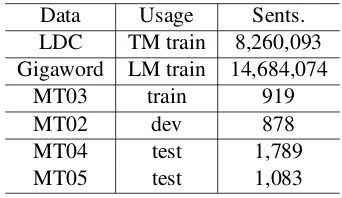
We conduct experiments on a large scale machine translation tasks. The parallel data comes from LDC, including LDC2002E18, LDC2003E14, LDC2004E12, LDC2004T08, LDC2005T10, LDC2007T09, which consists of 8.2 million of sentence pairs. Monolingual data includes Xinhua portion of Gigaword corpus. We use multi-references data MT03 as training data, MT02 as development data, and MT04, MT05 as test data. These data are mainly in the same genre, avoiding the extra consideration of domain adaptation.
Data Usage Sents.
LDC TM train 8,260,093
Gigaword LM train 14,684,074
MT03 train 919
MT02 dev 878
MT04 test 1,789
[image:6.595.324.495.587.686.2]MT05 test 1,083
Table 1: Experimental data and statistics.
The Chinese side of the corpora is word seg-mented using ICTCLAS3. Our translation
Criteria MT03(train) MT02(dev) MT04 MT05
BRc 35.02 36.63 34.96 34.15
BR 38.66 40.04 38.73 37.50
BW 39.55 39.36 38.72 37.81
[image:7.595.145.439.61.132.2]PW 38.61 38.85 38.73 37.98
Table 2: BLEU4 in percentage on different training criteria (”BR”, ”BW” and ”PW” refer to experiments with ”Best v.s. Rest”, ”Best v.s. Worst” and ”Pairwise” training criteria, respectively. ”BRc” indicates
generate hypothesis pairs from n-best set of current iteration only presented in Section 4.3.
tem is an in-house implementation of the hier-archical phrase-based translation system(Chiang, 2005). We set the beam size to 20. We train a 5-gram language model on the monolingual data with MKN smoothing(Chen and Goodman, 1998). For each parameter tuning experiments, we ran the same training procedure 3 times and present the average results. The translation quality is evalu-ated use 4-gram case-insensitive BLEU (Papineni et al., 2002). Significant test is performed using bootstrap re-sampling implemented by Clark et al. (2011). We employ a two-layer neural network with 11 input layer nodes, corresponding to fea-tures listed in Section 3.2 and 1 output layer node. The number of nodes in the hidden layer varies in different settings. The sigmoid function is used as the activation function for each node in the hidden layer. For the output layer we use a linear activa-tion funcactiva-tion. We try differentλfor the L1 norm
from 0.01 to 0.00001 and use the one with best performance on the development set. We solve the optimization problem with ALGLIB package4.
6.2 Experiments of Training Criteria
This set experiments evaluates different training criteria discussed in Section 4.1. We generate hypothesis-pair according to BW, BR and PW cri-teria, respectively, and perform training with these pairs. In the PW criterion, we use the sampling method of PRO (Hopkins and May, 2011) and get the 50 hypothesis pairs for each sentence. We use 20 hidden nodes for all three settings to make a fair comparison.
The results are presented in Table 2. The first two rows compare training with and with-out the weighted combination of hypothesis pairs we discussed in Section 4.3. As the result sug-gested, with the weighted combination of hypothe-sis pairs from previous iterations, the performance improves significantly on both test sets.
4http://www.alglib.net/
Although the system performance on the dev set varies, the performance on test sets are al-most comparable. This suggest that although the three training criteria are based on different as-sumptions, their are basically equivalent for train-ing translation systems.
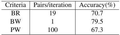
Criteria Pairs/iteration Accuracy(%)
BR 19 70.7
BW 1 79.5
[image:7.595.314.506.291.348.2]PW 100 67.3
Table 3: Comparison of different training criteria in number of new instances per iteration and train-ing accuracy.
We also compares the three training criteria in their number of new instances per iteration and final training accuracy (Table 3). Compared to BR which tries to separate the best hypothesis from the rest hypotheses in the n-best set, and PW which tries to obtain a correct ranking of all hy-potheses, BW only aims at separating the best and worst hypothesis of each iteration, which is a eas-ier task for learning a classifeas-iers. It requires the least training instances and achieves the best per-formance in training. Note that, the accuracy for each system in Table 3 are the accuracy each sys-tem achieves after training stops. They are not cal-culated on the same set of instances, thus not di-rectly comparable. We use the differences in accu-racy as an indicator for the difficulties of the cor-responding learning task.
For the rest of this paper, we use the BW crite-rion because it is much simpler compared to sam-pling method of PRO (Hopkins and May, 2011).
6.3 Experiments of Network Structures
Systems MT03(train) MT02(dev) MT04 MT05 Test Average
HPB 39.25 39.07 38.81 38.01 38.41
TLayer20 39.55∗ 39.36∗ 38.72 37.81 38.27(-0.14)
TLayer30 39.70+ 39.71∗ 38.89 37.90 38.40(-0.01)
TLayer50 39.26 38.97 38.72 38.79+ 38.76(+0.35)
TLayer100 39.42 38.77 38.65 38.65+ 38.69(+0.28)
TLayer200 39.69 38.68 38.72 38.80+ 38.74(+0.32)
TDN 39.60+ 38.94 38.99∗ 38.13 38.56(+0.15)
[image:8.595.103.486.60.186.2]GN 39.73+ 39.41+ 39.45+ 38.51+ 38.98(+0.57)
Table 4: BLEU4 in percentage for comparing of systems using different network structures (HPB refers to the baseline hierarchical phrase-based system. TLayer, TDN, GN refer to the standard 2-layer network, Two-Degree Hidden Layer Network, Grouped Network, respectively. Subscript of TLayer indicates the number of nodes in the hidden layer.) +, ∗ marks results that are significant better than the baseline
system withp <0.01andp <0.05.
Systems # Hidden Nodes # Parameters Training Time per iter.(s)
HPB - 11 1041
TLayer20 20 261 671
TLayer30 30 391 729
TLayer50 50 651 952
TLayer100 100 1,301 1,256
TLayer200 200 2,601 2,065
TDN 55 221 808
[image:8.595.135.466.271.394.2]GN 214 1,111 1,440
Table 5: Comparison of network scales and training time of different systems, including the number of nodes in the hidden layer, the number of parameters, the average training time per iteration (15 iterations). The notations of systems are the same as in Table4.
different systems5. All 5 two-layer feed forward
neural networks models could achieve compara-ble or better performance comparing to the base-line system. We can see that training a larger net-work may lead to better translation quality (from TLayer20 and TLayer30 to TLayer50). However,
increasing the number of hidden node to 100 and 200 does not bring further improvement. One pos-sible reason is that training a larger network with arbitrary connections brings in too many param-eters which may be difficult to train with limited training data.
TDN and GN are the two network structures proposed in Section 5. With the constraint that all input to the hidden node should be of degree 2, TDN performs comparable to the baseline sys-tem. With the grouped feature, we could design networks such as GN, which shows significant im-provement over the baseline systems (+0.57) and achieves the best performance among all neural systems.
5TLayer
20is the same system as BW in Table 2
Table 4 shows statistics related to the efficiency issue of different systems. The baseline system (HPB) uses MERT for training. HPB has a very small number of parameters and searches for the best parameters exhaustively in each iteration. The non-linear systems with few nodes (TLayer20and
TLayer30) train faster than HPB in each iteration
because they perform back-propagation instead of exhaustive search. We iterate 15 iterations for each non-linear system, while MERT takes about 10 rounds to reach its best performance.
When the number of nodes in the hidden layer increases (from 20 to 200), the number of param-eters in the system also increases, which requires longer time to compute the score for each hypoth-esis and to update the parameters through back-propagation. The network with 200 hidden nodes takes about twice the time to train for each itera-tion, compared to the linear system6.
TDN and GN have larger numbers of hidden
6Matrix operation is CPU intensive. The cost will
nodes. However, because of our intuitions in de-signing the structure of the networks, the degree of the hidden node is constrained. So these two networks are sparser in parameters and take sig-nificant less training time than standard neural net-works. For example, GN has a comparable num-ber of hidden nodes with TLayer200, but only has
half of its parameters and takes about 70% time to train in each iteration. In other words, our pro-posed network structure provides more efficient training in these cases and achieve better results.
7 Conclusion
In this paper, we discuss a non-linear framework for modeling translation hypothesis for statisti-cal machine translation system. We also present a learning framework including training criterion and algorithms to integrate our modeling into a state of the art hierarchical phrase based machine translation system. Compared to previous effort in bringing in non-linearity into machine transla-tion, our method uses a single two-layer neural networks and performs training independent with any previous linear training methods (e.g. MERT). Our method also trains its parameters without any pre-training or post-training procedure. Experi-ment shows that our method could improve the baseline system even with the same feature as input, in a large scale Chinese-English machine translation task.
In training neural networks with hidden nodes, we use heuristics to reduce the complexity of net-work structures and obtain extra advantages over standard networks. It shows that heuristics and in-tuitions of the data and features are still important to a machine translation system.
Neural networks are able to perform feature learning by using hidden nodes to model the in-teraction among a large vector of raw features, as in image and speech processing (Krizhevsky et al., 2012; Hinton et al., 2012). We are trying to model the interaction between hand-crafted fea-tures, which is indeed similar in spirit with learn-ing features from raw features. Although our fea-tures already have concrete meaning, e.g. the probability of translation, the fluency of target sen-tence, etc. Combining these features may have ex-tra advantage in modeling the ex-translation process. As future work, it is necessary to integrate more features into our learning framework. It is also in-teresting to see how the non-linear modeling fits
in to more complex learning tasks which involves domain specific learning techniques.
Acknowledgments
The authors would like to thank Yue Zhang and the anonymous reviewers for their valu-able comments. This work is supported by the National Natural Science Foundation of China (No. 61300158, 61223003), the Jiangsu Provin-cial Research Foundation for Basic Research (No. BK20130580).
References
Michael Auli and Jianfeng Gao. 2014. Decoder in-tegration and expected BLEU training for recurrent
neural network language models. In Proceedings
of the 52nd Annual Meeting of the Association for Computational Linguistics, ACL 2014, June 22-27, 2014, Baltimore, MD, USA, Volume 2: Short Papers, pages 136–142.
Michael Auli, Michel Galley, Chris Quirk, and Geof-frey Zweig. 2013. Joint language and translation
modeling with recurrent neural networks. In
Pro-ceedings of the 2013 Conference on Empirical Meth-ods in Natural Language Processing, EMNLP 2013, 18-21 October 2013, Grand Hyatt Seattle, Seattle, Washington, USA, A meeting of SIGDAT, a Special Interest Group of the ACL, pages 1044–1054.
Christopher M. Bishop. 1995. Neural Networks for
Pattern Recognition. Oxford University Press, Inc., New York, NY, USA.
Peter F. Brown, Stephen Della Pietra, Vincent J. Della Pietra, and Robert L. Mercer. 1993. The mathe-matic of statistical machine translation: Parameter
estimation. Computational Linguistics, 19(2):263–
311.
S. F. Chen and J. T. Goodman. 1998. An empirical study of smoothing techniques for language mod-eling. Technical report, Computer Science Group, Harvard University, Technical Report TR-10-98.
David Chiang. 2005. A hierarchical phrase-based
model for statistical machine translation. Inannual
meeting of the Association for Computational Lin-guistics.
David Chiang. 2012. Hope and fear for discriminative
training of statistical translation models. J. Mach.
Learn. Res., 13(1):1159–1187, April.
Jonathan H. Clark, Chris Dyer, Alon Lavie, and Noah A. Smith. 2011. Better hypothesis testing for statistical machine translation: Controlling for
Meeting of the Association for Computational Lin-guistics: Human Language Technologies: Short Pa-pers - Volume 2, HLT ’11, pages 176–181, Strouds-burg, PA, USA. Association for Computational Lin-guistics.
Jonathan Clark, Chris Dyer, and Alon Lavie. 2014. Locally non-linear learning for statistical machine translation via discretization and structured
regular-ization. Transactions of the Association for
Compu-tational Linguistics, 2:393–404.
Jacob Devlin, Rabih Zbib, Zhongqiang Huang, Thomas Lamar, Richard M. Schwartz, and John Makhoul. 2014. Fast and robust neural network joint models
for statistical machine translation. In Proceedings
of the 52nd Annual Meeting of the Association for Computational Linguistics, ACL 2014, June 22-27, 2014, Baltimore, MD, USA, Volume 1: Long Papers, pages 1370–1380.
Kevin Duh and Katrin Kirchhoff. 2008. Beyond log-linear models: Boosted minimum error rate
train-ing for n-best re-ranktrain-ing. In Proceedings of the
46th Annual Meeting of the Association for Compu-tational Linguistics on Human Language Technolo-gies: Short Papers, HLT-Short ’08, pages 37–40, Stroudsburg, PA, USA. Association for Computa-tional Linguistics.
Dumitru Erhan, Pierre antoine Manzagol, Yoshua Ben-gio, Samy BenBen-gio, and Pascal Vincent. 2009. The difficulty of training deep architectures and the
ef-fect of unsupervised pre-training. In David V.
Dyk and Max Welling, editors, Proceedings of the
Twelfth International Conference on Artificial In-telligence and Statistics (AISTATS-09), volume 5, pages 153–160. Journal of Machine Learning Re-search - Proceedings Track.
Jianfeng Gao, Xiaodong He, Wen-tau Yih, and Li Deng. 2014. Learning continuous phrase
repre-sentations for translation modeling. InProceedings
of the 52nd Annual Meeting of the Association for Computational Linguistics, ACL 2014, June 22-27, 2014, Baltimore, MD, USA, Volume 1: Long Papers, pages 699–709.
Geoffrey Hinton, Li Deng, Dong Yu, George E Dahl, Abdel-rahman Mohamed, Navdeep Jaitly, Andrew Senior, Vincent Vanhoucke, Patrick Nguyen, Tara N Sainath, et al. 2012. Deep neural networks for acoustic modeling in speech recognition: The shared
views of four research groups. Signal Processing
Magazine, IEEE, 29(6):82–97.
Mark Hopkins and Jonathan May. 2011. Tuning as
ranking. In Proceedings of the Conference on
Em-pirical Methods in Natural Language Processing, EMNLP ’11, pages 1352–1362, Stroudsburg, PA, USA. Association for Computational Linguistics. Liang Huang and David Chiang. 2007. Forest
rescor-ing: Faster decoding with integrated language
mod-els. InProceedings of the 45th Annual Meeting of
the Association of Computational Linguistics, pages 144–151, Prague, Czech Republic, June. Associa-tion for ComputaAssocia-tional Linguistics.
Philipp Koehn, Franz Josef Och, and Daniel Marcu.
2003. Statistical phrase-based translation. In
HLT-NAACL.
Alex Krizhevsky, Ilya Sutskever, and Geoffrey E. Hin-ton. 2012. Imagenet classification with deep con-volutional neural networks. In F. Pereira, C.J.C. Burges, L. Bottou, and K.Q. Weinberger, editors,
Advances in Neural Information Processing Systems
25, pages 1097–1105. Curran Associates, Inc.
Quoc V. Le, Jiquan Ngiam, Adam Coates, Ahbik Lahiri, Bobby Prochnow, and Andrew Y. Ng. 2011.
On optimization methods for deep learning. In
Pro-ceedings of the 28th International Conference on Machine Learning, ICML 2011, Bellevue, Washing-ton, USA, June 28 - July 2, 2011, pages 265–272. Yang Liu, Qun Liu, and Shouxun Lin. 2006.
Tree-to-string alignment template for statistical machine
translation. InProceedings of the 44th Annual
Meet-ing of the Association of Computational LMeet-inguistics. The Association for Computer Linguistics.
Lemao Liu, Taro Watanabe, Eiichiro Sumita, and Tiejun Zhao. 2013. Additive neural networks for
statistical machine translation. In Proceedings of
the 51st Annual Meeting of the Association for Com-putational Linguistics, ACL 2013, 4-9 August 2013, Sofia, Bulgaria, Volume 1: Long Papers, pages 791– 801.
Shixiang Lu, Zhenbiao Chen, and Bo Xu. 2014. Learning new semi-supervised deep auto-encoder
features for statistical machine translation. In
Pro-ceedings of the 52nd Annual Meeting of the Asso-ciation for Computational Linguistics (Volume 1: Long Papers), pages 122–132, Baltimore, Maryland, June. Association for Computational Linguistics. Sameer Maskey and Bowen Zhou. 2012.
Unsuper-vised deep belief features for speech translation. In
INTERSPEECH 2012, 13th Annual Conference of the International Speech Communication Associa-tion, Portland, Oregon, USA, September 9-13, 2012. Franz Josef Och and Hermann Ney. 2002. Discrimina-tive training and maximum entropy models for sta-tistical machine translation. pages 295–302. Franz Josef Och. 2003. Minimum error rate
train-ing in statistical machine translation. InACL ’03:
Proceedings of the 41st Annual Meeting on Asso-ciation for Computational Linguistics, pages 160– 167, Morristown, NJ, USA. Association for Compu-tational Linguistics.
Kishore Papineni, Salim Roukos, Todd Ward, and Wei-Jing Zhu. 2002. Bleu: a method for automatic
eval-uation of machine translation. InACL ’02:
Computational Linguistics, pages 311–318, Morris-town, NJ, USA. Association for Computational Lin-guistics.
Robert E. Schapire. 1999. A brief introduction to
boosting. InProceedings of the 16th International
Joint Conference on Artificial Intelligence - Volume
2, IJCAI’99, pages 1401–1406, San Francisco, CA,
USA. Morgan Kaufmann Publishers Inc.
Ashish Vaswani, Yinggong Zhao, Victoria Fossum, and David Chiang. 2013. Decoding with large-scale neural language models improves translation. In
Proceedings of the 2013 Conference on Empirical Methods in Natural Language Processing, EMNLP 2013, 18-21 October 2013, Grand Hyatt Seattle, Seattle, Washington, USA, A meeting of SIGDAT, a Special Interest Group of the ACL, pages 1387– 1392.
Taro Watanabe. 2012. Optimized online rank learning
for machine translation. InProceedings of the 2012
Conference of the North American Chapter of the Association for Computational Linguistics: Human Language Technologies, NAACL HLT ’12, pages 253–262, Stroudsburg, PA, USA. Association for Computational Linguistics.
Kenji Yamada and Kevin Knight. 2001. A
syntax-based statistical translation model. InProceedings