Implicit Feature Selection with the Value Difference Metric

letter

c

1998 T.R.Payne and P.Edwards

ECAI 98.13th European Conference on Artificial Intelligence Edited by Henri Prade

Implicit Feature Selection with the Value

Difference Metric

Terry R. Payne

and

_{Peter Edwards}

Abstract. The nearest neighbour paradigm provides an

effective approach to supervised learning. However, it is es-pecially susceptible to the presence of irrelevant attributes. Whilst many approaches have been proposed that select only the most relevant attributes within a data set, these ap-proaches involve pre-processing the data in some way, and can often be computationally complex. The Value Difference Metric (VDM) is a symbolic distance metric used by a number of different nearest neighbour learning algorithms. This paper demonstrates how the VDM can be used to reduce the impact of irrelevant attributes on classification accuracy without the need for pre-processing the data. We illustrate how this metric uses simple probabilistic techniques to weight features in the instance space, and then apply this weighting technique to an alternative symbolic distance metric. The resulting distance metrics are compared in terms of classification accuracy, on a number of real-world and artificial data sets.

1

INTRODUCTION

The task of a supervised learning algorithm is to utilise pre-classified training instances to induce a classification hypoth-esis that can subsequently be used to classify new instances. These instances are normally presented as fixed length fea-ture vectors, where each element in the vector corresponds to some property or attribute of the data. The task of deter-mining which of these attributes are relevant to the classifica-tion task is one of the central problems in machine learning. Ideally, the learning algorithm would be presented with only relevant attributes, and thus any problems associated with ir-relevant attributes would be eliminated. However, as data sets become more complex, the number of irrelevant attributes in-herent in the data increases, and thus can have a detrimental effect on the accuracy of the classification algorithm. Thus, it is important to identify such attributes automatically and prevent them from influencing the classification process.

One of the most common learning paradigms in machine learning and pattern analysis is the Nearest Neighbour (NN) paradigm. This approach to supervised learning has been studied extensively [6], and compared with a variety of other learning approaches, such as Bayesian techniques [14], artifi-cial neural networks [12] and rule induction algorithms [12], and has also been analysed theoretically [10]. Variants on the nearest neighbour theme have also been proposed that repre-sent the induced hypothesis as hyper-rectangles [15], as a set of prototype points or selected instances [2, 4], or as feature projections [3].

1

Department of Computing Science, King’s College, University of Aberdeen, Aberdeen, Scotland, AB24 3UE.

2

Department of Computing Science, King’s College, University of Aberdeen, Aberdeen, Scotland, AB24 3UE.

Nearest Neighbour learning algorithms determine the class label of an unclassified instance by comparing it to a set of stored, classified instances, and identifying the class label of the nearest neighbour in this set. As the distance between the unclassified instance and each stored instance is determined from the values of each attribute, this approach is suscepti-ble to the presence of irrelevant attributes. As a result, the accuracy of NN algorithms will generally degrade if irrelevant attributes exist within the data set.

This paper investigates the irrelevant attribute problem, and briefly examines a number of existing approaches used to overcome it. The role of the distance metric is studied and we show how one specific symbolic distance metric, the Value Difference Metric (VDM) overcomes the irrelevant attribute problem without the need for additional processing.

In the next section, a brief introduction to Nearest Neigh-bour learning is presented, and the VDM is described. In the third section, a variety of attribute selection approaches are presented. We show how the VDM can reduce the effect of irrelevance in the fourth section, and evaluate this property empirically. The paper concludes in the final section.

2

NEAREST NEIGHBOUR LEARNING

AND THE VALUE DIFFERENCE

METRIC

The nearest neighbour (or instance-based) learning paradigm is based on the assumption that instances in close proximity to each other within an instance space will have similar posterior class probabilities. In other words, if two instances are very similar, i.e. they are close to each other within the instance space, then they will share the same class label. Hence, if the class of a new instance is unknown, it can be predicted by determining the class of its nearest neighbour within this instance space.

To determine the proximity of two instances, a distance metric is required. Although several distance metrics have been proposed [19], the most commonly used metrics are suit-able only for either symbolicornumeric attributes. These in-clude theEuclidean andManhattan distance metrics for nu-meric attributes, and theOverlapdistance metric for symbolic attributes. These metrics calculate the distance between two instances by determining the difference between the values for each attribute (2), and combining these differences to gener-ate an overall distance value (1)3

:

3

The value ofr_{in (1) varies for theMinkowskianmetric, but is}

equal to 1 for theOverlapmetric. c

1998 T.R.Payne P.Edwards

D(i, j) =

"A

X

a=0

δ(ia, ja)

#1r

(1)

δ(ia, ja) = 8 <

:

0 ifia=ja(Overlap) 1 ifia6=ja(Overlap)

|ia−ja|r (Minkowskian)

(2)

Here,iandjrefer to the two instances, andarefers to one of theAattributes. The distance metrics described above dif-fer in the approach used to compare the two valuesiaandja in (2). TheOverlapmetric simply compares the two symbolic values; if they are the same then it returns a value of zero, oth-erwise a value of one is returned. TheEuclideanand Manhat-tandistance metrics are both special cases of theMinkowskian distance metric, and differ in the value used forr, wherer= 2 for theEuclideandistance metric, andr= 1 for the Manhat-tandistance metric4

.

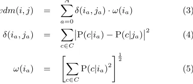
TheValue Difference Metric(VDM) was first proposed as an alternative approach for determination of the distance be-tween two symbolic values [17]. It differs from other distance metrics in that the distance between two attribute values is determined by comparing the class conditional probability distributions for the valuesiaandjafor each attributea(4).

vdm(i, j) = A X

a=0

δ(ia, ja)·ω(ia) (3)

δ(ia, ja) = X

c∈C ˛

˛P(c|ia)−P(c|ja)

˛ ˛ 2

(4)

ω(ia) = "

X

c∈C P(c|ia)

2

#1

2

(5)

Here, C is the set of all class labels present in the data set, and P(c|ia) is the class conditional probability ofia, i.e. the probability of the valueia occurring in the data set for attributea in instances of classc. This probability is deter-mined directly from the training data by counting the number of instances containing the valueia for attributea, and de-termining the proportion that also have the class labelc, i.e.:

P(c|ia) =

|instances containingia∧class =c|

|instances containingia|

ia= ‘X’ ia= ‘Y’ ia= ‘Z’ P(c1|ia) 0.7 0.4 0.6

P(c_2|i_{a) 0.0 0.5 0.1}

P(c3|ia) 0.3 0.1 0.3

Table 1. Class Conditional Probability Values for the symbols in Figure 1.

This process can be illustrated by means of an example. The top three charts in Figure 1 represent the discrete class distributions of three different symbolic values, ‘X’, ‘Y’ and 4

A comparison of these two metrics can be found in [16]

c₁ c₂ c3 c1 c2 c3

c1 c2 c3 c1 c2 c3

c1 c2 c3

Comparing ‘X’ with ‘Y’ Comparing ‘X’ with ‘Z’ Symbolic Value ‘Z’ Symbolic Value ‘Y’

Symbolic Value ‘X’

Class Class

Class Class Class

Probability

Probability

Probability

Probability

Probability

Figure 1. Comparing symbolic values with the Value Difference Metric.

‘Z’. Each distribution consists of three class conditional prob-abilities, represented by the vertical bars. The lower charts illustrate how pairs of symbolic values are compared. For each class, the difference (4) in class conditional probability is de-termined (i.e. the difference in height between the vertical bars). These differences are then combined (3) and result in a distance measure for the two symbolic values of attribute

a. Hence, to compute the distance between the two symbols ‘X’ and ‘Y’, the difference in class conditional probabilities is found for each class. For this example, the differences are 0.3, -0.5 and 0.2 for classes c1, c2 and c3 respectively (the class conditional values for these symbols are listed in Table 1). Hence the final distance between the two symbols is the sum of the squares of these distances = 0.38, i.e.

δ(‘X’,‘Y’) = 0.32

+ (−0.5)2 + 0.22

= 0.38

The weight component of the VDM (5) provides some in-dication of how well an attribute value discriminates between different class labels. The weight can vary between a mini-mum which is dependent on the number of classes present in the data set, and 1 which represents an ideal discriminator, i.e. an attribute value which only appears in one class. The minimum represents a uniform class distribution where an at-tribute value appears with equal probability in instances of all classes, and can be calculated as follows (6):

ω(u) =|C|−0.5

(6) where ω(u) is this minimum value (i.e. the weight of an attribute value with a uniform class distribution), and C is the set of all class labels that appear in the data set.

The weight is used to control the influence of the attribute distance for each training instance when determining the fi-nal nearest neighbour. As the range of values ofδ(ia, ja) will vary between zero and one, the weight can be used to restrict this range, i.e. the range ofδ(ia, ja)·ω(ia) will vary between zero andω(ia). A large attribute distance will have a greater

effect on the value of vdm(i, j) than a smaller one. Thus if a small weight is used (i.e. the value present in the test in-stance is irrelevant), then the resulting attribute diin-stance will also be small and have little impact on the choice of nearest neighbour.

Many Nearest Neighbour learning algorithms employ weights to modify the effect a specific component has in the resulting classification process [1, 8, 15, 18]. For example, PE-BLS [5] and EACH [15] assign a weight to each of the instances (or hyper-rectangles in the case of EACH) and modify this weight according to whether the instances result in correct or incorrect class predictions. The weight is used to measure the reliability of an instance, and hence reduce the detrimental effects of noisy instances. The VDM utilises value weights (5) to determine how well a specific value for a given attribute can discriminate between class labels. Other systems utilise weights to augment (or diminish) the effects of relevant (or irrelevant) attributes [1, 15].

3

IRRELEVANT ATTRIBUTES AND

FEATURE SELECTION

An attribute is irrelevant if it contributes nothing to the target hypothesis, i.e. it makes no meaningful contribution towards the classification task. At best, such attributes increase the dimensionality of the data set, and thus increase the space required to store the data set, and the computational cost of inducing a hypothesis. However, the inclusion of such at-tributes often also results in a degradation in classification accuracy.

Nearest Neighbour algorithms are especially susceptible to the inclusion of irrelevant attributes in the data set, and sev-eral studies have shown that the classification accuracy de-grades as the number of irrelevant attributes is increased [1, 10, 18]. This degradation is due to the fact that irrele-vant attributes violate the underlying assumption made by the nearest neighbour paradigm. As the location of the in-stance is defined by its attributes, this assumption relies on the attributes being relevant to the target hypothesis.

Attribute selection is the process of identifying a small sub-set of relevant attributes from the attributes present in the data set. The resulting data set will generally contain fewer irrelevant attributes, and thus the performance of the learn-ing algorithm will increase in terms of either complexity of the target hypothesis, or in terms of accuracy. A number of different techniques have been studied [13], and can be grouped into two broad categories: those that employ the fil-termodel, where the selection technique is independent of the final learning algorithm; and those that employ thewrapper model, where the final learning algorithm is embedded within the selection mechanism. The wrapper model was proposed as a means of using the bias inherent in the learning algo-rithm, to select the attribute subset. It has been argued that this model is superior to the filter model, which uses differ-ent biases in the attribute selection and the learning stages [7]. Both models perform a search within a space of attribute subsets to determine the optimal (or sub-optimal) subset for the classification task.

In contrast to these models, a number of nearest neighbour techniques utilise weights to identify irrelevant attributes. At-tribute weights are determined by evaluating the NN

algo-rithm on the training data. A vector of attribute weights is generated, which initially gives each attribute an equal weight. The leave-one out cross validation technique [9] is then used to predict the class label of each of the instances in the data set. As each instance is evaluated, the weights are adjusted according to whether or not the classification is correct. An example of a weight update function is given in (7), whereωa is the weight of the attributea;iaandjaare the values of the attributeain instancesiandj; andµis an incremental value (such as 0.02) which is positive when a correct classification is predicted, and negative when an incorrect classification is made.

ωa = 

ωa(1 +µ) ifia=ja

ωa(1−µ) ifia6=ja (7) The intuition behind this model is that irrelevant attributes will contribute very little overall to the classification task. The function used to update the weights is designed to reward those attributes if they are responsible for making correct predictions, and penalise them if they are responsible for in-correct ones. Thus, the contribution of irrelevant attributes to the classification task falls as the contribution of other at-tributes rises. The resulting weights can be used to determine which attributes should be retained in the attribute subset, and which attributes should be discarded [8]. An alternative approach is to use the weights to control the influence that each attribute has on the distance between two instances. Those attributes which are awarded low weights will have a diminished effect on the resulting class predictions.

4

EVALUATION OF THE VDM FOR

IMPLICIT FEATURE SELECTION

The Value Difference Metric differs from many other distance metrics in that the location of an instance within the instance space is not defined directly by the values of its attributes, but by the class conditional distributions of these values. The dis-tributions vary from being skewed, where an attribute value appears in instances of only one class, to a uniform distribu-tion, where the attribute value appears equally in instances of each class. In other words, attribute values with skewed distributions may be highly relevant to the target concept, and attribute values with a uniform distribution may be ir-relevant. However, these distributions assume that each at-tribute value is independent of any other value for any of the attributes. The value weight componentω(ia) provides some indication of the skew of the class distribution for an attribute value, and can be used to control the influence each attribute distance has on the final distancevdm(i, j).

We have investigated the utility of ω(ia), both as a com-ponent of the VDM, and when combined with another dis-tance metric. Several symbolic data sets from the UCI Ma-chine Learning Repository [11] were used to evaluate the per-formance of five distance metrics: three of which were based on class conditional probabilities (VDM, MVDM & OMVW); and two which were used for baseline comparisons with other studies. The MVDM differs from the metric given in (3) in that the term ω(ia) is omitted. In contrast, the OMVW utilises the value weight (5), but instead of using the attribute distance defined in (4), the attribute distance for the Overlap metric (2) is used.

The weighted Overlap metric (WOM) and the simple Over-lap metric (OM) were included to provide a comparison of the VDM, MVDM and OMVW with other distance metrics. The Weighted Overlap metric (WOM) is similar to the distance metrics used by weighted NN algorithms, such as IB4 [1] and EACH [15]. A set of attribute weights are generated by eval-uating the training data and updating the attribute weights

ωa using the weight function given in (7). The WOM and OMVW differ in that the weights used by the OMVW are probabilistic and can be rapidly determined from the train-ing set, whereas the weights in the WOM are induced, and thus require a separate training stage.

Three hypotheses were investigated:

H1 There is no difference between the performance of MVDM and VDM, i.e.ω(ia) has no significant effect on the perfor-mance of the VDM.

H2 The value weight componentω(ia) of the VDM can be effectively utilised by the Overlap metric to improve per-formance in terms of accuracy. The perper-formance of the OMVW should be comparable to that of the WOM, and both metrics should achieve better results (in general) than the OM.

H3 The use of class conditional probabilities within the dis-tance metric should improve the classification accuracy by reducing the effects of irrelevant attributes, i.e. the per-formance of the VDM, MVDM and OMVW should not degrade in the presence of irrelevant attributes.

OM WO M

OM VW

MV DM

VD M

Breast-cancer 70.73 66.44 71.46 67.51 67.16 Lung-cancer 40.00 40.00 46.67 68.33 65.00 Lymphography 81.24 82.57 83.24 83.24 83.19 Primary-tumor 32.05 32.07 33.54 30.83 31.15 Promoters 77.00 82.73 79.73 89.36 87.36 Tic-tac-toe 80.90 82.88 72.75 90.71 90.71 Votes 92.44 94.73 93.80 94.51 94.97

Zoo 96.09 95.09 95.09 97.09 97.09

Table 2. 10-fold cross validated classification accuracies.

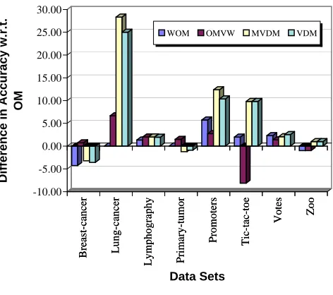
To evaluate the performance of each of the distance metrics, a 10-fold cross validation [9] was performed on a number of different UCI data sets. The results, given in Table 2, list the classification accuracies achieved by each metric for each of the data sets. Results presented in bold were found to be sig-nificantly higher (p=0.05) than those achieved by the Overlap

metric (OM), whereas those in italics were significantly lower. A one-tailed paired t-test was used to determine this signifi-cance. Figure 2 plots the difference in the results obtained by the OM and the other distance metrics.

Breast-cancer Lung-cancer

Lymphography Primary-tumor

Promoters _Tic-tac-toe

Votes Zoo

-10.00 -5.00 0.00 5.00 10.00 15.00 20.00 25.00 30.00

Difference in Accuracy w.r.t.

OM

Breast-cancer Lung-cancer

Lymphography Primary-tumor

Promoters _Tic-tac-toe

Votes Zoo

Data Sets

WOM OMVW MVDM VDM

Figure 2. Comparison of the 10 fold cross validated classification accuracies of the distance metrics relative to the

Overlap metric (OM).

There was no significant difference between the perfor-mance of the VDM and MVDM for any of the data sets, which appears to support H1. The VDM succeeded in signifi-cantly improving the classification accuracy for four data sets (p=0.05), and succeeded in raising the accuracy (though not significantly) for two other data sets. The MVDM achieved similar success, except for theVotesdata set, where the in-crease in accuracy became significant whenp=0.054. The re-sults for both distance metrics were significantly lower than the OM for only one data set (Breast-Cancer). These results demonstrate that the VDM (and MVDM) can achieve better classification accuracies than the Overlap metric. The accu-racy of the MVDM was significantly higher than the WOM for three data sets (Lung-cancer,PromotersandTic-tac-toe). The OMVW also succeeded in raising the classification ac-curacy for six of the data sets, although the increase was only significant for three. A significant increase in accuracy was also achieved by the WOM for two of the same three data sets. As the WOM has previously been demonstrated to be robust in the presence of irrelevant attributes, and given that a similar increase in accuracy can be observed for the OMVW, this suggests that the value weightω(ia) can be used to limit the impact of irrelevant attributes on the classification accu-racy. This appears to support H2.

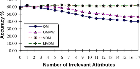
Although the distance metrics based on the VDM per-formed well with the data sets, a further investigation was required to determine if the performance of these metrics would degrade in the presence of irrelevant attributes. For this reason, the metrics were evaluated on the 24-attribute LED display problem. This problem contains seven binary valued attributes (corresponding to the different segments

within an LED seven segment numeric display), and an ad-ditional seventeen irrelevant attributes [2]. If this number of additional attributes is varied, it is possible to observe the effect of irrelevant attributes on different learning algorithms. Data sets were constructed containing 200 randomly gener-ated instances with 10% noise (i.e. each attribute value had a 10% chance of being inverted). The number of irrelevant attributes was varied from zero to seventeen, and each test was repeated ten times. The results are plotted in Figure 3.

0.00 10.00 20.00 30.00 40.00 50.00 60.00 70.00

0 1 2 3 4 5 6 7 8 9 10 11 12 13 14 15 16 17

Number of Irrelevant Attributes

Accuracy %

OM

OMVW

VDM

MVDM

Figure 3. LED artificial results.

As the number of irrelevant attributes increased, the perfor-mance of the Overlap metric (OM) fell from 59.7% to 40.0%. There was a similar degradation in the performance of the OMVW, although this degradation was not as acute as the OM, and the classification accuracy of the OMVW was signif-icantly higher than that of the OM when three or more irrel-evant attributes were present. The VDM and MVDM showed no signs of degradation as the number of irrelevant attributes increased. These results support both H2 and H3, though it would appear thatω(ia) succeeds only in reducing the impact of the irrelevant attributes, not eliminating their effects.

5

CONCLUSIONS

The Value Difference Metric is an alternative symbolic dis-tance metric which can be successfully applied to classifica-tion problems containing irrelevant attributes. The distance metric utilises a set of value weights, which can be determined ‘on the fly’ from the training data. These value weights modify the distance between attribute values such that the distances between class discriminant values are augmented, but other-wise diminished. The exclusion of these value weights appears to have no effect on the performance of the VDM. However, if combined with the Overlap metric, the value weights im-prove the performance of the distance metric (in terms of accuracy) on data containing irrelevant attributes. This in-crease in performance is comparable to that achieved when attribute weights are induced, and utilised by the Overlap metric. However, the value weights have the advantage that no training is required.

ACKNOWLEDGEMENTS

T.R. Payne acknowledges financial support provided by the UK Engineering & Physical Sciences Research Council (EP-SRC).

REFERENCES

[1] D.W. Aha, ‘Tolerating Noisy, Irrelevant and Novel Attributes in Instance-Based Learning Algorithms’,International Jour-nal of Man-Machine Studies,36, 267–287, (1992).

[2] D.W. Aha, D. Kibler, and M.K. Albert, ‘Instance-Based Learning Algorithms’,Machine Learning,6, 37–66, (1991). [3] A. Akku¸s and H.A. G¨uvenir, ‘K Nearest Neighbor

Classifica-tion on Feature ProjecClassifica-tions’, in Proceedings of the 13th In-ternational Conference on Machine Learning, pp. 12–19. San Francisco, CA:Morgan Kaufmann, (1996).

[4] Y. Biberman, ‘The Role of Prototypicality in Exemplar-Based Learning’, in Proceedings of the 8th European Conference on Machine Learning, pp. 77–91. Berlin, Germany:Springer-Verlag, (1995).

[5] S. Cost and S. Salzberg, ‘A Weighted Nearest Neighbor Algo-rithm for Learning with Symbolic Features’,Machine Learn-ing,10, 57–78, (1993).

[6] B. V. Dasarathy,Nearest Neighbor(NN) Norms: NN Pattern Classification Techniques, Los Alamitos, California:IEEE Computer Society Press, 1991.

[7] G. John, R. Kohavi, and K. Pfleger, ‘Irrelevant Features and the Subset Selection Problem’, inProceedings of the 11th In-ternational Conference on Machine Learning, pp. 121–129. San Francisco, CA:Morgan Kaufmann, (1994).

[8] K. Kira and L.A. Rendell, ‘The Feature Selection Problem: Traditional Methods and a New Algorithm’, in Proceedings of the 10th National Conference on Artificial Intelligence (AAAI-92), pp. 129–134. MIT Press, (1992).

[9] R. Kohavi, ‘A Study of Cross-Validation and Bootstrap for Accuracy Estimation and Model Selection’, inProceedings of the 14th International Joint Conference on Artificial Intelli-gence (IJCAI), pp. 1137–1145. San Mateo, CA:Morgan Kauf-mann, (1995).

[10] P. Langley and W. Iba, ‘Average-case Analysis of a Nearest Neighbor Algorithm’, inProceedings of the 13th International Joint Conference on Artificial Intelligence (IJCAI), pp. 889– 894. San Mateo, CA:Morgan Kaufmann, (1993).

[11] C.J. Merz and P.M. Murphy. UCI repository of machine learn-ing databases, 1996.

[12] Machine Learning, Neural and Statistical Classification, eds., D. Michie, D.J. Spiegelhalter, and C.C. Taylor, UK:Ellis Hor-wood Ltd., 1994.

[13] T.R. Payne and P. Edwards, ‘A Survey of Feature Selection Methods’. Unpublished Draft, 1998.

[14] J. Rachlin, S. Kasif, S. Salzberg, and D.W. Aha, ‘Towards a Better Understanding of Memory-Based Reasoning Systems’, in Proceedings of the 11th International Machine Learning Conference (ML94), pp. 242–250. San Francisco, CA:Morgan Kaufmann, (1994).

[15] S. Salzberg, ‘A Nearest Hyperrectangle Learning Method’, Machine Learning,6, 251–276, (1991).

[16] S. Salzberg, ‘Distance Metrics for Instance-Based Learning’, inISMIS’91 6th International Symposium, Methodologies for Intelligent Systems, pp. 399–408, (1991).

[17] C. Stanfill and D. Waltz, ‘Toward Memory-Based Reasoning’, Communications of the ACM,29(12), 1213–1228, (1986). [18] D. Wettschereck, D.W. Aha, and T. Mohri, ‘A Review and

Empirical Evaluation of Feature Weighting Methods for a Class of Lazy Learning Algorithms’,Artificial Intelligence Re-view,11(1-5), 273–314, (1997). Special Issue on Lazy Learn-ing.