An Adaptive Multi-population Artificial Bee Colony Algorithm for Dynamic Optimisation Problems
Shams K. Nseef1, Salwani Abdullah1, Ayad Turky2 and Graham Kendall3,4
1Data Mining and Optimisation Research Group, Centre for Artificial Intelligence Technology,
Universiti Kebangsaan Malaysia, 43600 Bangi, Selangor, Malaysia. E-mail: [email protected]; [email protected]
2Swinburne University of Technology, Melbourne, Victoria, Australia
E-mail: [email protected]
3University of Nottingham Malaysia Campus, Semenyih, Malaysia
4ASAP Research Group, University of Nottingham, Nottingham, United Kingdom
Email: [email protected]; [email protected]
Abstract
Recently, interest in solving real-world problems that change over the time, so called dynamic optimisation problems (DOPs), has grown due to their practical applications. A DOP requires an optimisation algorithm that can dynamically adapt to changes and several methodologies have been integrated with population-based algorithms to address these problems. Multi-population algorithms have been widely used, but it is hard to determine the number of populations to be used for a given problem. This paper proposes an adaptive multi-population artificial bee colony (ABC) algorithm for DOPs. ABC is a simple, yet efficient, nature inspired algorithm for addressing numerical optimisation, which has been successfully used for tackling other optimisation problems. The proposed ABC algorithm has the following features. Firstly it uses multi-populations to cope with dynamic changes, and a clearing scheme to maintain the diversity and enhance the exploration process. Secondly, the number of sub-populations changes over time, to adapt to changes in the search space. The moving peaks benchmark DOP is used to verify the performance of the proposed ABC. Experimental results show that the proposed ABC is superior to the ABC on all tested instances. Compared to state of the art methodologies, our proposed ABC algorithm produces very good results.
Keywords: dynamic optimisation, artificial bee colony algorithm, adaptive multi-population method, meta-heuristics
1. Introduction
Many real-world optimisation problems have the characteristic of changing over time in terms of decision variables, constraints and the objective function [1], [2]. These problems *Revised Manuscript (changes marked)
are referred to as dynamic optimisation problems (DOPs) in the scientific literature. A DOP requires an optimisation algorithm that can dynamically adapt to the changes and track the optimum solution during the execution of the algorithm [2]. Given their practical applications and complexity, DOPs have attracted a lot of research attention. Population-based algorithms, which are a set of methodologies that utilise a population of solutions distributed over the search space, have attracted particular attention, due to their good performance [1], [2]. A key challenge in developing an optimisation algorithm for DOPs is how to maintain population diversity during the search process in order to keep track of landscape changes [3]. Several interesting diversity schemes have been developed in order to improve the search capability of population-based algorithms so that they can adapt effectively to the problem as it changes.
training process does not capture real world scenarios and there is a possibility of training errors due to lack of training data [7], [2].
Memory based methodologies aim to maintain diversity. They use a memory with a fixed size to store some of promising solutions that are captured during the search process. When a change is detected, the stored solutions will be reinserted into the current population and the population will be filtered to include only the best solutions. Examples of memory based methodologies can be found in [8], [9], [10], [11]. These methodologies have worked well when the dynamic problems are periodical or cyclic. The drawback is that they have parameter sensitivities that need to be determined in advance, and most real world problems are not cyclic in nature.
very good results when tested on the MPB. Turky and Abdullah [19] proposed a multi-population electromagnetic algorithm for DOPs. The proposed algorithm divides the population into several sub-populations to simultaneously explore and exploit the search process. The algorithm was tested on MPB problems and obtained very good results when compared to other population diversity mechanisms. The same authors [20] also presented a multi-population harmony search algorithm for the DOP. The population is divided into sub-populations. Each sub-population is responsible for either exploring or exploiting the search space. An external archive is utilised to track the best solutions found so far, which are used to replace the worst ones when a change is detected. The results show that this algorithm produces good results when compared to other methods. Sharifi et al. [21] proposed a hybrid PSO and local search algorithm for DOPs. The algorithm utilises a fuzzy social-only model to locate the peaks. The results show that this algorithm can produce very good results for MPB problems. In Li et al. [22] comprehensive experimental analysis was reported on the performance of a multi-population method with various algorithms in relation to DOPs. The authors concluded that the multi-population method is able to deal effectively with various DOPs and has the ability to maintain population diversity. It is also able to help the search in locating a new area through a divide and merge process and information exchange. The authors also highlighted several weaknesses of their method that relate to the number of sub-populations, the distribution of solutions and the reaction to problem changes.
Existing works on DOPs demonstrate that employing multi-population methods are the most effective method in maintaining population diversity. The features that make the multi-population methodologies popular are [3]: i) it divides the multi-population into sub-multi-populations, where the overall population diversity can be maintained since different populations can be located in different areas of the problem landscape, ii) it has the ability to search different areas simultaneously, enabling it to track the movement of the optimum, and iii) various single population-based algorithms can be integrated within multi-population methods.
divide the population into sub-populations, rather than focussing on diversification. To address these issues, this work proposes an adaptive multi-population artificial bee colony (ABC) algorithm for the DOP. The proposed ABC utilises a clearing scheme to remove redundant solutions in order to maintain diversity and enhance the exploration process. To efficiently track the landscape changes, the proposed ABC algorithm adaptively updates the number of sub-populations based on the problem change strength.
In this paper, the key objectives are:
i. To propose an artificial bee colony algorithm that utilises a multi-population and a population clearing scheme to efficiently solve the dynamic optimisation problem. ii. To propose an adaptive multi-population algorithm that updates the number of the
sub-populations based on the problem change strength.
iii. To test the performance of the proposed algorithm on dynamic optimisation problems using different scenarios and compare the results with other methodologies.
We used the moving peaks benchmark DOP with a different number of peaks to evaluate the effectiveness of the proposed ABC. Results demonstrate that the proposed ABC performs better than a basic ABC on all tested scenarios. Compared to the state of the art method, the proposed ABC produces very good results for many instances.
2. The proposed algorithm
This section presents the basic artificial bee colony algorithm, as well as our proposed adaptive multi-population algorithm.
2.1 Basic artificial bee colony algorithm
quality (objective function) of the problem being addressed. The three types of bees work together in an iterative manner to improve the quality of the population of solutions (food sources). The pseudo-code of a basic ABC is shown in Algorithm 1 [24]. ABC first sets the main parameters, initializes the population of solutions and then evaluates them. Next, the main loop is executed in an attempt to solve the given optimisation problem by calling the employee bees, onlooker bees and scout bees until the stopping condition is satisfied.
Algorithm 1: The pseudo-code of basic ABC
Step 1: Set the parameter values
Step 2: Initialize the population of solutions
Step 3: Evaluate the population of solutions
while termination condition is not met do Step 4: Employed Bees step
Step 5: Onlooker Bees step
Step 6: Scout Bees step
end while
The basic ABC has the following steps:
Step 1- Set ABC parameters. In this step the main parameters of ABC are initialized.
These include: the maximum number of iterations (MaxIt) which represents the stopping condition of ABC, the number of solutions or population size (Ps) which represent how many solutions will be generated, the total number of bees (Sbees) which is set to be twice the size of Ps, where half of them are employee bees and the other half are onlooker bees, the limit parameter (Lit), which is used to determine if the solution should be replaced by a new one.
Step 2- Initialise the population of solutions. A set of solutions with size equal to Ps are randomly generated as follows:
) ](
1 , 0
[ min
, max
, min
,
,j ij i j i j
i x Rand x x
x (1)
where i is the index of the solution, j is the current decision variable, Rand [0,1] generates a random number between zero and one and min
,j i
x and ximax,j are the lower and
Step 3- Evaluate the population of solutions. The fitness (quality) of the generated solutions are calculated using the objective function. The objective function is problem dependent. The objective function used in this work is shown in Section 3.2.
Step 4- Employed bees. Each employee bee is sent to one food source (solution). Its main role is to explore the neighbourhood of the current solution, seeking an improving solution. A neighbourhood solution, v, is created by modifying the ith solution, x, as follows:
)
( , ,
, ,
,j ij ij i j k j
i x x x
v (2)
where k is a randomly selected solution from Ps and Φ is a random number between [-1, 1]. The generated neighbourhood solution will be replaced with current solution if it has better fitness.
Step 5- Onlooker bees. Onlooker bees seek to improve the current population of
solutions by exploring their neighbourhood using Equation (2), the same as the employee bee. The difference is that onlooker bees select the solutions probabilistically based on their fitness values as follows:
Ps j
i i
fitnessj fitness p
1 (3)
That is, the solution with the higher fitness has a higher chance of being selected (i.e. roulette wheel selection). Onlooker bees use a greedy selection mechanism, where the better solution in terms of fitness is selected.
Step 6- Scout bees. This step is activated if both employed and onlooker bees cannot
solution using Equation (1) to replace the discarded one. This can help ABC to escape from a local optimum and explore a different area of the search space.
2.2 The proposed artificial bee colony algorithm
Existing works on DOPs have demonstrated that multi-population methods are state of the art, in that they outperform other methods on many scenarios. However, although multi-population methods have achieved success in solving DOPs, most of them use a fixed number of populations and the population diversity is maintained through the sub-population distribution. To address these issues, this work proposes an adaptive sub-population ABC (denoted as Multi-pop-ABC). In Multi-pop-ABC, three major modifications are added to the basic ABC. These are:
i. Multi-population method. To deal with DOP, the proposed ABC uses a multi-population method to divide the population into several sub-populations. By using a multi-population method, the solutions are scattered over the search space instead of focusing on a specific area. Thus the algorithm can generate high quality solutions and track the problem changes.
ii. Adaptive scheme. To track the landscape changes that occur during the search process, the proposed Multi-pop-ABC updates the number of sub-populations based on the strength of the problem change. That is the number of sub-populations is either decreased or increased during the search process. By using the proposed adaptive method, the number of sub-populations can be changed adaptively based on the strength of the environment changes, which helps the search track the optimum solution and also improves the diversification and exploration processes.
iii. Population clearing scheme. To ensure that the solutions are diverse enough, a population clearing scheme is called when a change is detected to delete redundant solutions and replace them with new solutions. This scheme removes redundant solutions in order to maintain diversity and enhance the exploration process.
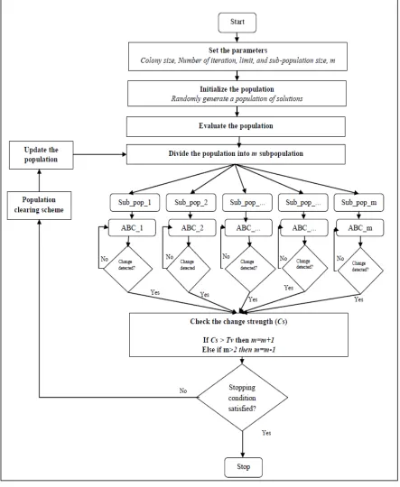
sub-population utilises an ABC algorithm. If a change in the problem is detected, the algorithm calculates the change strength to update the sub-population size and checks the stopping condition. If the specified stopping condition (we set this as a maximum number of fitness evaluations) has been reached, the algorithm terminates and the best solution is returned. Otherwise, the algorithm merges all the sub-populations, updates the population, runs the clearing method, re-divides the population into m sub-populations and starts a new iteration.
The main steps are described in further detail below:
- Step 1: Set parameters. The main parameters of Multi-pop-ABC are initialised. The algorithm has five parameters. Four of them are the same as the basic ABC. These are: the maximum number of iterations (MaxIt), population size (Ps), number of bees (Sbees), and the limit parameter (Lit). The fifth parameter is the sub-population size (m), which represents the number of sub-populations (Ps/m). Initially, m=2 and during the search process, it is either decreased or increased.
1- Step 2: Initialise the population of solutions. Same as Step 2 in the basic ABC, Section
2.1.
2- Step 3: Evaluate the population of solutions. Same as Step 3 in the basic ABC, Section
2.1.
3- Step 4: Divide the population. The population of solutions is divided into m sub-populations (Ps/m). Each sub-population is assigned to explore a different area of the search space. These sub-populations interact with each other through merging and re-dividing every time a change in the environment is detected. Each solution in the population is randomly assigned to a sub-population. The number of sub-populations m is either increased or decreased based on the environment change strength. The initial value of m is set to two (m=2) and it is updated during the search.
4- Step 5: Assign ABC to each sub-population. Each sub-population has its own ABC
population of solutions and iteratively calls the following until the stopping condition is satisfied (the algorithm stops when a change in the environment is detected):
i. Employee bees. Same as Step 4 in the basic ABC, Section 2.1.
ii. Onlooker bees. Same as Step 5 in the basic ABC, Section 2.1.
iii. Scout bees. Same as Step 6 in the basic ABC, Section 2.1.
5- Step 6: Check the change strength. This step is activated when a change in the environment is detected. Its main role is to update the number of sub-populations based on the environment change strength. It first calculates the objective function of the best solution before and after the environment change as follows:
Cs f(best_before) f(best_after) (4)
where Cs is the change strength, f(best_before) is the quality of the best solution before the environment change and f(best_after) is the quality of the best solution after the environment change. If the Cs is less than the defined threshold (Tv) and m is greater than 2, the number of sub-populations m is decreased as the algorithm needs to be more exploitive than explorative (m=m-1). Otherwise, m is increased by one with the aim of increasing the exploration aspect of the search (m=m+1). It should be noted that when m is an odd number, the extra solution is randomly assigned to one of the sub-populations.
6- Step 7: Check the stopping condition. This step checks the termination criterion of the
search process. In this work, it is set as a maximum number of fitness evaluations in line with previous works. If the specified stopping condition is reached, the search process stops and returns the best solution. Otherwise, the algorithm performs the following processes:
i. Population clearing scheme: This scheme calculates the similarity between
solutions are similar if they have the same values in all the cells of both solutions. If two or more solutions are similar, these solutions are deleted and replaced with randomly generated ones.
ii. Population update: All sub-populations are merged to form one population.
Figure 1. The proposed Multi-pop-ABC
3. Experimental Setup
3.1 The Moving Peak Benchmark
The moving peak benchmark (MPB) is a maximization dynamic continuous optimization problem proposed by [9], [25], and has been commonly used as a testbed for the performance of optimisation algorithms. MPB consists of a set of peaks that move over the problem landscape. It takes the given solution as an input and returns the value of the highest peak. The returned value represents the quality of this solution. MPB can be mathematically expressed as follows:
D j ij j i i i t X t x t W t H p t x F 1 2 ,..., 1 )) ( ) ( ( ) ( 1 ) ( max ) ,
( (5)
where F(x, t) is the quality of solution x at time t, p is the number of peaks, D is the problem dimension (number of decision variables where each variable has an upper and lower boundary (DB)), Hi (t) is the height of peak i, Wi (t) is the width of peak i, and Xij is the jth element of the location of peak i. Note that Equation (5) is a stationary optimization problem. Thus, to change it to a dynamic problem, MPB randomly shifts the position of all peaks by vector vi of a distance s (s is also known as the shift length that determines the severity
degree) as follows:
)) 1 ( ) 1 (( | ) 1 ( | )
( r v t
t v r s t v i i
i (6)
where
r
is a random vector, λ is the correlation between consecutive movements of a single peak that takes either “0” if the movement of peaks are completely uncorrelated or “1” if they move in the same direction. To make a fair comparison with existing algorithms, in this paper, we used λ=0 [6]. The change of height and width of a peak in a given solution can be mathematically expressed as follows:severity
height
t
H
t
H
i(
)
i(
1
)
_
(7)severity
width
t
W
t
W
i(
)
i(
1
)
_
(8)) ( ) 1 )( ( )
(t X t t v t
Xi i i (9)
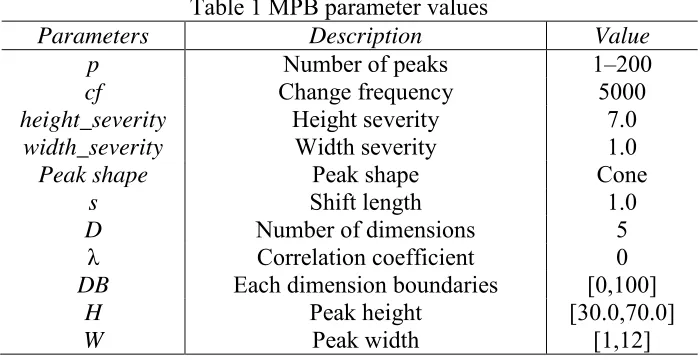
[image:15.595.128.478.190.370.2]The change frequency (cf) occurs every 5,000 fitness evaluations [9]. The parameter values of all MPBs that have been used in our experiments are shown in Table 1 [25].
Table 1 MPB parameter values
Parameters Description Value
p Number of peaks 1–200
cf Change frequency 5000
height_severity Height severity 7.0
width_severity Width severity 1.0
Peak shape Peak shape Cone
s Shift length 1.0
D Number of dimensions 5
λ Correlation coefficient 0
DB Each dimension boundaries [0,100]
H Peak height [30.0,70.0]
W Peak width [1,12]
3.2 Evaluation Metric
To fairly compare the proposed ABC with existing algorithms, we use the same evaluation metric known as the offline error as suggested by [25]. This has also been used by other researchers. The offline error is calculated as follows:
g
i i g off
1 1
(10)
where g is the number of generations and Ω is the best performance since the last change at ith fitness evaluation.
3.3 Parameter Settings
population size (Ps), limit (Lit) and the change strength threshold (Tv). First, we fixed Lit to 30, Tv to 0.09 and changed Ps. Table 2 shows the offline error of various Ps values for 50 and 200 peaks. The best result is highlighted in bold. Next, we fixed Ps to 60, Tv to 0.09 and changed Lit as shown in Table 3. Finally, we fixed Ps to 60, Lit to 30 and changed Tv as shown in Table 4. The parameter settings of the proposed ABC that were used across all scenarios are presented in Table 5.
Table 2 The value of Ps parameter Ps value 50 peaks 200 peaks
20 0.95669 2.70215 40 0.319632 1.8935 60 0.5810 0.34865
80 0.576911 1.15134
Table 3 The value of Lit parameter Lit value 50 peaks 200 peaks
10 1.03474 1.18977 20 1.27535 1.70215 30 1.29851 0.24824
40 1.841891 1.28967
Table 4 The value of Tv parameter Tv value 50 peaks 200 peaks
0.03 0.95669 1.89663 0.05 0.96573 1.08053
0.07 0.89978 1.37518 0.09 1.23491 1.77956
Table 5 The parameter settings of the proposed ABC
# Parameter Value
1- Maximum number of iterations (MaxIt)
50,000 fitness evaluations 2- Population size (Ps) 60
3- Limit parameter (Lit) 30 4- Change strength threshold (Tv) 0.05
4. Results
compared with state of the art methods. In the third experiment, the results of Multi-pop-ABC on well-known test functions are compared with state of the art methods.
4.1 Results comparison of Multi-pop-ABC and the basic ABC
This section aims to verify the effectiveness of the additional components that we have added to the basic ABC. Specifically, the objective is to investigate the impact of the proposed enhancements on the performance of the basic ABC when dealing with DOPs. Four different algorithms were derived as follows:
- Multi-pop-ABC: the proposed ABC that utilises the adaptive multi-population and population clearing scheme
- Multi-pop-ABC1: same as above but without the population clearing scheme
- Multi-pop-ABC2: same as above but uses a fixed number of sub-populations and without the population clearing scheme. The sub-populations were fixed to be the same as [26]
- ABC: basic ABC algorithm.
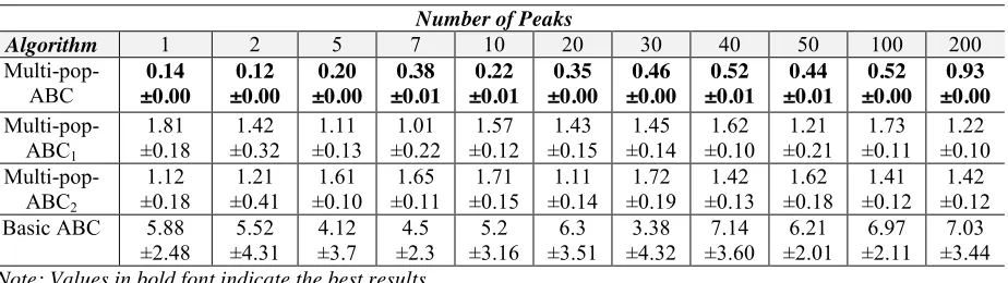
[image:17.595.74.536.628.758.2]The computational comparisons of Multi-pop-ABC, Multi-pop-ABC1, Multi-pop-ABC2 and basic ABC are presented in Table 6. The comparison is in terms of the offline error, ± standard error for each number of peaks. The best results are highlighted in bold. The results clearly show the good performance of Multi-pop-ABC when compared to Multi-pop-ABC1, Multi-pop-ABC2 and basic ABC. Indeed, Multi-pop-ABC outperformed Multi-pop-ABC1, Multi-pop-ABC2 and basic ABC on both the offline error and the standard error on all tested scenarios. The results demonstrate that the enhancements we made to the basic ABC improve the algorithmic performance.
Table 6 Results of the Multi-pop-ABC, Multi-pop-ABC1, Multi-pop-ABC2 and basic ABC
Number of Peaks
Algorithm 1 2 5 7 10 20 30 40 50 100 200
Multi-pop-ABC ±0.00 0.14
0.12 ±0.00
0.20 ±0.00
0.38 ±0.01
0.22 ±0.01
0.35 ±0.00
0.46 ±0.00
0.52 ±0.01
0.44 ±0.01
0.52 ±0.00
0.93 ±0.00
Multi-pop-ABC1
1.81
±0.18 ±0.32 1.42 ±0.13 1.11 ±0.22 1.01 ±0.12 1.57 ±0.15 1.43 ±0.14 1.45 ±0.10 1.62 ±0.21 1.21 ±0.11 1.73 ±0.10 1.22
Multi-pop-ABC2
1.12
±0.18 ±0.41 1.21 ±0.10 1.61 ±0.11 1.65 ±0.15 1.71 ±0.14 1.11 ±0.19 1.72 ±0.13 1.42 ±0.18 1.62 ±0.12 1.41 ±0.12 1.42 Basic ABC 5.88
±2.48
5.52 ±4.31
4.12 ±3.7
4.5 ±2.3
5.2 ±3.16
6.3 ±3.51
3.38 ±4.32
7.14 ±3.60
6.21 ±2.01
6.97 ±2.11
7.03 ±3.44
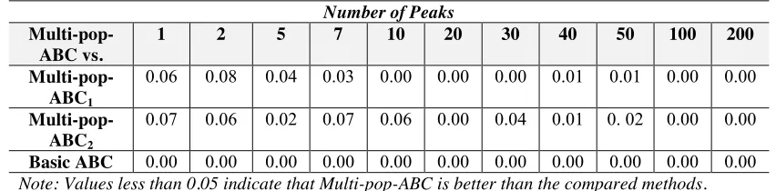
To further verify the results, we conducted a comparison between Multi-pop-ABC and each method separately. We used a Wilcoxon statistical test with a confidence level of 0.05. The p -values of Multi-pop-ABC against Multi-pop-ABC1, Multi-pop-ABC2 and basic ABC for each scenario is presented in Table 7. A value less than 0.05 indicates Multi-pop-ABC is superior (i.e. statistically different). As can be seen from Table 7, pop-ABC is superior to Multi-pop-ABC1, Multi-pop-ABC2 and basic ABC on 9 out of 11 tested scenarios (p < 0.05). The table also shows than on two scenarios (1 peak and 2 peaks) Multi-pop-ABC is not superior to Multi-pop-ABC1 and Multi-pop-ABC2. This can be attributed to the fact that these two scenarios are relatively easy to solve and thus all methods produce very good solutions. The results of the statistical test also demonstrate that the proposed enhancements have a positive impact and improve the search process.
Table 7 p-values of the of Multi-pop-ABC against other methods Number of Peaks
Multi-pop-ABC vs.
1 2 5 7 10 20 30 40 50 100 200
Multi-pop-ABC1
0.06 0.08 0.04 0.03 0.00 0.00 0.00 0.01 0.01 0.00 0.00
Multi-pop-ABC2
0.07 0.06 0.02 0.07 0.06 0.00 0.04 0.01 0. 02 0.00 0.00
Basic ABC 0.00 0.00 0.00 0.00 0.00 0.00 0.00 0.00 0.00 0.00 0.00 Note: Values less than 0.05 indicate that Multi-pop-ABC is better than the compared methods.
4.2 Comparison with state of the art methods
There are numerous methods that use different schemes to handle diversification, and which have been tested on MPB. In this section, we evaluate the performance of our algorithm by comparing it with several recently proposed algorithms taken from the scientific literature. The algorithms are:
- Multiswarms, exclusion, and anti-convergence in dynamic environments (mCPSO) [27].
- Multiswarms, exclusion, and anti-convergence in dynamic environments (mQSO) [27]
- Multiswarms, exclusion, and anti-convergence in dynamic environments (mQSO*) [27].
- Competitive population evaluation in a differential evolution algorithm for dynamic environments (CDE) [28].
- Differential evolution for dynamic environments with unknown numbers of optima (DynPopDE) [29].
- Dynamic function optimization with hybridized extremal dynamics (EO + HJ) [30] - A competitive clustering particle swarm optimizer for dynamic optimization problems
(CCPSO) [31].
- A novel hybrid adaptive collaborative approach based on particle swarm optimization and local search for dynamic optimization problems ( CHPSO(ES-NDS)) [32].
To ensure a fair comparison, we used the same stopping condition (50,000 fitness evaluations), the same change frequency (every 5,000 fitness evaluations) and the same evaluation metric (Offline error). We also used 11 MPB instances with a different number of peaks ranging between 1 to 200 peaks.
[image:19.595.69.537.664.749.2]The results of Multi-pop-ABC and the compared algorithms are presented in Table 8. The results in the table are in terms of offline error, ± standard error and computational times for each number of peaks. In the table, the symbol ‘-’ indicates that the scenario has not been tested. We indicate in bold the best obtained results. From Table 8, it can be seen that Multi-pop-ABC is superior to the other algorithms in most of the cases in terms of offline error. In particular, Multi-pop-ABC obtained new best results for 9 out of 11 tested MPB instances. Multi-pop-ABC was inferior on only two MPB instances: 1 peak and 2 peaks. Nevertheless, the results of Multi-pop-ABC for these two scenarios are very competitive, where it obtained the second best results. In terms of the standard error, Multi-pop-ABC produced a better standard error for 6 scenarios, being similar on 5 scenarios out of the 11 tested.
Table 8 Results of Multi-pop-ABC compared to the state of the art methods
Number of Peaks
Algorithm 1 2 5 7 10 20 30 40 50 100 200
Multi-pop-ABC ±0.00 0.14
8.11
0.12 ±0.00
9.10
0.20 ±0.00
10.20
0.38 ±0.01
10.63
0.22 ±0.01
11.12
0.35 ±0.00
13.75
0.46 ±0.00
15.13
0.52 ±0.01
17.17
0.44 ±0.01
20.23
0.52 ±0.00
28.64
0.93 ±0.00
56.48 mCPSO 4.93
mQSO 5.07
±0.17 ±0.23 3.47 ±0.07 1.81 ±0.07 1.77 ±0.06 1.80 ±0.07 2.42 ±0.07 2.48 ±0.07 2.55 ±0.06 2.50 ±0.04 2.36 ±0.03 2.26 mCPSO* 4.93
±0.17
3.36 ±0.26
2.07 ±0.11
2.11 ±0.11
2.05 ±0.07
2.95 ±0.08
3.38 ±0.11
3.69 ±0.11
3.68 ±0.11
4.07 ±0.09
3.97 ±0.08 mQSO* 5.07
±0.17 ±0.23 3.47 ±0.07 1.81 ±0.07 1.77 ±0.06 1.75 ±0.07 2.74 ±0.11 3.27 ±0.08 3.60 ±0.11 3.65 ±0.08 3.93 ±0.07 3.86
CDE - - - - 0.92
±0.07 - - - -
DynPopDE - - 1.03
±0.13 - ±0.07 1.39 - - - ±0.06 2.10 ±0.05 2.34 ±0.05 2.44 EO + HJ 7.08
±1.99
- - - 0.25
±0.10 0.39 ±0.10
0.49 ±0.09
0.56 ±0.09
0.58 ±0.09
0.66 ±0.07
-
CCPSO 0.09
±0.00 ±0.00 0.09 ±0.01 0.25 ±0.03 0.53 ±0.06 0.75 ±0.08 1.21 ±0.07 1.40 ±0.08 1.47 ±0.09 1.50 ±0.09 1.76 -
CHPSO(ES-NDS) 0.19 ± 0.00 - 0.44 ±0.02 - 0.64 ±0.02 ±0.01 0.91 0.99 ±0.01 1.02 ±0.01 1.03 ±0.01 1.04 ±0.01 1.01 ±0.00
Note: Values in bold font indicate the best results.
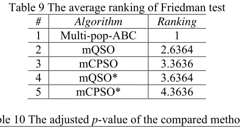
[image:20.595.69.534.69.263.2]To further verify the effectiveness of the proposed Multi-pop-ABC, we statistically compare it with other methods. We followed the procedure described in [33]. First, Friedman test and Iman and Davenport statistical tests with 0.05 confidence levels are carried out to detect if there is a difference between the results of Multi-pop-ABC and other methods. It should be noted that only those methods that were tested on all scenarios were considered for this test. Both the Friedman test and Iman and Davenport tests returned p-values (0.000009 and 0.000000009061) less than 0.05 indicating the compared results are statistically different. We next conducted a Friedman test to obtain rankings, and Holm and Hochberg post-hoc tests. The ranking value for each method obtained by a Friedman test is presented in Table 9 (the lower the better), where Multi-pop-ABC obtained the first rank followed by mQSO second rank, mCPSO third rank, mQSO* fourth rank and mCPSO* fifth rank. Consequently, Multi-pop-ABC will be the controlling method for the Holm and Hochberg post-hoc tests. The p -values of Holm and Hochberg tests are shown in Table 10. From the table, one can see that Multi-pop-ABC is statistically better than the compared methods on both Holm and Hochberg tests in which all the obtained p-values are less than 0.05.
Table 9 The average ranking of Friedman test
# Algorithm Ranking
1 Multi-pop-ABC 1
2 mQSO 2.6364
3 mCPSO 3.3636
4 mQSO* 3.6364
5 mCPSO* 4.3636
[image:20.595.179.422.623.752.2]1 mCPSO* 0.000001 0.000002 0.000002
2 mQSO* 0.000092 0.000276 0.000276
3 mCPSO 0.000455 0.00091 0.00091
4 mQSO 0.015219 0.015219 0.015219
The above results reveal that, in most of the tested scenarios, the proposed Multi-pop-ABC is better than the compared methods. These results are supported by statistical tests.
We hypothesise that several key features contribute to the high performance of the proposed algorithm (Multi-pop-ABC) on the dynamic problem. These can be summarised as follows:
- Multi-population: This feature is beneficial for maintaining the diversity of solutions in the population during the search process.
- Adaptive number of sub-populations: This feature helps the algorithm in changing the solution distribution over the search landscape to get better diversification and intensification based on the problem change strength.
- Population clearing scheme: This feature helps avoid having similar solutions within the population in order to further add to the diversification.
4.3 Comparison with state-of-the-art approaches on test functions
In this section, we evaluate our proposed algorithm based on other well-known ten test functions. The tested functions are widely used by researchers [34-37]. These functions are:
x
f
1 = ni 1xi
2 [-100, 100]n
x
f
2 = n ii i n
i 1 x 1x [-10, 10]
n
x
f
3 = 1 i 1 2i x n
i
j [-100, 100]n
x
f
4 = maxi{xi,1 i n} [-100, 100]n
x
f
5 = 11100 1 2 2 12n
i xi xi xi [-30, 30]
n
x
f
6 = 1 4 0,1random ix
n
i i [-1.28, 1.28]
x
f
7 = n ii 1 xisin x [-500, 500]
n
x
f
8 = ni 1 xi xi
2 10cos 2 10 [-5.12, 5.12]n
x
f
9 = x en x
n
n
i i
n
i i cos 2 20
1 exp 1
2 . 0 exp
20 1 2 1 [-32, 32]n
x
f
10 = cos 14000 1
1 1
2
i x
x n i
i n
i i [-600, 600]
n
Ta ble 11 M ea n, th e stand ard de viation (S D) o f f un cti ons wit
h 30 dim
Table 12 Mean, the standard deviation (SD) of functions with 50 dimension.
F ABC PS-ABC PS-ABCII Multi-pop-ABC
Dim Mean SD Mean SD Mean SD Mean SD
f1 50 1.1483 x 10⁻⁵ 1.6272 x 10⁻⁵
0 0 0 0 0 0
f2 50 2.8511 x 10⁻³ 1.3944 x 10⁻³
0 0 0 0 0 0
f3 50 4.6422 x 10⁴ 6.9821 x 10³ 3.0638 x 10³ 3.4739 x 10³ 1.2539 x 10⁵ 2.1047 x 10⁴
2.1041 x 10³ 2.0893 x 10³
f4 50 5.6020 x 101 5.1905 1.8782 x 101 5.7908
0 0 0 0
f5 50 3.7224 x 101 3.6453 x 101 3.1451 x 101 2.9224 x 101 4.8504 x 101 1.3535 x 10⁻¹
2.2310 x 101 2.1102 x 101
f6 50 4.2726 x 10⁻¹ 8.2393 x 10⁻² 5.7802 x 10⁻² 1.6469 x 10⁻² 5.4388 x 10⁻⁴ 6.4470 x 10⁻⁴ 2.1847 x 10⁻⁴ 3.2711 x 10⁻⁴
f7 50 -19359.1 3.1097 x 10² -20893.4 7.9224 x 101 -19414.1 3.3738 x 10²
-26893.4 7.8394 x 101
f8 50 8.1857 2.4195 0 0 0 0 0 0
f9 50 4.0637 x 10⁻² 3.2467 x 10⁻² 8.8817 x 10⁻¹⁶ 0 8.8817 x 10⁻¹⁶ 0
0 0
10 50 9.9977 x 10⁻³ 1.1718 x 10⁻²
0 0 0 0 0 0
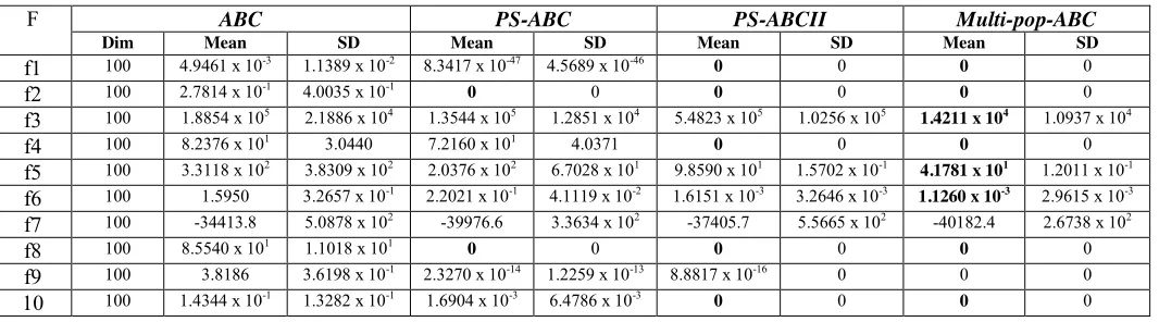
Table 13 Mean, the standard deviation (SD) of functions with 100 dimension.
F ABC PS-ABC PS-ABCII Multi-pop-ABC
Dim Mean SD Mean SD Mean SD Mean SD
f1 100 4.9461 x 10⁻³ 1.1389 x 10⁻² 8.3417 x 10-47 4.5689 x 10-46
0 0 0 0
f2 100 2.7814 x 10⁻¹ 4.0035 x 10⁻¹
0 0 0 0 0 0
f3 100 1.8854 x 10⁵ 2.1886 x 10⁴ 1.3544 x 10⁵ 1.2851 x 10⁴ 5.4823 x 10⁵ 1.0256 x 10⁵
1.4211 x 10⁴ 1.0937 x 10⁴
f4 100 8.2376 x 101 3.0440 7.2160 x 101 4.0371
0 0 0 0
f5 100 3.3118 x 10² 3.8309 x 10² 2.0376 x 10² 6.7028 x 101 9.8590 x 101 1.5702 x 10⁻¹
4.1781 x 101 1.2011 x 10⁻¹
f6 100 1.5950 3.2657 x 10⁻¹ 2.2021 x 10⁻¹ 4.1119 x 10⁻² 1.6151 x 10⁻³ 3.2646 x 10⁻³
1.1260 x 10⁻³ 2.9615 x 10⁻³
f7 100 -34413.8 5.0878 x 10² -39976.6 3.3634 x 10² -37405.7 5.5665 x 10² -40182.4 2.6738 x 10²
f8 100 8.5540 x 101 1.1018 x 101
0 0 0 0 0 0
f9 100 3.8186 3.6198 x 10⁻¹ 2.3270 x 10⁻¹⁴ 1.2259 x 10⁻¹³ 8.8817 x 10⁻¹⁶ 0 0 0
10 100 1.4344 x 10⁻¹ 1.3282 x 10⁻¹ 1.6904 x 10⁻³ 6.4786 x 10⁻³
0 0 0 0
5. Conclusion
[image:24.595.32.565.295.443.2]also produced better results than the state of the art methods on many scenarios, indicating that the proposed algorithm is an effective method for the DOP.
Acknowledgements
This work was supported by the Ministry of Education, Malaysia (FRGS/1/2015/ICT02/UKM/01/2) and the Universiti Kebangsaan Malaysia (DIP-2012-15).
References
1. Jin, Y. and J. Branke, Evolutionary optimization in uncertain environments-a survey. IEEE Transactions on Evolutionary Computation, 2005. 9(3): p. 303-317.
2. Nguyen, T.T., S. Yang, and J. Branke, Evolutionary dynamic optimization: A survey of the state of the art. Swarm and Evolutionary Computation, 2012. 6: p. 1-24.
3. Li, C., T.T. Nguyen, M. Yang, S. Yang, and S. Zeng, Multi-population methods in unconstrained continuous dynamic environments: The challenges. Information Sciences, 2015. 296: p. 95-118.
4. Hatzakis, I. and D. Wallace. Dynamic multi-objective optimization with evolutionary algorithms: a forward-looking approach. in Proceedings of the 8th annual conference on Genetic and evolutionary computation. 2006. p. 1201-1208. ACM.
5. Simões, A. and E. Costa. Improving prediction in evolutionary algorithms for dynamic environments. in Proceedings of the 11th Annual conference on Genetic and evolutionary computation. 2009. p. 875-882. ACM.
6. Branke, J. and D.C. Mattfeld, Anticipation and flexibility in dynamic scheduling. International Journal of Production Research, 2005. 43(15): p. 3103-3129.
7. Cruz, C., J.R. González, and D.A. Pelta, Optimization in dynamic environments: a survey on problems, methods and measures. Soft Computing, 2011. 15(7): p. 1427-1448.
8. Branke, J. Memory enhanced evolutionary algorithms for changing optimization problems. in In Congress on Evolutionary Computation CEC99. 1999. 3:1875-1882. 9. Branke, J., Evolutionary optimization in dynamic environments. Vol. 3. 2012:
Springer Science & Business Media.
10. Yang, S. On the design of diploid genetic algorithms for problem optimization in dynamic environments. in IEEE Congress on Evolutionary Computation CEC 2006. pp. 1362-1369.
11. Daneshyari, M. and G.G. Yen. Dynamic optimization using cultural based PSO. in IEEE Congress on Evolutionary Computation CEC 2011 pp. 509-516.
12. Grefenstette, J.J. Evolvability in dynamic fitness landscapes: A genetic algorithm approach. in IEEE Congress on Evolutionary Computation CEC 1999. Vol. 3, pp.2031 -2038 1999.
13. Ursem, R.K. Multinational GAs: Multimodal Optimization Techniques in Dynamic Environments. in In GECCO, pp. 19-26. 2000.
14. Branke, J., T. Kaußler, C. Schmidt, and H. Schmeck, A multi-population approach to dynamic optimization problems. Adaptive computing in design and manufacturing,2000:, 2000: p. 299-308.
16. Mendes, R. and A.S. Mohais. DynDE: a differential evolution for dynamic optimization problems. in IEEE Congress on Evolutionary Computation CEC 2005 vol. 3, pp. 2808-2815.
17. Li, C. and S. Yang. Fast multi-swarm optimization for dynamic optimization problems. in Fourth International Conference on Natural Computation, 2008. ICNC'08. . vol. 7, pp. 624-628. IEEE.
18. Yang, S. and C. Li, A clustering particle swarm optimizer for locating and tracking multiple optima in dynamic environments. IEEE Transactions on Evolutionary Computation, , 2010. 14(6): p. 959-974.
19. Turky, A.M. and S. Abdullah, A multi-population electromagnetic algorithm for dynamic optimisation problems. Applied Soft Computing, 2014. 22(1): p. 474-482.
20. Turky, A.M. and S. Abdullah, A multi-population harmony search algorithm with external archive for dynamic optimization problems. Information Sciences, 2014.
272(1): p. 84-95.
21. Sharifi, A., J.K. Kordestani, M. Mahdaviani, and M.R. Meybodi, A novel hybrid adaptive collaborative approach based on particle swarm optimization and local search for dynamic optimization problems. Applied Soft Computing, 2015. 32(1): p.
432-448.
22. Li, C., T.T. Nguyen, M. Yang, S. Yang, and S. Zeng, Multi-population methods in unconstrained continuous dynamic environments: The challenges. Information Sciences, 2015. 296(1): p. 95-118.
23. Karaboga, D., An idea based on honey bee swarm for numerical optimization. 2005, Technical report-tr06, Erciyes university, engineering faculty, computer engineering department.
24. Karaboga, D. and B. Basturk, A powerful and efficient algorithm for numerical function optimization: artificial bee colony (ABC) algorithm. Journal of global optimization, 2007. 39(3): p. 459-471.
25. Branke, J. and H. Schmeck, Designing evolutionary algorithms for dynamic optimization problems, in Advances in evolutionary computing. 2003, Springer. p. 239-262.
26. Branke, J., T. Kaußler, C. Smidt, and H. Schmeck, A multi-population approach to dynamic optimization problems, in Evolutionary Design and Manufacture. 2000, Springer. p. 299-307.
27. Blackwell, T. and J. Branke, Multiswarms, exclusion, and anti-convergence in dynamic environments. IEEE Transactions on Evolutionary Computation, 2006. 10(4): p. 459-472.
28. Du Plessis, M.C. and A.P. Engelbrecht, Using competitive population evaluation in a differential evolution algorithm for dynamic environments. European Journal of Operational Research, 2012. 218(1): p. 7-20.
29. Du Plessis, M.C. and A.P. Engelbrecht, Differential evolution for dynamic environments with unknown numbers of optima. Journal of Global Optimization, 2013. 55(1): p. 73-99.
30. Moser, I. and R. Chiong, Dynamic function optimisation with hybridised extremal dynamics. Memetic Computing, 2010. 2(2): p. 137-148.
31. Nickabadi, A., M.M. Ebadzadeh, and R. Safabakhsh, A competitive clustering particle swarm optimizer for dynamic optimization problems. Swarm Intelligence, 2012. 6(3): p. 177-206.
search for dynamic optimization problems. Applied Soft Computing, 2015. 32: p.
432-448.
33. García, S., A. Fernández, J. Luengo, and F. Herrera, Advanced nonparametric tests for multiple comparisons in the design of experiments in computational intelligence and data mining: Experimental analysis of power. Information Sciences, 2010. 180(10): p. 2044-2064.
34. Li, G., P. Niu, Y. Ma, H. Wang, and W. Zhang, Tuning extreme learning machine by an improved artificial bee colony to model and optimize the boiler efficiency. Knowledge-Based Systems, 2014. 67: p. 278-289.
35. Cui, H., J. Feng, J. Guo, and T. Wang, A novel single multiplicative neuron model trained by an improved glowworm swarm optimization algorithm for time series prediction. Knowledge-Based Systems, 2015. 88: p. 195-209.
36. Mitić, M., N. Vuković, M. Petrović, and Z. Miljković, Chaotic fruit fly optimization algorithm. Knowledge-Based Systems, 2015. 89: p. 446-458.
37. Yeh, W.-C., An improved simplified swarm optimization. Knowledge-Based Systems,
An Adaptive Multi-population Artificial Bee Colony Algorithm for Dynamic Optimisation Problems
Shams K. Nseef1, Salwani Abdullah1, Ayad Turky2 and Graham Kendall3,4
1Data Mining and Optimisation Research Group, Centre for Artificial Intelligence Technology, Universiti Kebangsaan Malaysia, 43600 Bangi, Selangor, Malaysia.
E-mail: [email protected]; [email protected] 2Swinburne University of Technology, Melbourne, Victoria, Australia
E-mail: [email protected]
3University of Nottingham Malaysia Campus, Semenyih, Malaysia
4ASAP Research Group, University of Nottingham, Nottingham, United Kingdom
Email: [email protected]; [email protected]
Abstract
Recently, interest in solving real-world problems that change over the time, so called dynamic optimisation problems (DOPs), has grown due to their practical applications. A DOP requires an optimisation algorithm that can dynamically adapt to changes and several methodologies have been integrated with population-based algorithms to address these problems. Multi-population algorithms have been widely used, but it is hard to determine the number of populations to be used for a given problem. This paper proposes an adaptive multi-population artificial bee colony (ABC) algorithm for DOPs. ABC is a simple, yet efficient, nature inspired algorithm for addressing numerical optimisation, which has been successfully used for tackling other optimisation problems. The proposed ABC algorithm has the following features. Firstly it uses multi-populations to cope with dynamic changes, and a clearing scheme to maintain the diversity and enhance the exploration process. Secondly, the number of sub-populations changes over time, to adapt to changes in the search space. The moving peaks benchmark DOP is used to verify the performance of the proposed ABC. Experimental results show that the proposed ABC is superior to the ABC on all tested instances. Compared to state of the art methodologies, our proposed ABC algorithm produces very good results.
Keywords: dynamic optimisation, artificial bee colony algorithm, adaptive multi-population
method, meta-heuristics
1. Introduction
Many real-world optimisation problems have the characteristic of changing over time in terms of decision variables, constraints and the objective function [1], [2]. These problems
*Revised Manuscript (Clean Version)
are referred to as dynamic optimisation problems (DOPs) in the scientific literature. A DOP requires an optimisation algorithm that can dynamically adapt to the changes and track the optimum solution during the execution of the algorithm [2]. Given their practical applications and complexity, DOPs have attracted a lot of research attention. Population-based algorithms, which are a set of methodologies that utilise a population of solutions distributed over the search space, have attracted particular attention, due to their good performance [1], [2]. A key challenge in developing an optimisation algorithm for DOPs is how to maintain population diversity during the search process in order to keep track of landscape changes [3]. Several interesting diversity schemes have been developed in order to improve the search capability of population-based algorithms so that they can adapt effectively to the problem as it changes.
training process does not capture real world scenarios and there is a possibility of training errors due to lack of training data [7], [2].
Memory based methodologies aim to maintain diversity. They use a memory with a fixed size to store some of promising solutions that are captured during the search process. When a change is detected, the stored solutions will be reinserted into the current population and the population will be filtered to include only the best solutions. Examples of memory based methodologies can be found in [8], [9], [10], [11]. These methodologies have worked well when the dynamic problems are periodical or cyclic. The drawback is that they have parameter sensitivities that need to be determined in advance, and most real world problems are not cyclic in nature.
very good results when tested on the MPB. Turky and Abdullah [19] proposed a multi-population electromagnetic algorithm for DOPs. The proposed algorithm divides the population into several sub-populations to simultaneously explore and exploit the search process. The algorithm was tested on MPB problems and obtained very good results when compared to other population diversity mechanisms. The same authors [20] also presented a multi-population harmony search algorithm for the DOP. The population is divided into sub-populations. Each sub-population is responsible for either exploring or exploiting the search space. An external archive is utilised to track the best solutions found so far, which are used to replace the worst ones when a change is detected. The results show that this algorithm produces good results when compared to other methods. Sharifi et al. [21] proposed a hybrid PSO and local search algorithm for DOPs. The algorithm utilises a fuzzy social-only model to locate the peaks. The results show that this algorithm can produce very good results for MPB problems. In Li et al. [22] comprehensive experimental analysis was reported on the performance of a multi-population method with various algorithms in relation to DOPs. The authors concluded that the multi-population method is able to deal effectively with various DOPs and has the ability to maintain population diversity. It is also able to help the search in locating a new area through a divide and merge process and information exchange. The authors also highlighted several weaknesses of their method that relate to the number of sub-populations, the distribution of solutions and the reaction to problem changes.
Existing works on DOPs demonstrate that employing multi-population methods are the most effective method in maintaining population diversity. The features that make the multi-population methodologies popular are [3]: i) it divides the multi-population into sub-multi-populations, where the overall population diversity can be maintained since different populations can be located in different areas of the problem landscape, ii) it has the ability to search different areas simultaneously, enabling it to track the movement of the optimum, and iii) various single population-based algorithms can be integrated within multi-population methods.
divide the population into sub-populations, rather than focussing on diversification. To address these issues, this work proposes an adaptive multi-population artificial bee colony (ABC) algorithm for the DOP. The proposed ABC utilises a clearing scheme to remove redundant solutions in order to maintain diversity and enhance the exploration process. To efficiently track the landscape changes, the proposed ABC algorithm adaptively updates the number of sub-populations based on the problem change strength.
In this paper, the key objectives are:
i. To propose an artificial bee colony algorithm that utilises a multi-population and a
population clearing scheme to efficiently solve the dynamic optimisation problem.
ii. To propose an adaptive multi-population algorithm that updates the number of the
sub-populations based on the problem change strength.
iii. To test the performance of the proposed algorithm on dynamic optimisation problems
using different scenarios and compare the results with other methodologies.
We used the moving peaks benchmark DOP with a different number of peaks to evaluate the effectiveness of the proposed ABC. Results demonstrate that the proposed ABC performs better than a basic ABC on all tested scenarios. Compared to the state of the art method, the proposed ABC produces very good results for many instances.
2. The proposed algorithm
This section presents the basic artificial bee colony algorithm, as well as our proposed adaptive multi-population algorithm.
2.1 Basic artificial bee colony algorithm
quality (objective function) of the problem being addressed. The three types of bees work together in an iterative manner to improve the quality of the population of solutions (food sources). The pseudo-code of a basic ABC is shown in Algorithm 1 [24]. ABC first sets the main parameters, initializes the population of solutions and then evaluates them. Next, the main loop is executed in an attempt to solve the given optimisation problem by calling the employee bees, onlooker bees and scout bees until the stopping condition is satisfied.
Algorithm 1: The pseudo-code of basic ABC
Step 1: Set the parameter values
Step 2: Initialize the population of solutions
Step 3: Evaluate the population of solutions
while termination condition is not met do
Step 4: Employed Bees step
Step 5: Onlooker Bees step
Step 6: Scout Bees step
end while
The basic ABC has the following steps:
Step 1- Set ABC parameters. In this step the main parameters of ABC are initialized.
These include: the maximum number of iterations (MaxIt) which represents the stopping
condition of ABC, the number of solutions or population size (Ps) which represent how
many solutions will be generated, the total number of bees (Sbees) which is set to be
twice the size of Ps, where half of them are employee bees and the other half are
onlooker bees, the limit parameter (Lit), which is used to determine if the solution should
be replaced by a new one.
Step 2- Initialise the population of solutions. A set of solutions with size equal to Ps
are randomly generated as follows:
) ](
1 , 0
[ min
, max
, min
,
,j ij i j i j
i x Rand x x
x (1)
where i is the index of the solution, j is the current decision variable, Rand [0,1]
generates a random number between zero and one and min
,j i
x and ximax,j are the lower and
Step 3- Evaluate the population of solutions. The fitness (quality) of the generated solutions are calculated using the objective function. The objective function is problem dependent. The objective function used in this work is shown in Section 3.2.
Step 4- Employed bees. Each employee bee is sent to one food source (solution). Its
main role is to explore the neighbourhood of the current solution, seeking an improving
solution. A neighbourhood solution, v, is created by modifying the ith solution, x, as
follows:
)
( , ,
, ,
,j ij ij i j k j
i x x x
v (2)
where k is a randomly selected solution from Ps and Φ is a random number between [-1,
1]. The generated neighbourhood solution will be replaced with current solution if it has better fitness.
Step 5- Onlooker bees. Onlooker bees seek to improve the current population of
solutions by exploring their neighbourhood using Equation (2), the same as the employee bee. The difference is that onlooker bees select the solutions probabilistically based on their fitness values as follows:
Ps
j
i i
fitnessj fitness p
1 (3)
That is, the solution with the higher fitness has a higher chance of being selected (i.e. roulette wheel selection). Onlooker bees use a greedy selection mechanism, where the better solution in terms of fitness is selected.
Step 6- Scout bees. This step is activated if both employed and onlooker bees cannot
improve the current solution for a number of consecutive iterations defined by the limit
parameter, Lit. This indicates that the current solution is not good enough to search its
solution using Equation (1) to replace the discarded one. This can help ABC to escape from a local optimum and explore a different area of the search space.
2.2 The proposed artificial bee colony algorithm
Existing works on DOPs have demonstrated that multi-population methods are state of the art, in that they outperform other methods on many scenarios. However, although multi-population methods have achieved success in solving DOPs, most of them use a fixed number of populations and the population diversity is maintained through the sub-population distribution. To address these issues, this work proposes an adaptive sub-population ABC (denoted as Multi-pop-ABC). In Multi-pop-ABC, three major modifications are added to the basic ABC. These are:
i. Multi-population method. To deal with DOP, the proposed ABC uses a multi-population
method to divide the population into several sub-populations. By using a multi-population method, the solutions are scattered over the search space instead of focusing on a specific area. Thus the algorithm can generate high quality solutions and track the problem changes.
ii. Adaptive scheme. To track the landscape changes that occur during the search process, the
proposed Multi-pop-ABC updates the number of sub-populations based on the strength of the problem change. That is the number of sub-populations is either decreased or increased during the search process. By using the proposed adaptive method, the number of sub-populations can be changed adaptively based on the strength of the environment changes, which helps the search track the optimum solution and also improves the diversification and exploration processes.
iii. Population clearing scheme. To ensure that the solutions are diverse enough, a population
clearing scheme is called when a change is detected to delete redundant solutions and replace them with new solutions. This scheme removes redundant solutions in order to maintain diversity and enhance the exploration process.
The flowchart of the proposed Multi-pop-ABC for DOPs is shown in Figure 1. It starts by setting the parameter values. It creates the population of solutions and then evaluates
sub-population utilises an ABC algorithm. If a change in the problem is detected, the algorithm calculates the change strength to update the sub-population size and checks the stopping condition. If the specified stopping condition (we set this as a maximum number of fitness evaluations) has been reached, the algorithm terminates and the best solution is returned. Otherwise, the algorithm merges all the sub-populations, updates the population, runs the
clearing method, re-divides the population into m sub-populations and starts a new iteration.
The main steps are described in further detail below:
- Step 1: Set parameters. The main parameters of Multi-pop-ABC are initialised. The
algorithm has five parameters. Four of them are the same as the basic ABC. These
are: the maximum number of iterations (MaxIt), population size (Ps), number of bees
(Sbees), and the limit parameter (Lit). The fifth parameter is the sub-population size
(m), which represents the number of sub-populations (Ps/m). Initially, m=2 and during
the search process, it is either decreased or increased.
1- Step 2: Initialise the population of solutions. Same as Step 2 in the basic ABC, Section
2.1.
2- Step 3: Evaluate the population of solutions. Same as Step 3 in the basic ABC, Section
2.1.
3- Step 4: Divide the population. The population of solutions is divided into m
sub-populations (Ps/m). Each sub-population is assigned to explore a different area of the
search space. These sub-populations interact with each other through merging and re-dividing every time a change in the environment is detected. Each solution in the
population is randomly assigned to a sub-population. The number of sub-populations m
is either increased or decreased based on the environment change strength. The initial
value of m is set to two (m=2) and it is updated during the search.
4- Step 5: Assign ABC to each sub-population. Each sub-population has its own ABC
population of solutions and iteratively calls the following until the stopping condition is satisfied (the algorithm stops when a change in the environment is detected):
i. Employee bees. Same as Step 4 in the basic ABC, Section 2.1.
ii. Onlooker bees. Same as Step 5 in the basic ABC, Section 2.1.
iii. Scout bees. Same as Step 6 in the basic ABC, Section 2.1.
5- Step 6: Check the change strength. This step is activated when a change in the
environment is detected. Its main role is to update the number of sub-populations based on the environment change strength. It first calculates the objective function of the best solution before and after the environment change as follows:
Cs f(best_before) f(best_after) (4)
where Cs is the change strength, f(best_before) is the quality of the best solution before
the environment change and f(best_after) is the quality of the best solution after the
environment change. If the Cs is less than the defined threshold (Tv) and m is greater
than 2, the number of sub-populations m is decreased as the algorithm needs to be more
exploitive than explorative (m=m-1). Otherwise, m is increased by one with the aim of
increasing the exploration aspect of the search (m=m+1). It should be noted that when m
is an odd number, the extra solution is randomly assigned to one of the sub-populations.
6- Step 7: Check the stopping condition. This step checks the termination criterion of the
search process. In this work, it is set as a maximum number of fitness evaluations in line with previous works. If the specified stopping condition is reached, the search process stops and returns the best solution. Otherwise, the algorithm performs the following processes:
i. Population clearing scheme: This scheme calculates the similarity between
solutions are similar if they have the same values in all the cells of both solutions. If two or more solutions are similar, these solutions are deleted and replaced with randomly generated ones.
ii. Population update: All sub-populations are merged to form one population.
iii. Re-divide the population: The population is re-divided into m sub-populations
Figure 1. The proposed Multi-pop-ABC
3. Experimental Setup