A Tensor Based Hyper-heuristic for Nurse Rostering
Shahriar Asta, Ender ¨Ozcan, Tim Curtois
ASAP, School of Computer Science, University of Nottingham, NG8 1BB, Nottingham, UK.
Abstract
Nurse rostering is a well-known highly constrained scheduling problem requir-ing assignment of shifts to nurses satisfyrequir-ing a variety of constraints. Exact algorithms may fail to produce high quality solutions, hence (meta)heuristics are commonly preferred as solution methods which are often designed and tuned for specific (group of) problem instances. Hyper-heuristics have emerged as general search methodologies that mix and manage a predefined set of low level heuristics while solving computationally hard problems. In this study, we describe an online learning hyper-heuristic employing a data sci-ence technique which is capable of self-improvement via tensor analysis for nurse rostering. The proposed approach is evaluated on a well-known nurse rostering benchmark consisting of a diverse collection of instances obtained from different hospitals across the world. The empirical results indicate the success of the tensor-based hyper-heuristic, improving upon the best-known solutions for four of the instances.
Keywords: Nurse Rostering, Personnel Scheduling, Data Science, Tensor Factorization, Hyper-heuristics.
1. Introduction
Hyper-heuristics are high level improvement search methodologies ex-ploring space of heuristics (Burke et al., 2013). According to (Burke et al., 2010c), hyper-heuristics can be categorized in many ways. A hyper-heuristic either selects from a set of available low level heuristics or generates new heuristics from components of existing low level heuristics to solve a problem,
Email addresses: [email protected](Shahriar Asta),[email protected](Ender
¨
leading to a distinction betweenselection andgeneration hyper-heuristics, re-spectively. Also, depending on the availability of feedback from the search process, hyper-heuristics can be categorized as learning and no-learning. Learning hyper-heuristics can further be categorized into online and offline methodologies depending on the nature of the feedback. Online hyper-heuristics learnwhile solving a problem whereas offline hyper-heuristics pro-cess collected data gathered from training instances prior to solving the prob-lem.
Nurse rostering is a highly constrained scheduling problem which was proven to be NP-hard (Karp, 1972) in its simplified form. Solving a nurse rostering problem requires assignment of shifts to a set of nurses so that 1) the minimum staff requirements are fulfilled and 2) the nurses’ contracts are respected (Burke et al., 2004). The general problem can be represented as a constraint optimisation problem using 5-tuples consisting of set of nurses, days (periods) including the relevant information from the previous and up-coming schedule, shift types, skill types and constraints.
according to a fixed probability (usually 0.5). More sophisticated accep-tance algorithms such as Simulated Annealing(SA), Late Accepaccep-tance (LA) and Great Deluge (GD) can be found in the scientific literature (Burke et al., 2013).
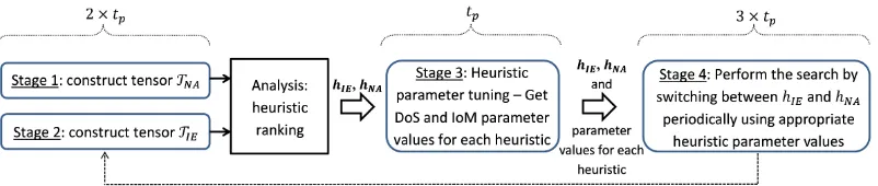
Our proposed approach consists of running the simple random heuristic selection strategy in four stages. In the first two stages, the acceptance mech-anism is NA, while in the second stage, we use IE as acceptance mechmech-anism. The trace of the hyper-heuristic in each stage is represented as a 3-rd order tensor. After each stage commences, the respective tensor is factorized which results in a score value associated to each heuristic. The space of heuristics is partitioned into two distinct sets, each representing a different acceptance mechanism (NA and IE respectively) and lower level heuristics associated to it. Subsequently, a hyper-heuristic is created which uses different ac-ceptance methods in an interleaving manner, switching between acac-ceptance methods periodically. In the third stage, the parameter values for heuristics is extracted by running the hybrid hyper-heuristic and collecting tensorial data similar to the first two stages. Subsequently, the hybrid hyper-heuristic equipped with heuristic parameter values is run for a specific time. The above mentioned procedure continues until the maximum allowed time is reached.
this study shows that tensor analysis can also play a parameter control role. The paper is organised as follows. Section 2 overviews the nurse rostering problem covering the problem definition, benchmarks in the area and related work. An introduction to tensor analysis is given in Section 3 where tensor representation of data, its advantages along with techniques widely employed to analyse tensorial data are explained. A detailed account of the proposed approach is provided in Section 4. The settings used in our experiments and the results of these experiments are laid out in Sections 5.1 and 5 respectively. Finally, concluding remarks and plans towards future work are discussed in Section 6.
2. Nurse Rostering
In this section, we define the nurse rostering problem dealt with. Addi-tionally, an overview of related work is provided.
2.1. Problem Definition
The constraints in the nurse rostering problem can be grouped into two categories: (i) those that link two or more nurses and (ii) those that only apply to a single nurse. Constraints that fall into the first category include the cover (sometimes called demand) constraints. These are the constraints that ensure a minimum or maximum number of nurses are assigned to each shift on each day. They are also specified per skill/qualification levels in some instances. Another example of a constraint that would fall into this category would be constraints that ensure certain employees do or do not work together. Although these constraints do not appear in most benchmark instances (including those used here), they do occasionally appear in practise to model requirements such as training/supervision, carpooling, spreading expertise etc. The second group of constraints model the requirements on each nurse’s individual schedule. For example, the minimum and maximum number of hours worked, permissible shifts, shift rotation, vacation requests, permissible sequences of shifts, minimum rest time and so on.
different organisations have different working regulations which have usually been defined by a combination of national laws, organisational and union requirements and worker preferences. To be able to model this variety, in (Burke and Curtois, 2014) a regular expression constraint was used. Using this domain specific regular expression constraint allowed all the nurse spe-cific constraints found in these benchmarks instances to be modelled. The model is given below.
Sets
E = Employees to be scheduled, e∈E T = Shift types to be assigned, t∈T
D = Days in the planning horizon, d∈ {1,· · · |D|}
Re = Regular expressions for employee e, r∈Re We = Workload limits for employee e, w∈We
Parameters
rmax
er = Maximum number of matches of regular expression r in the work
schedule of employee e.
rmin
er = Minimum number of matches of regular expression r in the work
schedule of employee e.
aer = Weight associated with regular expression r for employee e.
vmax
ew = Maximum number of hours to be assigned to employee e within the
time period defined by workload limit w.
vmin
ew = Minimum number of hours to be assigned to employee e within the
time period defined by workload limit w.
bew = Weight associated with workload limit w for employee e.
smax
td = Maximum number of shifts of type t required on day d. smin
td = Minimum number of shifts of type t required on day d.
ctd = Weight associated with the cover requirements of shift typet on dayd.
Variables
xetd = 1 if employee e is assigned shift type t on day d, 0 otherwise.
ner = The number of matches of regular expression r in the work schedule of employee e.
pew = The number of hours assigned to employee e within the time period defined by workload limit w.
Constraints
Employees can be assigned only one shift per day.
X
t∈T
xetd ≤1, ∀e∈E, d∈D (1)
Objective Function
Minf(s) =
X
e∈E
4
X
i=1
fe,i(x) +
X
t∈T
X
d∈D
6
X
i=5
ft,d,i(x) (2a)
where
fe,1(x) =
X
e∈Re
max{0,(ner−rermax)aer} (2b)
fe,2(x) =
X
e∈Re
max{0,(rmin
er −ner)aer} (2c)
fe,3(x) =
X
w∈We
max{0,(pew−vewmax)bew} (2d)
fe,4(x) =
X
w∈We
max{0,(vewmin−pew)bew} (2e)
fe,5(x) =max{0,(smintd −qtd)ctd} (2f) fe,6(x) =max{0,(qtd−smax
td )ctd} (2g)
working days, or constraints on the number of weekends worked, or the num-ber of night shifts and so on. Equations 2d and 2e ensure that each nurse’s workload constraints are satisfied. For example, depending on the instance, there may be a minimum and maximum number of hours worked per week, or per four weeks, or per month or however the staff for that organisation are contracted. Finally, equations 2f and 2g represent the demand (some-time called cover) constraints to ensure there are the required number of staff present during each shift. Again, depending upon the instance, there may be multiple demand curves for each shift to represent, for example, the min-imum and maxmin-imum requirements as well as a preferred staffing level. The weights for the constraints are all instance specific because they represent the scheduling goals for different institutions.
2.2. Related Work
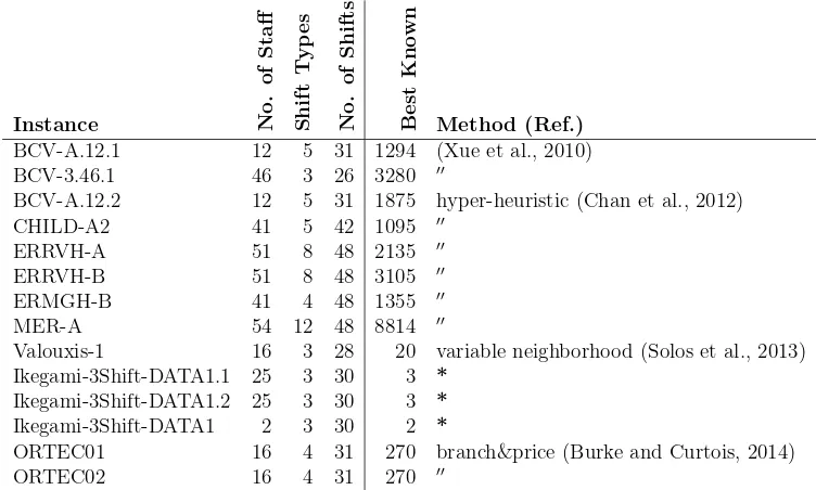
There are various benchmarks for nurse rostering. Curtois (2015) pro-vides a comprehensive public benchmark including the latest best known results together with the approaches yielding them. The characteristics of the benchmark instances used in the experiments are summarized in Table 1. There is a growing interest in challenges and the instances used during those challenges and resultant algorithms serve as a benchmark afterwards. The last nurse rostering competition was organised in 2010 (Haspeslagh et al., 2014) which consisted of three tracks where each track differed from oth-ers in maximum running time and size of instances. Many different algo-rithms have been proposed since then ((Valouxis et al., 2012), (L¨u and Hao, 2012), (Pillay and Rae, 2012), (Anwar et al., 2014), (Rae and Pillay, 2014), and more). Since it has been observed that the previous challenge did not impose much difficulty for the competitors (Burke and Curtois, 2014), other than developing a solution method in limited amount of time, a second chal-lenge has been organised which is ongoing 1
. In the second nurse rostering competition, the nurse rostering problem is reformulated as a multi-stage problem with fewer constraints where a solver is expected to deal with con-secutive series of time periods (weeks) and consider longer planning horizon. The remaining part of this section covers the state-of-the-art solution meth-ods applied to the benchmark instances from (Curtois, 2015) which are used during the experiments.
Instance No
.
o
f
S
ta
ff
S
h
if
t
T
y
p
e
s
N
o
.
o
f
S
h
if
ts
B
e
st
K
n
o
w
n
Method (Ref.)
BCV-A.12.1 12 5 31 1294 (Xue et al., 2010) BCV-3.46.1 46 3 26 3280 ′′
BCV-A.12.2 12 5 31 1875 hyper-heuristic (Chan et al., 2012) CHILD-A2 41 5 42 1095 ′′
ERRVH-A 51 8 48 2135 ′′
ERRVH-B 51 8 48 3105 ′′
ERMGH-B 41 4 48 1355 ′′
MER-A 54 12 48 8814 ′′
Valouxis-1 16 3 28 20 variable neighborhood (Solos et al., 2013) Ikegami-3Shift-DATA1.1 25 3 30 3 *
Ikegami-3Shift-DATA1.2 25 3 30 3 *
Ikegami-3Shift-DATA1 2 3 30 2 *
[image:8.595.118.494.301.527.2]ORTEC01 16 4 31 270 branch&price (Burke and Curtois, 2014) ORTEC02 16 4 31 270 ′′
In (M´etivier et al., 2009), the nurse rostering problem was identified as an over-constrained one and it is modelled using soft global constraints. A variant of Variable Neighbourhood Search (VNS), namely VNS/LDS+CP (Loudni and Boizumault, 2008), was used as a meta-heuristic to solve the problem instances. The proposed approach was tested on nine different in-stances from (Curtois, 2015). The experimental results show that the method is relatively successful, though the authors have suggested to use specific new heuristic for instances such as Ikegami to improve the performance of the algorithm.
(Xue et al., 2010) ????? This approach is the best on the BCV-A.12.1 and BCV-3.46.1 instances.
Glass and Knight (2010) proposed a method based on mixed integer lin-ear programming, solving four of the instances from (Curtois, 2015), namely,
ORTEC01, ORTEC02, GPost and GPost-B. The method is able to solve those
instances to optimality very quickly. The idea of implied penalties was in-troduced in the study. Employing implied penalties avoids accepting small improvements in the current rostering period at the expense of penalizing larger penalties on the next rostering period.
In (Burke et al., 2010d), a hybrid multi-objective model was presented to solve nurse rostering problems. The method is based on Integer Program-ming (IP) and Variable Neighbourhood Search (VNS). The IP method is used in the first phase of the algorithm to produce intermediary solutions considering all the hard constraints and a subset of soft constraints. The so-lution is further improved using the VNS method. The proposed approach is then applied to the ORTEC problem instances and compared to a commercial hybrid Genetic Algorithm (GA) and a hybrid VNS (Burke et al., 2008). The computational results show that the proposed approach outperforms both methods in terms of solution quality.
Chan et al. (2012) introduced a hyper-heuristic method inspired from pearl hunting and applied it to various nurse rostering instances. The pro-posed method is based on repeated intensification and diversification and can be described as a type of Iterated Local Search (ILS). Their experiments con-sisted of running the algorithm on various instances for several times, where each run is 24 CPU hours long. The algorithm discovered 6 new best-known results as illustrated in Table 1.
popu-lation of candidate solutions is generated. In the first phase of the algorithm, assigning nurses to working days is handled. Subsequent to this phase, in the second phase, assigning nurses to shift types is dealt with. Though, the proposed approach has been applied to few publicly available instances, the chosen instances are significantly different from one another. This is still the best approach producing the best known result for Valouxis-1 in the benchmark.
In (Burke and Curtois, 2014) a branch and price algorithm and an ejec-tion chain method was employed for solving the nurse rostering problem instances which were collected from thirteen different countries by the au-thors and made publically available from (Curtois, 2015). Branch and price method is based on the branch and bound technique with the difference that each node of the tree is a linear programming relaxation and is solved through column generation. The column generation method consists of two parts: the restricted master problem and the pricing problem. The former is solved using a linear programming method while the latter is using a dynamic programming approach. Some of the latest results and best-known solutions regarding the instances is provided by this study. Also, a general problem modelling scheme has been proposed in (Burke and Curtois, 2014) which is also adopted here due to its generality over many problem instances. This approach is the best on the ORTEC01 and ORTAC02 instances.
Numerous other approaches have been proposed to solve the nurse ros-tering problem. In (Azaiez and Al Sharif, 2005) the nurse rosros-tering problem was modelled using 0-1 Goal Programming Model. A shift sequence based approach was introduced in (Brucker et al., 2010). In (Burke et al., 2010b) a Scatter Search (SS) was presented to tackle the nurse rostering problem.
3. Tensor Analysis
data. Several recent studies dealt with this problem and proposed a solid remedy based on tensor analytic approaches ((Vasilescu and Terzopoulos, 2002),(Anandkumar et al., 2012) and (Acar et al., 2009)). These studies all show that tensorial representation and analytical approaches which come with it are capable of detecting patterns which where invisible to classical data mining approaches which have no regard for the natural dimensionality of the data.
Since their introduction, tensorial approaches have been employed and greatly contributed to a variety of research areas such as computer vision (Vasilescu and Terzopoulos, 2002), video processing (Krausz and Bauckhage, 2010), data compression (Wang et al., 2009), Signal Processing (Cichocki et al., 2014) and web mining (Acar et al., 2009), (Zou et al., 2015). Various prob-lems produce data of high order of dimensionality in nature and tensors, as multidimensional arrays, are fully suited to represent such data. For instance, video streams constitute a data which is three dimensional (pixel coordinates and time) or higher (when information such as audio, text, change of envi-ronment and etc are also considered). Such data can surely be presented as a three dimensional array which is commonly referred to as a nth-order tensor.
The order of a tensor indicates its dimensionality where each dimension of a tensor is referred to as a mode. For example, a tensor representing a video is a 3rd-order tensor.
The first step to extract latent patterns hidden within tensor data is to subject the tensor to factorization, say, decomposing the tensor into its basic factors. Several factorizations methods exist. Higher Order Singular Value Decomposition (HOSVD), Tucker decomposition, Parallel Factor de-composition and Non-negative Tensor Factorization (NTF) are among the most widely known factorization methods. HOSVD (Lathauwer et al., 2000) is a generalization of the Singular Value Decomposition (SVD) used in the Principal Component Analysis (PCA) method to higher dimensions. Tucker decomposition (Tucker, 1966c) decomposes a tensor into a set of matrices and a core tensor. Parallel Factor (a.k.a PARAFAC or CANDECOMP or CP) (Harshman, 1976) and Non-negative Tensor Factorization (NTF) (Shashua and Hazan, 2005) decompose a tensor into a sum of rank one tensors. Further information on tensors and applications and comparison between various factorization methods can be found in (Kolda and Bader, 2009).
boldface Euler script letters, boldface capital letters and boldface lower-case letters respectively (e.g.,T is a tensor,Mdenotes a matrix andvis a vector). Scalar values such as tensor, matrix and vector entries are indexed by lower-case letters. For example, tpqr is the (p, q, r) entry of a 3rd−order tensor
T.
3.1. CP Factorization
In this paper, following (Asta and ¨Ozcan, 2015), CP decomposition method is used for factorization. While Tucker decomposition is a generalization of the CP method, there are few advantages based on which the latter method is favoured over the former approach. Unlike the Tucker decomposition, the factors produced by the CP decomposition method are unique (under mild conditions)(Kolda and Bader, 2009). The tensor-based hyper-heuristic in this paper uses the scores achieved after factorization to rank heuristics. One should expect a reasonably high level of consistency between the heuris-tic rankings produced in various runs of the algorithm. Thus, uniqueness of the basic factors is a most crucial condition. Moreover, compared to Tucker decomposition, CP factorization produces easy to interpret basic factors. This is particularly desirable in the context of heuristics. Some applications (such as video, speech and text) produce easy-to-understand contents be-cause there is a certain semantic concept naturally associated with the data. This is not the case in the data produced by hyper-heuristics. Therefore, it is very desirable to choose a decomposition method which offers some level of simplicity in the process of interpreting the basic factors.
CP decomposition uses the Alternating Least Square (ALS) algorithm ((Carroll and Chang, 1970))S to decompose a tensor into its basic factors. That is, the original tensor T of sizeP ×Q×R is approximated by another tensor ˆT. The purpose of the ALS algorithm is to minimize the error differ-ence between the original tensor and the estimated tensor, denoted as ε as follows:
ε= 1
2||T −T ||ˆ 2
F (3)
where the subscript F refers to the Frobenious norm. That is:
||T −T ||ˆ 2F =
P
X
p=1
Q
X
q=1
R
X
r=1
tpqr −ˆtpqr2
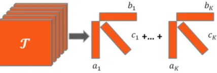
The approximated tensor contains the factors of the original tensor and can be expressed as a sum of rank one2
[image:13.595.199.413.235.307.2]tensors as in Equation 5 (this is also illustrated in Figure 1).
Figure 1: Factorizing a tensor toK components.
ˆ
T =
K
X
k=1
λk ak◦bk◦ck (5)
In Eq.5, λk ∈ R+, ak ∈ RP, bk ∈ RQ and ck ∈ RR for k = 1· · ·K, where K is the number of desired components. Each component k is of the form (λk ak ◦ bk ◦ ck) where λk is the weight of the component and the individual vectors (e.g. ak, bk and ck) are called factors. The number of components is set depending on the application. In this paper, we set the number of components to be K = 1. Therefore, the Equation 5 is reduced to the following equation.
ˆ
T =a◦b◦c (6)
The operator “◦” indicates an outer product. The outer product of three vectors produces a 3rd-order tensor. For instance, in Equation 6, ˆT is a 3rd
-order tensor which is obtained by the outer product of three vectors a,band
c. Subsequently, each tensor entry, denoted as ˆtpqr is computed through a simple multiplication like apbqcr.
Rather than using all the factors in the outer product which results in the approximated tensor ˆT, using only two of the factors in the outer product results in a structure which we refer to as the basic frame (Equation 7). It
2a tensor is of rank one when it can be written as the outer product ofN vectors. Many
was shown in several studies (e.g. (Krausz and Bauckhage, 2010)) that the basic frame exhibits very interesting phenomena.
B=a◦b (7)
For instance the basic frame B, which is actually a matrix, captures the hidden relationship between the first two modes of data. In other words, the matrix Bcontains score values which quantifies the relationship between the object pairs. For instance, in case of a video tensor and given that aand b
represent x and y values of pixel coordinates, the basic frame B quantifies the “level of interaction” between various pixel regions within a video.
Tensor factorization represents the original tensor in a concise form as can be seen from Equation 5. When it comes to mining the approximated data, the estimated tensor ˆT is also more generalizable and also increases the resistance to disruptions caused by data anomalies such as missing val-ues. Factorizing the tensor allow partitioning of the data into a set of more comprehensible sub-data which can be of specific use depending on the appli-cation according to various criteria. For example, in the field of computer vi-sion, (Kim and Cipolla, 2009) and (Krausz and Bauckhage, 2010) separately show that factorization of a 3rd-order tensor of a video sequence results in
some interesting basic factors. These basic factors reveal the location and functionality of human body parts which move synchronously.
4. Proposed Approach
the shifts in one or more randomly chosen employees’ schedule followed by a rebuilding procedure. These operators differ in the size of the perturbation they cause in the solution. Five local search heuristics, denoted by LS0,
LS1,LS2,LS3 andLS4 are also used where the first three heuristics are hill climbers and the remaining two are based on variable depth search. Also, three different crossover heuristics are used which are denoted byXO0,XO1 and XO2. The crossover operators are binary operators and applied to the current solution in hand and the best solution found so far (which is initially the first generated solution). More information on these heuristics can be found in (Curtois et al., 2009).
During the first two stages (line 2 and 3), two different tensors are con-structed. The tensor TN A is constructed by means of an SR-NA algorithm
and tensorTIE is constructed from the data collected from running an SR-IE
Figure 2: Overall approach with various stages.
Algorithm 1: Tensor-based hyper-heuristic
1 while t < Tmax do
2 (TN A) = ConstructTensor(h, NA, tp); 3 (TIE) = ConstructTensor(h, IE, tp); 4 (BN A,SN A) = Factorization(TN A,h); 5 (BIE,SIE) = Factorization(TIE,h);
6 (hN A,hIE) = Partitioning(BN A,BIE,SN A,SIE); 7 (P) = ParameterControl();
8 Improvement(hN A,hIE,P,SN A,SIE);
4.1. Tensor Analysis for Dynamic Low Level Heuristic Partitioning
During first and second stages, given an acceptance criteria (such as NA or IE), a hyper-heuristic with a simple random heuristic selection and the given acceptance methodology is executed. During the run, data, in the form of a tensor is collected. Hence the collected tensor data (TN A or TIE depending
on the acceptance criteria) is a 3rd-order tensor of size
R|h|×R|h|×Rt, where
|h|is the number of low level heuristics andtrepresents the number of tensor frames collected in a given amount of time. Each tensor is a collection of two dimensional matrices (M) which are referred to as tensor frames. A tensor frame is a two dimensional matrix of heuristic indices. Column indices in a tensor frame represent the index of the current heuristic whereas row indices represent the index of the heuristic chosen and applied before the current heuristic. Algorithm 2 shows the tensor construction procedure.
The core of the algorithm is the SR selection hyper-heuristic (starting at the while loop in line 4) combined with the acceptance criteria which is given as input. Repeatedly, a new heuristic is selected at random (line 12) and is applied to the problem instance (line 14). The returned objective function value (fnew) is compared against the the old objective function value and the immediate change in objective function value is calculated as δf =
fold−fnew. The method Accept (line 16) takes the δf value as input and returns a decision as to whether accept the new solution or reject it. In case the new solution is accepted , assuming that the indices of the current and previous heuristics arehcurrent andhprevious respectively, the tensor frame M
is updated symmetrically: mhprevious,hcurrent = 1 andmhcurrent,hprevious = 1. The
heuristics. That is, we are not in favour of frames with only one active entry (which is the minimum number of entries a frame can have). The value of
⌊|h|/2⌋is determined experimentally to ensure that we have a sparse enough tensor which represents a wide enough range of available heuristics.
Assuming that the objective function value before updating the frame for the first time is fstart and assuming that the objective function value after the last update in the tensor frame is fend, then the frame is labelled as ∆f = fstart−fend (line 7). In other word, the label of a frame (∆f) is the
overall change in the objective function value caused during the construction of the frame. ∆f is different from δf in the sense that the former measures
the change in objective value inflicted by the collective application of active heuristic indexes inside a frame. The latter is the immediate change in ob-jective value caused by applying a single heuristic. This whole process is repeated until a time limit (tp) is reached (line 4). This procedure, creates a tensor of binary data for a given acceptance method. In order to prepare the tensor for factorization and increase the chances of gaining good patterns from the data, the frames of the constructed tensor are scanned for consec-utive frames of positive labels(∆f > 0). Only these frames are kept in the
tensor and all other frames are removed. This adds an extra emphasis on intra-frame correlations which is important in discovering good patterns. The resulting tensor for each acceptance criteria is then fed to the factorization procedure.
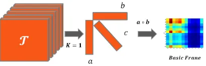
In the factorization stage, a tensorT is fed to the factorization procedure (Algorithm 3). This could be TN A or TIE depending on who calls the
fac-torization procedure. Using the CP facfac-torization, basic factors of the input tensor T are obtained (line 2). Using these basic factors the basic frame B
is computed (line 3). To obtain the basic frame, Equation 6 is used where
K = 1 and basic factors a and b represent previous and current heuristic indexes respectively (Figure 3). The values in the basic frame quantify the relationship between the elements along each dimension (basic factor). To make use of the basic frame, the maximum entry is pinpointed and the col-umn corresponding to this entry is sorted. This results in a vector S which contains the score values achieved for heuristics.
The factorization stage is applied to both TN A and TIE tensors. That is,
Fol-Algorithm 2: The tensor construction phase
1 In: h, acceptance criteria,P, tp;
2 Initialize tensor frameM to 0;
3 counter= 0; 4 while t < tp do
5 if counter=⌊|h|/2⌋ then
6 append Mto T;
7 set frame label to ∆f;
8 Initialize tensor frame M to 0;
9 counter = 0;
10 end
11 hprevious=hcurrent;
12 hcurrent = selectHeuristic(h);
13 fcurrent =fnew;
14 fnew =applyHeuristic(hcurrent); 15 δf =fcurrent−fnew;
16 if Accept(δf, acceptance criteria) then
17 mh
previous,hcurrent = 1;
18 mh
current,hprevious = 1;
19 counter+ +;
20 end
21 end
Figure 3: Extracting the basic frame forK= 1 in Eq.5.
lowing this, the two procedure (Algorithms 2 and 3) are executed assuming IE as acceptance criteria. This results in a basic frameBIE and score values
SIE. Consequently, for a given heuristic, there are two vectors of score values, one obtained from factorizing TN A and the other obtained from factorizing
TIE. These score vectors are sorted in line 5 and fed into the partitioning
procedure (Algorithm 4). Sorting of scores is necessary during the ranking of heuristics and partitioning the heuristic space in Algorithm 4.
Algorithm 3: Factorization
1 In: T,h;
2 a,b,c = CP(T, K = 1);
3 B=a◦b;
4 x, y =max(B);
5 S=sort(Bi=1:|h|,y) //Scores;
Algorithm 4 is used to partition the space of heuristics. In lines 2 and 3 of the algorithm, the two score values for a given heuristic are compared to one another. The heuristic is assigned to the set hN A if its score is higher (or equal) in the basic frame achieved from TN A (that is, if SN A(h)≥ SIE(h)).
Otherwise it is assigned to hIE. Note that, equal scores (say, SN A(h) =
SIE(h)) rarely happens. At the end of this procedure, two distinct sets of heuristics, hN A and hIE, are achieved where each group is associated to NA and IE acceptance methods respectively..
4.2. Parameter Control via Tensor Analysis
Algorithm 4: Partitioning
1 In: BN A,BIE,SN A,SIE;
2 hN A={h∈h | SN A(h)≥SIE(h)};
3 hIE ={h∈h | SIE(h)>SN A(h)};
0.5, 0.6, 0.7, 0.8}denoted by p∈P. The goal is to construct a tensor which contains selected heuristic parameter values per heuristic index. Factorizing this tensor would then help in associating each heuristic with a parameter value. This is while the final stage of the algorithm (Algorithm 6) runs for a longer time and uses these parameter values for each heuristic instead of choosing them randomly. Despite their similarity, each stage is described in detail here to provide the readers with a clearer picture of the logic
In Algorithm 5, the two sets of heuristics achieved in the previous stage together with their respective score values per heuristic are employed to run a hybrid acceptance hyper-heuristic. For the selected heuristic, a random parameter value is chosen and set (lines 11-12), the heuristic is applied and the relevant acceptance criteria is checked (lines 14-15). The heuristic se-lection is based on tournament sese-lection. Depending on the tour size, few heuristics are chosen from the heuristic set corresponding to the acceptance mechanism and a heuristic with highest score (probability) is chosen and ap-plied. In case of acceptance, the relevant frame entry is updated (line 16). Since this is a hybrid acceptance algorithm, each acceptance criteria has a budget which is expressed as the number of heuristic calls allocated to the acceptance method. If the acceptance criteria has used its budget, then a new random acceptance criteria is selected (lines 18-20). Obviously, in cases where there are only two acceptance methods available (like here) random selection can be replaced by simply toggling between the two acceptance methods. A random selection is however necessary for cases where there are more than two acceptance strategies available. After continuing this process for a time tp, the final tensor (TP aram) is constructed from collected frames
and factorized (exactly in the same manner as in Algorithm 2), the basic frame is computed and the parameter values are extracted as suggested in line 25.
4.3. Improvement Stage
Algorithm 5: Parameter Control
1 In: h,hN A,hIE,tp;
2 Initialize tensor frameM to 0;
3 counter= 0;
4 while t < tp do
5 if counter=⌊|h|/2⌋ then
6 append frame and initialize;
7 if acceptance criteria = NA then 8 h = SelectHeuristic(hN A);
9 else
10 h = SelectHeuristic(hIE); 11 pcurrent =rand({0.1,0.2,· · · ,0.8});
12 setHeuristicParameter(pcurrent);
13 fcurrent =fnew;
14 fnew =applyHeuristic(hcurrent) ,δf =fcurrent−fnew;
15 if Acceptance(δf, acceptance criteria) then
16 mh,p = 1 , counter+ +;
17 end
18 if callCounter > c then 19 callCounter = 0;
20 acceptance criteria = selectRandomAcceptance();
21 end
22 Construct final tensorTP aram from collected data; 23 a,b,c = CP(TP aram, K = 1);
24 B=a◦b;
25 x, y =max(B);
to run a hybrid acceptance hyper-heuristic (Algorithm 6). Each acceptance method is given a budget in terms of the maximum number of heuristic calls it is allowed to perform (callCounter). Whenever, the acceptance method uses its budget, the algorithm switches to a randomly chosen acceptance method, resetting the budget (line 10-12). Depending on the acceptance criteria in charge, a heuristic is selected (using the tournament selection method discussed above) from the corresponding set (lines 2-5). For instance, if NA is in charge a heuristic is selected from hN A. Later, depending on the nature of the heuristic (mutation, hill climbing or none) the parameter value of the heuristic is assigned (line 6) and the heuristic is applied (line 7). The achieved objective function value is then controlled for acceptance (line 9). This process continues until a time limit (3×tp) is reached.
Algorithm 6: Improvement
1 while t <(3×tp)do
2 if acceptance criteria = NA then
3 h = SelectHeuristic(hN A);
4 else
5 h = SelectHeuristic(hIE);
6 setHeuristicParameter(P(h));
7 fnew = ApplyHeuristic(h); 8 δf =fcurrent−fnew;
9 Acceptance(δf, acceptance criteria);
10 if callCounter > c then 11 callCounter = 0;
12 acceptance criteria = selectRandomAcceptance();
13 end
5.1. Experimental Design
The algorithm proposed here is a multi-stage algorithm where in each stage data samples are collected from the search process in form of tensors. Various approaches can be considered for data collection. While each stage can collect the data and ignore those collected in previous corresponding stages the data collected from various (corresponding) stages can be ap-pended to one another. The former data collection approach has the advan-tage that collected data reflect the current search status independent from previous search stages allowing the algorithm to focus on the current state. However, ignoring previous data means discarding the knowledge that could have been extracted from experience. In order to assess the two data collec-tion approaches, we employ both data colleccollec-tion approaches. That is, two methods are investigated here, both using the same algorithm (as in Algo-rithm 1). The only difference between them is that one algoAlgo-rithm (TeBHH 1) the data collection phase of the algorithm ignores previously collected data and over-writes the dataset. In the second algorithm (TeBHH 2) the data collected at each stage is appended to those collected in the same previous stage. Please note that, this does not mean that the data collected in the third stage is appended to those collected in the second stage. Each stage maintains its own dataset and e.g. stage 2 appends its data to the dataset designated for the same stage index.
5.2. Selecting The Best Performing Parameter Setting
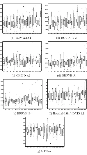
In order to determine the best performing parameter setting, each vari-ant of the algorithm with a parameter value combination was run 10 times where each run terminates after two hours. Apart from detecting the best performing parameter configuration, we would like to know how sensitive the framework is with respect to the parameter settings. Seven instances were chosen for these experiments which would hopefully cover and represent a whole range of available instances. The chosen instances are: BCV-A.12.1,
BCV-A.12.2, CHILD-A2, ERRVH-A, ERRVH-B, Ikegami-3Shift-DATA1.2 and
MER-A.
Figure 4 shows the results from these experiments for the TeBHH 1 vari-ant. Although most of the configurations seem to achieve similar perfor-mances, there is no other parameter configuration which performs signifi-cantly better than the configuration with index 9 (for which tp = 175 sec-onds, acceptance budget of 3× |h| and tournament size of 2) on any of the cases, which is confirmed via a Wilcoxon signed rank test. Ranking all con-figuration based on the average results across the instances shows that this configuration performs slightly better than the others in the overall. There-fore, these values are chosen for the TeBHH 1 variant. A similar analysis shows that the parameter configuration with index 4 (for which tp = 75 sec-onds, acceptance budget of 2× |h|and tournament size of 2) is more suitable for the TeBHH 2 variant. It has been observed that tournament size of 2 is constantly a winner over the other values for tour size. The apparent con-clusion is that both algorithms are very much sensitive to the value chosen for this parameter. Also, a shorter time for data collection in the TeBHH 2 variant makes sense, since it preserves the data collected in previous data collection sessions. The same is not true for TeBHH 1 which overwrites the old data in each stage. Thus, a longer data collection time in case of TeBHH 1 also makes sense. However, when the performance of variants with dif-ferent data collection time values are compared, the emerging conclusion is that both algorithms are not very sensitive to the chosen value. A similar conclusion can be reached for the value of the acceptance budget.
5.3. Comparative Study
1350 1400 1450 1500 1550 1600 1650
1 2 3 4 5 6 7 8 9 10 11 12 13 14 15 16 17 18 19 20 21 22 23 24 25 26 27
(a) BCV-A.12.1 1900 1950 2000 2050 2100 2150 2200
1 2 3 4 5 6 7 8 9 10 11 12 13 14 15 16 17 18 19 20 21 22 23 24 25 26 27
(b) BCV-A.12.2 1090 1095 1100 1105 1110 1115 1120 1125
1 2 3 4 5 6 7 8 9 10 11 12 13 14 15 16 17 18 19 20 21 22 23 24 25 26 27
(c) CHILD-A2 2140 2160 2180 2200 2220 2240
1 2 3 4 5 6 7 8 9 10 11 12 13 14 15 16 17 18 19 20 21 22 23 24 25 26 27
(d) ERRVH-A 3120 3140 3160 3180 3200 3220 3240
1 2 3 4 5 6 7 8 9 10 11 12 13 14 15 16 17 18 19 20 21 22 23 24 25 26 27
(e) ERRVH-B 8 10 12 14 16 18 20 22 24
1 2 3 4 5 6 7 8 9 10 11 12 13 14 15 16 17 18 19 20 21 22 23 24 25 26 27
(f) Ikegami-3Shift-DATA1.2 8900 9000 9100 9200 9300 9400 9500 9600
1 2 3 4 5 6 7 8 9 10 11 12 13 14 15 16 17 18 19 20 21 22 23 24 25 26 27
[image:26.595.155.454.164.699.2](g) MER-A
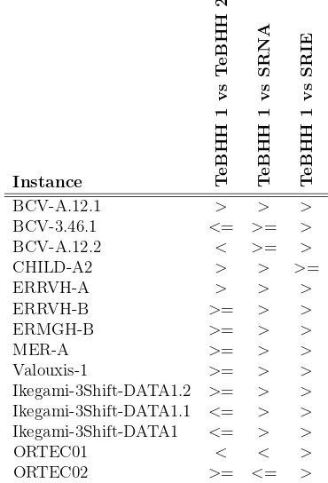
statistical test, based on Wilcoxon signed rank test, reveals that, the perfor-mance disparity between the two algorithms can vary from one instance to another. For instance, TeBHH 1 outperforms TeBHH 2 on 3 instances signif-icantly. This is while on 2 other instances the situation is the opposite. Also, on 9 instances there is no statistically significance difference between the per-formance of the two algorithms. This makes sense since the only difference between the two algorithms is the way the dataset is treated throughout the time. While TeBHH 1 overwrites the data with newly collected dataset, TeBHH 2 appends the new data to the old dataset. Thus, it is natural that TeBHH 2 performs similarly to TeBHH 1 since much of their collected data can be similar. Also, the heuristics on all nurse rostering instances are quite slow and therefore there is a lack of data which is more the reason that the two algorithms perform similarly.
Overall, combining the entries in Table 2 and the minimum objective function value achieved by each algorithm (Table 3), it would be fair to say that TeBHH 1 performs slightly better than TeBHH 2. It is to say that it would be safer to refresh the dataset once in a while and handle the current search landscape independent from the experience achieved from other regions of the search landscape.
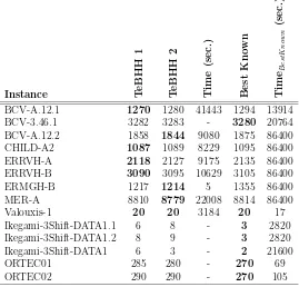
Subsequent to this conclusion another statistical experiment is conducted to compare the performance of the TeBHH 1 to its building block compo-nents, namely, SR-NA and SR-IE. The third and fourth columns in Table 2 shows that, given equal values as run time, TeBHH1 performs always better than the SR-IE hyper-heuristic. On only one instance, TeBHH 1 performs slightly (and not significantly) better. As for the comparison between TeBHH 1 and NA, although TeBHH 1 still performs significantly better than SR-NA on the majority of instances, onORTECinstances it performs very poorly. The results of applying the two proposed algorithms on various nurse rostering instances is shown in Table 3. The two algorithms are also com-pared to various well-known algorithms. While some of these algorithms (like the one in (Chan et al., 2012)) are general-purpose search algorithms, some others are specifically designed to solve the given instance.
Instance Te
B
H
H
1
v
s
T
e
B
H
H
2
T
e
B
H
H
1
v
s
S
R
N
A
T
e
B
H
H
1
v
s
S
R
IE
BCV-A.12.1 > > >
BCV-3.46.1 <= >= >
BCV-A.12.2 < >= >
CHILD-A2 > > >= ERRVH-A > > >
ERRVH-B >= > >
ERMGH-B >= > >
MER-A >= > >
Valouxis-1 >= > >
Ikegami-3Shift-DATA1.2 >= > >
Ikegami-3Shift-DATA1.1 <= > >
Ikegami-3Shift-DATA1 <= > >
ORTEC01 < < >
[image:28.595.213.398.268.540.2]ORTEC02 >= <= >
Instance Te B H H 1 T e B H H 2 T im e (s e c .) B e st K n o w n T im eB e s tK n o w n (s e c .)
[image:29.595.173.442.178.436.2]BCV-A.12.1 1270 1280 41443 1294 13914 BCV-3.46.1 3282 3283 - 3280 20764 BCV-A.12.2 1858 1844 9080 1875 86400 CHILD-A2 1087 1089 8229 1095 86400 ERRVH-A 2118 2127 9175 2135 86400 ERRVH-B 3090 3095 10629 3105 86400 ERMGH-B 1217 1214 5 1355 86400 MER-A 8810 8779 22008 8814 86400 Valouxis-1 20 20 3184 20 17 Ikegami-3Shift-DATA1.1 6 8 - 3 2820 Ikegami-3Shift-DATA1.2 8 9 - 3 2820 Ikegami-3Shift-DATA1 6 3 - 2 21600 ORTEC01 285 280 - 270 69 ORTEC02 290 290 - 270 105
Table 3: Comparison between the two proposed algorithms and various well-known (hyper-/meta-)heuristics. The second and third columns contain the best objective function values achieved by TeBHH 1 and TeBHH 2 respectively. Fourth column gives the earliest CPU time (seconds) in which the reported result in bold has been achieved by the corresponding proposed algorithm. ‘-’ denotes that the maximum CPU time has been used up without improving upon the best known result. Same quantities (minimum objective function values and earliest time it has been achieved) are also reported for compared algorithms in columns five and six.
instances are instance-specific and designed to solve a group of highly related instances, such as those in the Ikegami family. Overall, the two algorithms perform well on provided instances and produce new best known results for some of them (the first seven instances).
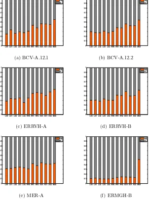
Figure 5 shows the distribution of heuristics to disjoint setshN A and hIE
from one instance to another. The difference between histograms are some-times minor (as it is between histograms of BCV-A.12.1 and BCV-A.12.2) and sometimes major (as is the case for the instance MER-A compared to the rest). However, the common pattern among most of these partitions is that the heuristic MU0 has been equally associated to both sets. Although the framework clearly shows the tendency to assign heuristics more to the hIE
set rather than hN A, Ruin Recreate and Crossover heuristics are likelier to be assigned to hN A compared to local search heuristics. Since the heuristics in nurse rostering domain all deliver feasible solutions, it makes sense that the framework tries to increase the possibility of diversification by assigning diversifying heuristics to NA acceptance method.
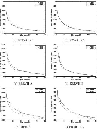
During the improvement stage (Algorithm 6), the algorithm allocates a time budget to each acceptance method. Whenever this budget is consumed, the algorithm switches to a randomly chosen acceptance criteria. Since the tensor analysis is likelier to assign diversifying heuristics tohN A(keeping the intensifying heuristics inhIE), it thus performs similar to a higher level Iter-ated Local Search (ILS) algorithm where each intensification step is followed by a diversification one. That in turn results in continuous improvement of the solution as is confirmed in Figure 6 for TeBHH 1 and TeBHH 2 respec-tively.
The progress plots corresponding to TeBHH 1 and TeBHH 2 (Figure 6) show that on many instances (particularly on BCV-A.12.1, BCV-A.12.2 and
ERMGH-B) both algorithm are rarely stuck in local optima. This is a good
behaviour showing that given longer run times (similar to the experiments in (Chan et al., 2012)) there is a high likelihood that the algorithms proposed here provide better results with even lower objective function values.
6. Conclusions
LS0 LS1 LS2 LS3 LS4 RR0 RR1 RR2 XO0 XO1 XO2 MU0 0 0.1 0.2 0.3 0.4 0.5 0.6 0.7 0.8 0.9 1 NA IE (a) BCV-A.12.1
LS0 LS1 LS2 LS3 LS4 RR0 RR1 RR2 XO0 XO1 XO2 MU0 0 0.1 0.2 0.3 0.4 0.5 0.6 0.7 0.8 0.9 1 NA IE (b) BCV-A.12.2
LS0 LS1 LS2 LS3 LS4 RR0 RR1 RR2 XO0 XO1 XO2 MU0 0 0.1 0.2 0.3 0.4 0.5 0.6 0.7 0.8 0.9 1 NA IE (c) ERRVH-A
LS0 LS1 LS2 LS3 LS4 RR0 RR1 RR2 XO0 XO1 XO2 MU0 0 0.1 0.2 0.3 0.4 0.5 0.6 0.7 0.8 0.9 1 NA IE (d) ERRVH-B
LS0 LS1 LS2 LS3 LS4 RR0 RR1 RR2 XO0 XO1 XO2 MU0 0 0.1 0.2 0.3 0.4 0.5 0.6 0.7 0.8 0.9 1 NA IE (e) MER-A
[image:31.595.156.460.235.644.2]LS0 LS1 LS2 LS3 LS4 RR0 RR1 RR2 XO0 XO1 XO2 MU0 0 0.1 0.2 0.3 0.4 0.5 0.6 0.7 0.8 0.9 1 NA IE (f) ERMGH-B
0 100 200 300 400 500 1350 1400 1450 1500 1550 1600 1650 1700 time (minutes)
objective function value
TeBHH 1 TeBHH 2
(a) BCV-A.12.1
0 100 200 300 400 500
1900 1950 2000 2050 2100 2150 2200 2250 time (minutes)
objective function value
TeBHH 1 TeBHH 2
(b) BCV-A.12.2
0 100 200 300 400 500
2140 2150 2160 2170 2180 2190 2200 2210 2220 time (minutes)
objective function value
TeBHH 1 TeBHH 2
(c) ERRVH-A
0 100 200 300 400 500
3120 3130 3140 3150 3160 3170 3180 3190 3200 3210 time (minutes)
objective function value
TeBHH 1 TeBHH 2
(d) ERRVH-B
0 100 200 300 400 500
9000 9100 9200 9300 9400 9500 9600 9700 time (minutes)
objective function value
TeBHH 1 TeBHH 2
(e) MER-A
0 100 200 300 400 500
1280 1290 1300 1310 1320 1330 1340 1350 1360 time (minutes)
objective function value
TeBHH 1 TeBHH 2
[image:32.595.143.467.210.640.2](f) ERMGH-B
that ‘forgetting’ is slightly more useful than remembering all. Hence, a strat-egy that decides on the memory length adaptively would be of interest as a future work. In this study, the tensor-based hyper-heuristic with memory refresh generated new best solutions for four benchmark instances and a tie on one of the benchmark instance.
The proposed approach cycles through four stages continuously and peri-odically, employing machine learning in the first three stages to configure the algorithm to be used in the final stage. The final stage approach itself is an iterated multi-stage algorithm, invoking a randomly chosen hyper-heuristic at each stage. Depending on the problem instance and even a trial, the nature of the low level heuristics allocated to each stage (hence the move acceptance) could change. However, experiments indicate that mutational heuristics often can get allocated to either of the hyper-heuristics. SR-NA allows worsening moves while SR-IE does not. Hence, the final stage compo-nent of the tensor-based hyper-heuristic acts as a high level Iterated Local Search algorithm (Louren¸co et al., 2010), providing a neat balance between intensification and diversification using the appropriate low level heuristics which are determined automatically during the search process, resulting in continuous improvement in time. The overall approach is enabled to extract fresh knowledge periodically throughout the run time, which is an extremely desired behavior in life-long learning. Thus, the tensor-based hyper-heuristic proposed here can be considered in life-long learning applications.
References
Acar, E., Dunlavy, D., Kolda, T., Dec 2009. Link prediction on evolving data using matrix and tensor factorizations. In: IEEE International Conference on Data Mining Workshops, 2009. ICDMW ’09. pp. 262–269.
Anandkumar, A., Ge, R., Hsu, D., Kakade, S. M., Telgarsky, M., 2012. Tensor decompositions for learning latent variable models. CoRR abs/1210.7559.
Anwar, K., Awadallah, M., Khader, A., Al-betar, M., 2014. Hyper-heuristic approach for solving nurse rostering problem. In: Computational Intelli-gence in Ensemble Learning (CIEL), 2014 IEEE Symposium on. pp. 1–6.
Asta, S., ¨Ozcan, E., 2015. A tensor-based selection hyper-heuristic for cross-domain heuristic search. Information Sciences 299 (0), 412 – 432.
URLhttp://www.sciencedirect.com/science/article/pii/S0020025514011591
Asta, S., ¨Ozcan, E., Parkes, A. J., Etaner-Uyar, A. c., 2013. Generalizing hyper-heuristics via apprenticeship learning. In: Proceedings of the 13th European Conference on Evolutionary Computation in Combinatorial Op-timization. EvoCOP’13. Springer-Verlag, Berlin, Heidelberg, pp. 169–178.
Azaiez, M. N., Al Sharif, S. S., Mar. 2005. A 0-1 goal programming model for nurse scheduling. Comput. Oper. Res. 32 (3), 491–507.
Bilgin, B., ¨Ozcan, E., Korkmaz, E., 2007. An experimental study on hyper-heuristics and exam timetabling. In: Burke, E., Rudov´a, H. (Eds.), Prac-tice and Theory of Automated Timetabling VI. Vol. 3867 of Lecture Notes in Computer Science. Springer Berlin Heidelberg, pp. 394–412.
URL http://dx.doi.org/10.1007/978-3-540-77345-0_25
Brucker, P., Burke, E., Curtois, T., Qu, R., Vanden Berghe, G., 2010. A shift sequence based approach for nurse scheduling and a new benchmark dataset. Journal of Heuristics 16 (4), 559–573.
Burke, E., Curtois, T., Hyde, M., Kendall, G., Ochoa, G., Petrovic, S., V´azquez-Rodr´ıguez, J., Gendreau, M., July 2010a. Iterated local search vs. hyper-heuristics: Towards general-purpose search algorithms. In: 2010 IEEE Congress on Evolutionary Computation (CEC). pp. 1–8.
Burke, E. K., Curtois, T., 2014. New approaches to nurse rostering bench-mark instances. European Journal of Operational Research 237 (1), 71–81.
Burke, E. K., Curtois, T., Post, G., Qu, R., Veltman, B., 2008. A hybrid heuristic ordering and variable neighbourhood search for the nurse rostering problem. European Journal of Operational Research 188 (2), 330–341.
URLhttp://www.sciencedirect.com/science/article/pii/S0377221707004390
Burke, E. K., De Causmaecker, P., Berghe, G. V., Van Landeghem, H., Nov. 2004. The state of the art of nurse rostering. J. of Scheduling 7 (6), 441– 499.
Burke, E. K., Gendreau, M., Hyde, M., Kendall, G., Ochoa, G., ¨Ozcan, E., Qu, R., 2013. Hyper-heuristics: A survey of the state of the art. Journal of the Operational Research Society 64 (12), 1695–1724.
Burke, E. K., Hyde, M., Kendall, G., Ochoa, G., ¨Ozcan, E., Woodward, J. R., 2010c. A classification of hyper-heuristics approaches. In: Gendreau, M., Potvin, J.-Y. (Eds.), Handbook of Metaheuristics, 2nd Edition. Vol. 57 of International Series in Operations Research & Management Science. Springer, Ch. 15, pp. 449–468.
Burke, E. K., Kendall, G., Soubeiga, E., 2003. A tabu-search hyperheuristic for timetabling and rostering. Journal of Heuristics 9 (6), 451–470.
Burke, E. K., Li, J., Qu, R., 2010d. A hybrid model of integer programming and variable neighbourhood search for highly-constrained nurse rostering problems. European Journal of Operational Research 203 (2), 484 – 493.
Carroll, J., Chang, J.-J., 1970. Analysis of individual differences in multidi-mensional scaling via an n-way generalization of eckart-young decomposi-tion. Psychometrika 35 (3), 283–319.
Chan, C., Xue, F., Ip, W., Cheung, C., 2012. A hyper-heuristic inspired by pearl hunting. In: Hamadi, Y., Schoenauer, M. (Eds.), Learning and Intel-ligent Optimization. Lecture Notes in Computer Science. Springer Berlin Heidelberg, pp. 349–353.
URL http://dx.doi.org/10.1007/978-3-642-34413-8_26
Cichocki, A., Mandic, D. P., Phan, A. H., Caiafa, C. F., Zhou, G., Zhao, Q., Lathauwer, L. D., 2014. Tensor decompositions for signal process-ing applications from two-way to multiway component analysis. CoRR abs/1403.4462.
URL http://arxiv.org/abs/1403.4462
Curtois, T., 2015. Published results on employee scheduling instances.
http://www.cs.nott.ac.uk/~tec/NRP/.
Curtois, T., Ochoa, G., Hyde, M., V´azquez-Rodr´ıguez, J. A., 2009. A hyflex module for the personnel scheduling problem. Tech. rep., School of Com-puter Science, University of Nottingham.
Glass, C. A., Knight, R. A., 2010. The nurse rostering problem: A criti-cal appraisal of the problem structure. European Journal of Operational Research 202 (2), 379 – 389.
Harshman, R. A., 1976. PARAFAC: Methods of three-way factor analysis and multidimensional scaling according to the principle of proportional profiles. Ph.D. thesis, University of California, Los Angeles, CA.
Hart, E., Sim, K., 2014. On the life-long learning capabilities of a nelli*: A hyper-heuristic optimisation system. In: Bartz-Beielstein, T., Branke, J., Filipi, B., Smith, J. (Eds.), Parallel Problem Solving from Nature PPSN XIII. Vol. 8672 of Lecture Notes in Computer Science. Springer Interna-tional Publishing, pp. 282–291.
URL http://dx.doi.org/10.1007/978-3-319-10762-2_28
Haspeslagh, S., De Causmaecker, P., Schaerf, A., Stlevik, M., 2014. The first international nurse rostering competition 2010. Annals of Operations Research 218 (1), 221–236.
URL http://dx.doi.org/10.1007/s10479-012-1062-0
Karp, R., 1972. Reducibility among combinatorial problems. In: Miller, R., Thatcher, J., Bohlinger, J. (Eds.), Complexity of Computer Computations. The IBM Research Symposia Series. Springer US, pp. 85–103.
URL http://dx.doi.org/10.1007/978-1-4684-2001-2_9
Kim, T.-K., Cipolla, R., Aug. 2009. Canonical correlation analysis of video volume tensors for action categorization and detection. IEEE Trans. Pat-tern Anal. Mach. Intell. 31 (8), 1415–1428.
Kolda, T. G., Bader, B. W., Aug. 2009. Tensor decompositions and applica-tions. SIAM Rev. 51 (3), 455–500.
Lathauwer, L. D., Moor, B. D., Vandewalle, J., Mar. 2000. A multilinear singular value decomposition. SIAM J. Matrix Anal. Appl. 21 (4), 1253– 1278.
Loudni, S., Boizumault, P., 2008. Combining vns with constraint program-ming for solving anytime optimization problems. European Journal of Op-erational Research 191 (3), 705 – 735.
Louren¸co, H. R., Martin, O. C., St¨utzle, T., 2010. Iterated local search: Framework and applications. In: Gendreau, M., Potvin, J.-Y. (Eds.), Handbook of Metaheuristics. Vol. 146 of International Series in Opera-tions Research & Management Science. Springer US, pp. 363–397.
L¨u, Z., Hao, J.-K., 2012. Adaptive neighborhood search for nurse rostering. European Journal of Operational Research 218 (3), 865 – 876.
URLhttp://www.sciencedirect.com/science/article/pii/S0377221711010939
M´etivier, J.-P., Boizumault, P., Loudni, S., 2009. Solving nurse rostering problems using soft global constraints. In: Gent, I. (Ed.), Principles and Practice of Constraint Programming - CP 2009. Vol. 5732 of Lecture Notes in Computer Science. Springer Berlin Heidelberg, pp. 73–87.
Nareyek, A., 2004. Choosing search heuristics by non-stationary reinforce-ment learning. In: Resende, M. G. C., de Sousa, J. P., Viana, A. (Eds.), Metaheuristics. Kluwer Academic Publishers, Norwell, MA, USA, pp. 523– 544.
URL http://dl.acm.org/citation.cfm?id=982409.982435
Ochoa, G., Hyde, M., Curtois, T., Vazquez-Rodriguez, J., Walker, J., Gen-dreau, M., Kendall, G., McCollum, B., Parkes, A., Petrovic, S., Burke, E., 2012. Hyflex: A benchmark framework for cross-domain heuristic search. In: Hao, J.-K., Middendorf, M. (Eds.), European Conference on Evolu-tionary Computation in Combinatorial Optimisation, EvoCOP ’12. Vol. 7245 of LNCS. Springer, Heidelberg, pp. 136–147.
Pillay, N., Rae, C., 2012. A survey of hyper-heuristics for the nurse roster-ing problem. In: Proceedroster-ings of the 2012 ORSSA (Operations Research Society of South Africa) Annual Conference. pp. 115–122.
10th International Conference on the Practice and Theory of Automated Timetabling. pp. 527–532.
Shashua, A., Hazan, T., 2005. Non-negative tensor factorization with appli-cations to statistics and computer vision. In: ICML. pp. 792–799.
Silver, D., Yang, Q., Li, L., 2013. Lifelong machine learning systems: Beyond learning algorithms. In: AAAI Spring Symposium Series. pp. 49–55.
URLhttps://www.aaai.org/ocs/index.php/SSS/SSS13/paper/view/5802/5977
Sim, K., Hart, E., 2014. An improved immune inspired hyper-heuristic for combinatorial optimisation problems. In: Proceedings of the 2014 Confer-ence on Genetic and Evolutionary Computation. GECCO ’14. ACM, New York, NY, USA, pp. 121–128.
URL http://doi.acm.org/10.1145/2576768.2598241
Solos, I. P., Tassopoulos, I. X., Beligiannis, G. N., 2013. A generic two-phase stochastic variable neighborhood approach for effectively solving the nurse rostering problem. Algorithms 6 (2), 278–308.
Tucker, L. R., 1966c. Some mathematical notes on three-mode factor analysis. Psychometrika 31, 279–311.
Valouxis, C., Gogos, C., Goulas, G., Alefragis, P., Housos, E., 2012. A systematic two phase approach for the nurse rostering problem. European Journal of Operational Research 219 (2), 425 – 433.
URLhttp://www.sciencedirect.com/science/article/pii/S0377221711011362
Vasilescu, M. A. O., Terzopoulos, D., 2002. Multilinear analysis of image ensembles: Tensorfaces. In: Heyden, A., Sparr, G., Nielsen, M., Johansen, P. (Eds.), ECCV (1). Vol. 2350 of Lecture Notes in Computer Science. Springer, pp. 447–460.
Wang, D., Zhou, J., He, K., Liu, C., Xia, J., Oct 2009. Using tucker de-composition to compress color images. In: 2nd International Congress on Image and Signal Processing, 2009. CISP ’09. pp. 1–5.
Zou, B., Li, C., Tan, L., Chen, H., 2015. Gputensor: Efficient tensor factorization for context-aware recommendations. Information Sciences 299 (0), 159 – 177.