Abstract — Information on the best probability models in
representing the weekly distribution of dry and wet spells is increasingly important in various sectors including hydrological and water resource management. The application of the mixed probability models such as the mixture among the log series and geometric, Poisson as well as the truncated distributions is considered in fitting the observed data sets. In addition, the success of the higher order Markov chain models up to the tenth order is also compared with the mixed probability models. The performance of the best fitted models is assessed by using the Kolmogorov-Smirnov goodness-of-fit test in twelve selected rainfall stations from 1975 to 2010. The findings indicate that the mixture log series and truncated Poisson (MLTPD) are found to successfully fit the observed distribution of the weekly dry spells, while, the mixture log series and truncated geometric distribution (MGTPD) are more appropriate for the wet spells. The results obtained from the best fitted probability models will be used to produce the weekly dry and wet spells indices such as the mean and the maximum length of spells as well as the frequency of short and long spells.
Index Terms — Dry wet spells, Kolmogorov-Smirnov
goodness-of-fit test, Markov chain models, mixed probability models
I. INTRODUCTION
UE to the rapid growth of the Malaysian population and the development of industrialization, the management of water resources is increasingly in demand. Thus, relevant and useful information of daily, weekly or monthly rainfall analyses could be provided to ensure that the water system management works efficiently. Identification of the most appropriate probability models in representing the sequence of dry (wet) events is becoming important to the hydrological, agricultural and other water related sectors. The results of the best fitting models obtained could be used for data generation and prediction purposes.
The application of the various types of probability models in representing the distribution of the dry and wet spells was
Manuscript received Mar 01, 2012; revised Mar 12, 2012. This work was supported in part by the Malaysian Fundamental Research Grant, 600-RMI/ST/FRGS 5/3/FST (192/2010).
S. M. Deni. Center for Statistical and Decision Science Studies, Faculty of Computer and Mathematical Sciences, UiTM Shah Alam, 40450 Shah Alam, Selangor, Malaysia.(corresponding author: phone: +603-5543-5455; fax: +603-5543-5503; e-mail: sayang@ tmsk.uitm.edu.my).
A. A. Jemain. Center for Mathematical Sciences, Faculty of Science and Technology, 43600 UKM, Bangi, Selangor, Malaysia (e-mail: [email protected]).
started by previous researchers since the early part of the 20th century [1]-[4]. The mixture distributions such as the mixed two geometric distributions and the mixed geometric with Poisson distribution were also introduced by previous researchers [5]-[6].
The development of the probability models has continuously been explored by introducing five types of new mixed probability models such as mixed two log series (MLSD), mixed log series and geometric (MLGD), mixed log series and Poisson (MLPD), mixed log series and truncated Poisson distribution (MLTPD), and mixed log series and truncated geometric distribution (MGTPD) [7]. The recent study indicated that the MLTPD was proven to be the most frequent best model selected in representing the observed distribution of both the annual dry and wet spells in most of the stations in Peninsular Malaysia [8]. Alternatively, the application of the Markov chain models in describing the distribution of the dry and wet spells has been carried out by a number of researchers at various locations [9]-[17].
Most of the studies on rainfall distribution over Peninsular Malaysia are conducted based on daily and monthly rainfall data. The study on a weekly basis to determine the best model for the distribution of dry and wet spells has been successfully conducted in Sabah and Sarawak as reported in [18]. To date, the study on weekly dry and wet spells over the peninsula has yet to be conducted. The analysis of the different levels such as for the hourly, daily, monthly and also weekly basis cannot be neglected since it could provide valuable information for various applications including agricultural planning and management, as well as preventing the outbreak of waterborne diseases, designing the drainage and irrigation systems and predicting the dry and wet spells phenomena.
Although a lot of work on the identification of the best order of the Markov chain models as well as fitting the mixture probability models has been done on rainfall data from various parts of the world including Malaysia, however, little attention has been given to research on considering the weekly distribution of the wet and dry spells by comparing both types of the models together. Hence, this study is aimed to identify the best fitting models among the mixture distributions and Markov chain models for twelve selected rainfall stations in Peninsular Malaysia during the monsoonal seasons and as an annual basis. The weekly distribution of the wet and dry spells obtained from the results of the best fitted models will be used to produce the wet and dry indices such as the mean, maximum spells, and the frequency of short and long spells.
Comparison between Mixed Probability Models
and Markov Chain Models for Weekly Dry and
Wet Spells in Peninsular Malaysia
Sayang Mohd Deni and Abdul Aziz Jemain
II. DATAANDMETHODS
A. Data and the study area
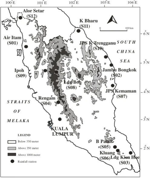
Peninsular Malaysia lies entirely in the equatorial zone which is situated in the northern latitude between 1o and 6o Nand in the eastern longitude from 100o to 103oE. There are two types of monsoons that influence the climate of the country, namely the Southwest monsoon (May to August) and the Northeast monsoon (November to February). The data used in this study are collected from the database of the Malaysian Meteorological Department (MMD) and the Drainage and Irrigation Department (DID), for the period of records that ranged from 1975 to 2010. The analysis of this study will be carried out based on the annual basis (ANNL) as well as the two types of monsoons and the inter monsoon periods i.e. the first inter monsoon with the Southwest monsoon (FISW) and the second inter monsoon with the Northeast monsoon (SINE). Figure 1 shows the location of the 12 selected rainfall stations in Peninsular Malaysia. Moreover, the homogeneity of the data series are checked using three out of the four types of homogeneity tests such as the standard normal homogeneity test (SHNT), the Buishand range test (BRT) and the Von Neumann (VonNR) ratio test as recommended by [19]-[20]. The missing values in the data series for the periods of 1975 to 2010 are estimated using various types of weighting methods such as the inverse distance, the normal ratio and the correlation between the target and the neighboring stations [20]–[24]. A wet or dry spell can be defined as a prolonged period of wet or dry weather respectively. A week of rainfall amount with less than the threshold value will be classified as dry week and vice versa, a week of rainfall amounting to more than the threshold value is defined as a wet week. In this study, the weekly rainfall data are derived from the accumulated five days of daily rainfall data with a total
rainfall amount of at least 5.0 mm. Otherwise, the week is considered as a dry week.
B. Mixed probability models
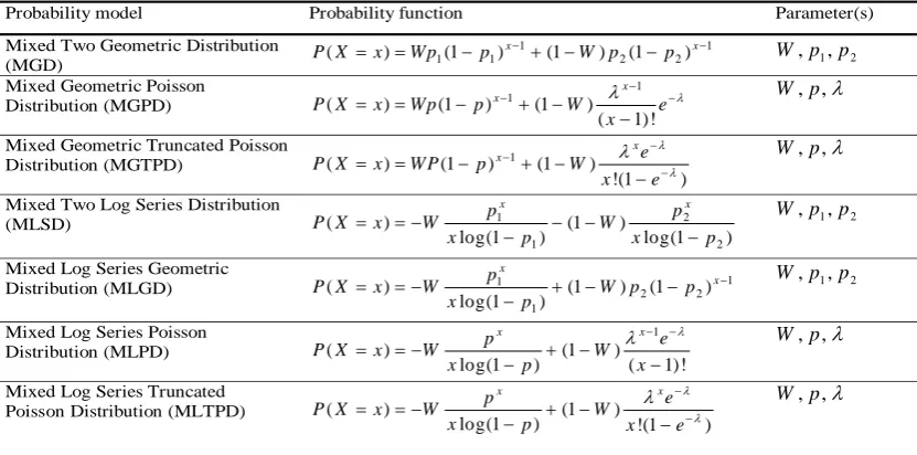
The mixed probability models i.e. MGD, MGPD, MLSD, MLGD, MGTPD, MLPD and MLTPD which were introduced by previous researchers [5]-[7] will be applied to the weekly distribution of dry and wet spells at each of the 12 rainfall stations in Peninsular Malaysia. The mixed probability models with their probability functions as well as the parameter(s) are displayed in Table 1. The parameters of the probability models are estimated using the maximum likelihood method. The maximum likelihood estimates are computed by implementing the R or S-Plus function for optimization under the quasi-Newton procedure [25]. The parameter ofp p, 1and p2 for each mixed probability model applied ranges from 0 to 1, while W is the weight factor, where the sum of W and (1W) is unity.
C. Markov chain models
Let X X1, 2,,Xt,,Xn denote n binary variables to represent the sequences of wet and dry events in the weekly rainfall occurrence for n–arbitrary weeks, indicated as 1 and 0, respectively. A wet (dry) spell is defined as a period of consecutive weeks of exactly, say n wet (dry) weeks, occurring exactly before a dry (wet) week and returning to the wet (dry) condition in the (n1)thweek. The first order Markov chain only takes into account the condition of the state, either wet or dry, for one preceding week. Similarly, the second order considers the states of the two preceding weeks and so on. The Markov chain models up to order ten are applied in this present study. The joint probabilities of the kth order of the Markov chain models are defined as follows:
21 1 1
2 1 , ,
[image:2.595.43.291.476.770.2]1
( , , | ) , 1; 0,1
k k j j
n k
n i i i i i i
j
Pi i i P P P n k k
(1)
The conditional probability of two consecutive wet weeks can be written asP(011| 0). The rest of the consecutive wet weeks will follow the same rule, i.e. three consecutive weeks is denoted as P(0111|0) and so forth. In order to compute the expected number of wet weeks, the conditional probabilities according to the respective length, say, 1, 2, 3, …, n weeks, which is obtained from Eq. (1) will be multiplied by the total number of dry weeks.
A. Model selection
The Kolmogorov-Smirnov goodness-of-fit test will be employed to compare the observed distribution and the expected distributions of the dry and wet spells which are obtained from the mixed probability models as well as the Markov chain models. The maximum absolute difference,
Dmax, between the two cumulative values of the observed
and expected number of dry and wet days under the assumed models are computed and if these values are found to be less than or equal to the critical value
D
0.05, the particular models are considered as best to describe the distribution of the weekly dry and wet spells. Alternatively, the Akaike’s Information Criteria could be considered in selecting the best mixed models as suggested by previous researchers [7-8], [17].0 10 0 km
LEGEND Below 350 meter Above 350 meter
Above 1000 meter
Rainfall station
S T R A I T S
O F
M E L A K A
S O U T H C H I N A
S E A
100 E 101 E 102 E 103 E
O O O O
104 E
O
6 N
O
5 N
O
4 N
3 N
2 N
O
O
O JPS Kemaman (S07)
Kluang (S06)
Jambu Bongkok (S02) Air Itam
(S01)
Rengam (S04)
Ldg Kien Hoe (S03) B Pahat (S05) JPS K Trengganu (S10) K Bharu (S11)
Ipoh (S09)
Ldg Boh (S08) Alor Setar
(S12)
.
KUALA LUMPUR
TABLE 1
The probability models, their probability functions and the parameter(s) used for fitting the distribution of weekly dry and wet spells. For each of the following probability functions, x1, 2,.
III. RESULTSANDDISCUSSION
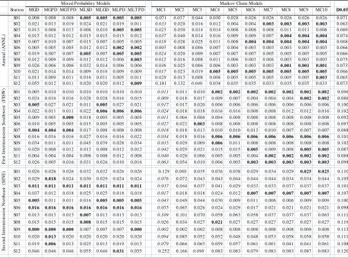
The selected probability models as shown in Table 2 and 3 (in bold face) were based on a best fit of the Kolmogorov-Smirnov GOF test in describing the weekly distribution of the dry or wet spells to a particular probability model at the 5% level of significance. The results in Table 2 revealed that more than one model was found to best fit at a particular station. For example the analysis of the annual basis indicated that there were four mixed probability models i.e. MLSD, MLGD, MLPD and MLTPD found to best fit the distribution of the weekly dry spells at Station S01. Since the number of estimated parameters was the same for each of the mixed probability models, either one of these four models could be chosen to represent the respective data set. However, for the Markov chain models, the higher order model required the larger number of parameters. As indicated in Table 2, the findings showed that the Markov chain models of the seventh up to the tenth order were found to best fit the distribution of the weekly dry spells at station S02. In this case, the MC7 was chosen instead of the MC8 to MC10, due to the lesser numbers of parameters required.
Generally, in selecting the best probability models, the model with the least number of parameters is preferred. In this study, the three parameter models i.e. MLTPD and MGTPD were preferably selected in representing the weekly dry and wet spells respectively compared to the higher order Markov chain models i.e. MC2 to MC10. Moreover, these models were chosen due to their ability to successfully best fit most of the selected twelve stations in Peninsular Malaysia during the ANNL as well as in both seasons. The results of the Markov chain models which significantly fitted the observed data as indicated in Tables 2 and 3 (in italic face), revealed that most of the weekly dry spells could be described by the first order of the Markov chain models, except at Stations S01 and S12 during the ANNL and SINE
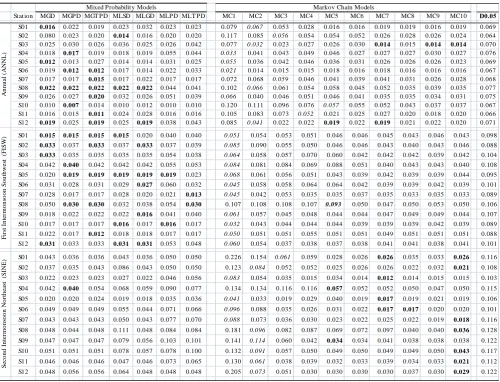
periods. For the weekly wet spells during ANNL as indicated in Table 3, seven out of the twelve stations were found to significantly fit the higher order Markov chain models. The results indicated that the fifth order of the Markov chain models (MC5) significantly fitted the weekly distribution of the wet spells at Station S10. In this situation, it was more appropriate to consider the mixed probability models rather than the Markov chain models in identifying the best fit models at this station (S10).
Moreover, Figure 2 displays the observed and the expected distributions of the weekly dry spells during the ANNL at Station S01 obtained from the selected probability models MLTPD and MC7. It could be seen that the expected frequency of the dry spells which were obtained from these models actually described the observed distribution. With the application of each probability model to the data sets, further analysis will identify the weekly indices of the dry and wet spells such as the mean and the maximum length of spells as well as the frequency of short (1-2 weeks) and long (more than 2 weeks) spells selected at each of the rainfall station in Peninsular Malaysia. This information will benefit the hydrologist, agriculturist and the water resource management in predicting future climatic events.
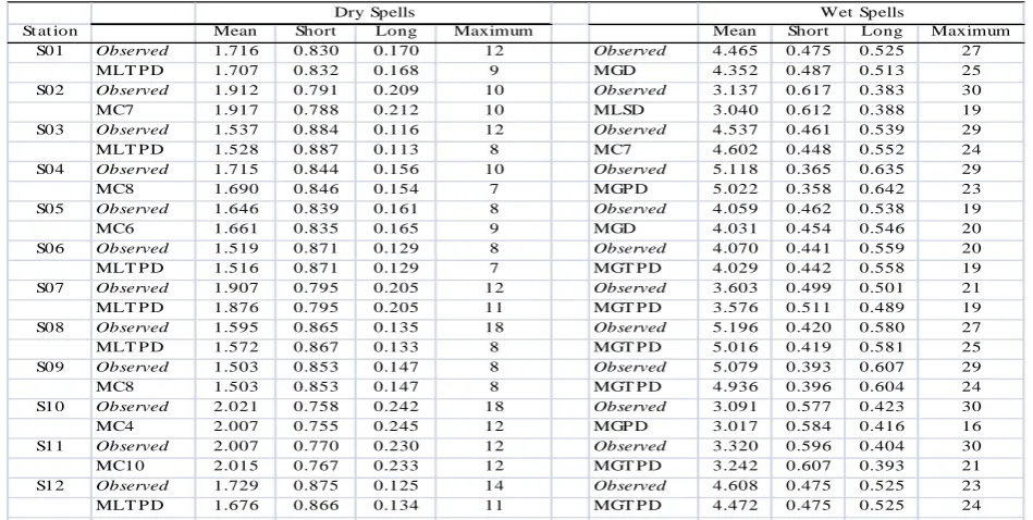
The indices of the wet and dry spells of the weekly observed and expected frequency distributions of the best fitted probability model at each station for dry and wet spells conducted on the annual basis are shown in Table 4. The indices found for the theoretical distribution which included the mean, maximum length of weekly dry (wet) spells, proportion of short spells (1-2 weeks), and long spells (more than 2 weeks) of the expected frequency of dry (wet) spells for the best probability models selected at each of the rainfall stations could reasonably be used to describe the underlying observed weekly distribution of dry (wet) spells. For example, it has been demonstrated in Figure 2 that the best probability model identified at station S02 was found to
Probability model Probability function Parameter(s)
Mixed Two Geometric Distribution (MGD)
1 1
1 1 2 2
( ) (1 )x (1 ) (1 )x
P X x W p p W p p W p, 1,p2
Mixed Geometric Poisson Distribution (MGPD)
1 1
( ) (1 ) (1 )
( 1)!
x x
P X x Wp p W e
x
, ,
W p
Mixed Geometric Truncated Poisson
Distribution (MGTPD) ( ) (1 ) 1 (1 )
!(1 )
x
x e
P X x W P p W
x e
, ,
W p
Mixed Two Log Series Distribution
(MLSD) 1 2
1 2
( ) (1 )
log(1 ) log(1 )
x x
p p
P X x W W
x p x p
1 2
, ,
W p p
Mixed Log Series Geometric
Distribution (MLGD) 1 2 2 1
1
( ) (1 ) (1 )
log(1 )
x
x
p
P X x W W p p
x p
1 2
, ,
W p p
Mixed Log Series Poisson Distribution (MLPD)
1
( ) (1 )
log(1 ) ( 1)!
x x
p e
P X x W W
x p x
, ,
W p
Mixed Log Series Truncated
Poisson Distribution (MLTPD) ( ) (1 )
log(1 ) !(1 )
x x
p e
P X x W W
x p x e
, ,
be adequate for the observed data sets. By comparing both models, it could be concluded that the MC7 was more superior in describing the observed distribution of dry spells at this station. However, this model required a larger number of parameters compared to the MLTPD.
[image:4.595.56.266.72.233.2]Over the study period, Stations S08 and S10 experienced the longest duration of dry spells, with a maximum of 18 weeks. The other station which experienced a slightly shorter duration of dry spells than these stations, with no rainy weeks for a consecutive period of 14 weeks, was Station 12, located in the northwestern area. This phenomenon indicated that the length of dry spells tended to be longer and more frequent in the northern areas than in the southern areas. These findings agreed with those of previous researchers which reported that the dry spells were found to be largely dependent on the location of the rainfall stations [4], [9], [26].
TABLE 2
The Dmax and critical values D0.05, of the Kolmogorov-Smirnov goodness-of-fit test for the mixed probability models and
Markov chain models at each distribution of the weekly dry spells during the annual (ANNL) and monsoon seasons (FISW and SINE) in Peninsular Malaysia
Station MGD MGPD MGT PD MLSD MLGD MLPD MLT PD MC1 MC2 MC3 MC4 MC5 MC6 MC7 MC8 MC9 MC10 D0.05
S01 0.008 0.008 0.008 0.005 0.005 0.005 0.005 0.071 0.057 0.044 0.030 0.028 0.026 0.026 0.026 0.026 0.026 0.071 S02 0.021 0.013 0.019 0.024 0.021 0.019 0.011 0.033 0.020 0.016 0.012 0.004 0.004 0.003 0.003 0.003 0.003 0.063 S03 0.013 0.008 0.013 0.008 0.010 0.005 0.005 0.025 0.030 0.014 0.014 0.008 0.008 0.008 0.011 0.011 0.008 0.069 S04 0.015 0.012 0.012 0.015 0.015 0.015 0.012 0.037 0.040 0.014 0.016 0.009 0.009 0.007 0.004 0.004 0.004 0.074 S05 0.007 0.010 0.007 0.015 0.007 0.005 0.005 0.018 0.028 0.025 0.011 0.008 0.004 0.004 0.004 0.004 0.004 0.068 S06 0.005 0.005 0.005 0.012 0.012 0.002 0.002 0.005 0.008 0.006 0.007 0.004 0.003 0.003 0.003 0.003 0.003 0.066 S07 0.019 0.007 0.007 0.005 0.007 0.005 0.005 0.024 0.020 0.009 0.007 0.007 0.007 0.005 0.005 0.005 0.005 0.066 S08 0.012 0.009 0.009 0.012 0.012 0.006 0.003 0.012 0.016 0.008 0.011 0.006 0.003 0.006 0.003 0.003 0.003 0.075 S09 0.026 0.006 0.006 0.032 0.014 0.006 0.006 0.036 0.025 0.006 0.006 0.003 0.003 0.003 0.001 0.001 0.001 0.073 S10 0.021 0.014 0.014 0.009 0.016 0.009 0.009 0.017 0.023 0.019 0.005 0.005 0.005 0.005 0.005 0.005 0.005 0.066 S11 0.011 0.009 0.011 0.016 0.011 0.005 0.011 0.028 0.013 0.008 0.006 0.005 0.005 0.005 0.005 0.005 0.003 0.065 S12 0.055 0.012 0.011 0.020 0.020 0.012 0.009 0.181 0.132 0.046 0.038 0.035 0.035 0.033 0.035 0.035 0.033 0.073 S01 0.005 0.010 0.010 0.010 0.010 0.010 0.010 0.011 0.011 0.010 0.002 0.002 0.002 0.002 0.002 0.002 0.002 0.096 S02 0.024 0.016 0.016 0.028 0.028 0.016 0.015 0.009 0.018 0.017 0.009 0.007 0.004 0.004 0.004 0.002 0.002 0.086 S03 0.005 0.027 0.021 0.011 0.005 0.027 0.021 0.017 0.017 0.020 0.006 0.006 0.006 0.006 0.006 0.006 0.006 0.100 S04 0.022 0.011 0.011 0.022 0.006 0.006 0.006 0.024 0.018 0.018 0.016 0.016 0.008 0.008 0.012 0.012 0.016 0.102 S05 0.009 0.005 0.000 0.018 0.005 0.005 0.005 0.011 0.004 0.004 0.004 0.008 0.008 0.008 0.008 0.008 0.008 0.092 S06 0.010 0.005 0.005 0.015 0.005 0.005 0.005 0.027 0.022 0.003 0.008 0.008 0.008 0.008 0.008 0.008 0.008 0.097 S07 0.004 0.004 0.004 0.017 0.008 0.008 0.008 0.018 0.018 0.013 0.010 0.010 0.013 0.010 0.007 0.007 0.007 0.088 S08 0.016 0.016 0.016 0.027 0.016 0.016 0.022 0.034 0.018 0.016 0.006 0.006 0.006 0.006 0.006 0.006 0.006 0.101 S09 0.034 0.011 0.011 0.045 0.039 0.028 0.034 0.035 0.029 0.009 0.006 0.011 0.008 0.008 0.008 0.008 0.008 0.102 S10 0.020 0.008 0.012 0.012 0.008 0.012 0.012 0.042 0.029 0.021 0.015 0.015 0.005 0.009 0.008 0.005 0.005 0.087 S11 0.004 0.004 0.004 0.008 0.008 0.012 0.008 0.040 0.020 0.006 0.005 0.005 0.004 0.002 0.002 0.002 0.002 0.088 S12 0.026 0.005 0.016 0.031 0.026 0.010 0.016 0.063 0.054 0.010 0.006 0.005 0.003 0.003 0.003 0.003 0.003 0.098 S01 0.026 0.026 0.026 0.032 0.032 0.026 0.026 0.129 0.088 0.035 0.036 0.038 0.029 0.034 0.029 0.025 0.025 0.110 S02 0.029 0.018 0.024 0.030 0.029 0.024 0.024 0.076 0.072 0.043 0.043 0.044 0.044 0.044 0.034 0.034 0.044 0.105 S03 0.011 0.011 0.011 0.011 0.011 0.011 0.011 0.037 0.044 0.037 0.041 0.029 0.033 0.033 0.037 0.037 0.037 0.101 S04 0.037 0.012 0.018 0.025 0.025 0.018 0.018 0.017 0.018 0.018 0.024 0.012 0.007 0.007 0.007 0.007 0.007 0.107 S05 0.005 0.011 0.011 0.016 0.005 0.005 0.005 0.043 0.049 0.044 0.030 0.009 0.011 0.006 0.006 0.009 0.009 0.100 S06 0.016 0.016 0.016 0.016 0.016 0.016 0.016 0.055 0.065 0.026 0.024 0.029 0.017 0.021 0.021 0.021 0.021 0.098 S07 0.013 0.013 0.013 0.007 0.013 0.013 0.013 0.109 0.101 0.070 0.058 0.063 0.058 0.037 0.037 0.037 0.063 0.111 S08 0.015 0.015 0.015 0.008 0.015 0.015 0.015 0.026 0.034 0.027 0.021 0.027 0.027 0.027 0.027 0.027 0.027 0.119 S09 0.000 0.000 0.000 0.007 0.007 0.007 0.000 0.002 0.002 0.002 0.008 0.008 0.008 0.008 0.008 0.008 0.008 0.113 S10 0.020 0.013 0.020 0.020 0.020 0.020 0.020 0.094 0.085 0.052 0.052 0.048 0.048 0.053 0.058 0.058 0.058 0.111 S11 0.019 0.006 0.013 0.025 0.013 0.019 0.013 0.079 0.066 0.063 0.059 0.057 0.061 0.061 0.041 0.041 0.061 0.108 S12 0.046 0.046 0.046 0.055 0.046 0.031 0.055 0.252 0.166 0.098 0.083 0.083 0.079 0.083 0.083 0.087 0.083 0.120
Mixed Probability Models Markov Chain Models
F
irs
t In
te
rm
o
n
so
o
n
S
o
u
th
w
e
st
(F
IS
W
)
S
e
c
o
n
d
In
te
rm
o
n
so
o
n
N
o
rt
h
e
a
st
(S
IN
E)
A
n
n
u
a
l (A
N
N
[image:4.595.49.554.342.714.2]L)
TABLE 3
The Dmax and critical values D0.05, of the Kolmogorov-Smirnov goodness-of-fit test for the mixed probability models and
Markov chain models at each distribution of the weekly wet spells during the annual (ANNL) and monsoon seasons (FISW and SINE) in Peninsular Malaysia
IV. CONCLUSION
The identification of the best fitted model particularly for the distribution of dry and wet spells is beneficial for data generation and management of water resources. The best probability model for describing the distribution of the weekly dry and wet spells can be used as an input to the climate monitoring system to obtain a better prediction for future climatic events. A thorough investigation is needed in deciding the most appropriate model to represent either the daily or weekly distribution of dry and wet spells due to the complexity in the nature of the rainfall process.
The investigation on the performance of the mixed probability models and the Markov chain models in describing the weekly distribution of dry (wet) spells was extended in this study for the Malaysian dry (wet) spells data sets by considering the annual basis and the two monsoon seasons. The success of the mixed probability models such as MLGD, MLTPD, MGTPD were proven not only in the previous data sets which were conducted on a daily basis [7]-[8], but also in the weekly data sets from the 12 selected rainfall stations over Peninsular Malaysia for the periods of 1975 to 2010. In addition, the application of the Markov chain particularly on the higher order models
demonstrated a better performance than the mixed probability models in some of the data sets. Unfortunately, the higher order of the Markov chain models needed a larger number of parameters to be estimated. In practice, the parsimonious model with a lesser number of parameters was more appropriate due to the lack of complexity in the computational task.
The analysis on the rainfall indices obtained from this study also indicated that the higher order Markov chain models were found to successfully fit the observed distribution of dry spells during the ANNL and SINE seasons in the northwestern areas as stated at Stations S1 and S12. It was also revealed that these two stations experienced having more than 10 weeks of dry period throughout the study period as shown in Table 4. The results supported some previous researches which concluded that the northwestern areas always experienced longer dry spells compared to the other regions in Peninsular Malaysia [7-9].
Further analysis could be conducted in determining the spatial pattern of the rainfall indices as well as the wet and drought proneness obtained from other types of analysis such as the standardized precipitation index as well as the bivariate distributions.
St ation MGD MGPD MGT PD MLSD MLGD MLPD MLT PD MC1 MC2 MC3 MC4 MC5 MC6 MC7 MC8 MC9 MC10 D0.05
S01 0.016 0.022 0.019 0.023 0.032 0.023 0.023 0.079 0.067 0.053 0.028 0.016 0.016 0.019 0.019 0.016 0.019 0.069 S02 0.080 0.023 0.020 0.014 0.016 0.020 0.020 0.117 0.085 0.056 0.054 0.054 0.052 0.026 0.028 0.026 0.024 0.064 S03 0.025 0.030 0.026 0.036 0.025 0.026 0.042 0.077 0.032 0.023 0.027 0.026 0.030 0.014 0.015 0.014 0.014 0.070 S04 0.018 0.017 0.019 0.018 0.019 0.055 0.044 0.033 0.041 0.043 0.049 0.046 0.027 0.027 0.027 0.030 0.027 0.076 S05 0.012 0.013 0.027 0.014 0.014 0.031 0.025 0.055 0.036 0.042 0.046 0.036 0.031 0.026 0.026 0.026 0.023 0.069 S06 0.019 0.012 0.012 0.017 0.014 0.022 0.033 0.021 0.014 0.015 0.015 0.018 0.016 0.018 0.016 0.016 0.016 0.067 S07 0.017 0.017 0.015 0.017 0.022 0.017 0.017 0.072 0.068 0.059 0.046 0.041 0.039 0.041 0.031 0.026 0.028 0.068 S08 0.022 0.022 0.022 0.022 0.022 0.044 0.041 0.102 0.066 0.061 0.054 0.058 0.045 0.052 0.035 0.039 0.035 0.077 S09 0.026 0.027 0.020 0.032 0.026 0.051 0.039 0.066 0.040 0.046 0.051 0.046 0.041 0.035 0.035 0.034 0.031 0.075 S10 0.010 0.007 0.014 0.010 0.012 0.010 0.010 0.120 0.111 0.096 0.076 0.057 0.055 0.052 0.043 0.037 0.037 0.067 S11 0.016 0.015 0.011 0.024 0.028 0.016 0.016 0.105 0.083 0.073 0.052 0.021 0.025 0.027 0.020 0.018 0.020 0.066 S12 0.019 0.025 0.019 0.025 0.019 0.038 0.043 0.085 0.041 0.022 0.022 0.019 0.022 0.019 0.021 0.022 0.020 0.071 S01 0.015 0.015 0.015 0.015 0.020 0.040 0.040 0.051 0.054 0.053 0.051 0.046 0.046 0.045 0.043 0.046 0.043 0.098 S02 0.033 0.037 0.033 0.037 0.033 0.037 0.039 0.085 0.090 0.055 0.050 0.046 0.046 0.043 0.040 0.043 0.046 0.088 S03 0.033 0.035 0.035 0.035 0.035 0.054 0.038 0.064 0.058 0.057 0.070 0.060 0.042 0.042 0.042 0.039 0.042 0.104 S04 0.042 0.040 0.042 0.042 0.042 0.055 0.053 0.084 0.081 0.084 0.069 0.088 0.051 0.040 0.043 0.043 0.040 0.108 S05 0.020 0.019 0.019 0.019 0.019 0.019 0.023 0.068 0.061 0.056 0.051 0.043 0.039 0.042 0.039 0.039 0.044 0.095 S06 0.031 0.028 0.031 0.029 0.027 0.060 0.032 0.045 0.058 0.058 0.064 0.064 0.042 0.039 0.039 0.042 0.039 0.101 S07 0.028 0.017 0.017 0.028 0.020 0.021 0.013 0.045 0.042 0.053 0.035 0.035 0.037 0.035 0.033 0.035 0.033 0.089 S08 0.050 0.030 0.030 0.032 0.038 0.054 0.030 0.107 0.108 0.108 0.107 0.093 0.050 0.047 0.050 0.053 0.050 0.106 S09 0.018 0.022 0.022 0.022 0.016 0.041 0.040 0.061 0.057 0.045 0.048 0.044 0.044 0.047 0.049 0.049 0.044 0.107 S10 0.017 0.017 0.017 0.016 0.017 0.016 0.017 0.032 0.043 0.044 0.044 0.044 0.039 0.039 0.039 0.042 0.039 0.089 S11 0.022 0.017 0.012 0.018 0.018 0.017 0.017 0.050 0.051 0.051 0.055 0.051 0.051 0.049 0.051 0.051 0.051 0.088 S12 0.031 0.033 0.033 0.031 0.031 0.053 0.048 0.060 0.054 0.037 0.038 0.037 0.038 0.041 0.041 0.038 0.041 0.101 S01 0.043 0.036 0.036 0.043 0.036 0.050 0.050 0.226 0.154 0.061 0.059 0.028 0.026 0.026 0.035 0.033 0.026 0.116 S02 0.037 0.035 0.043 0.086 0.043 0.050 0.050 0.123 0.084 0.052 0.052 0.025 0.026 0.026 0.022 0.032 0.021 0.108 S03 0.022 0.023 0.023 0.027 0.022 0.046 0.056 0.083 0.054 0.035 0.015 0.034 0.014 0.012 0.014 0.015 0.015 0.103 S04 0.042 0.040 0.054 0.068 0.059 0.090 0.077 0.134 0.134 0.116 0.116 0.057 0.052 0.052 0.050 0.047 0.050 0.115 S05 0.020 0.020 0.024 0.019 0.018 0.035 0.036 0.041 0.033 0.019 0.029 0.040 0.019 0.017 0.019 0.021 0.019 0.106 S06 0.049 0.049 0.049 0.055 0.044 0.071 0.066 0.096 0.088 0.035 0.026 0.031 0.022 0.017 0.017 0.020 0.020 0.101 S07 0.043 0.043 0.043 0.050 0.043 0.077 0.070 0.088 0.073 0.036 0.030 0.023 0.022 0.025 0.022 0.019 0.018 0.116 S08 0.048 0.044 0.048 0.111 0.048 0.084 0.084 0.181 0.096 0.082 0.087 0.069 0.072 0.097 0.040 0.040 0.036 0.128 S09 0.047 0.047 0.047 0.079 0.056 0.103 0.101 0.141 0.114 0.060 0.042 0.034 0.034 0.041 0.038 0.038 0.038 0.122 S10 0.051 0.051 0.051 0.078 0.057 0.078 0.100 0.132 0.091 0.057 0.050 0.049 0.050 0.049 0.049 0.050 0.043 0.117 S11 0.046 0.046 0.046 0.047 0.046 0.073 0.065 0.130 0.061 0.038 0.039 0.032 0.033 0.039 0.034 0.033 0.021 0.112 S12 0.048 0.056 0.056 0.064 0.048 0.048 0.048 0.205 0.073 0.051 0.030 0.030 0.030 0.030 0.037 0.030 0.029 0.122
F
ir
st
I
nt
e
rm
ons
oo
n S
out
hw
e
st
(
F
IS
W
)
S
e
c
ond I
nt
e
rm
on
soon N
or
the
a
st
(
S
IN
E
)
Mixed Probability Models Markov Chain Models
A
nnua
l (
ANNL
TABLE 4
The indices of the weekly dry and wet spells obtained from the observed data and the best fitted models at each of the selected rainfall stations.
ACKNOWLEDGMENTS
The authors are indebted to the staff of the Drainage and Irrigation Department and the Malaysian Meteorological Department for providing the daily rainfall data for this study. They also acknowledge their sincere appreciation to the reviewer(s) for the valuable suggestions and remarks which improved the manuscript.
REFERENCES
[1] C. B. Williams, “Sequences of wet and of dry days considered in relation to the Logarithmic Series,” Quarterly Journal of Meteorological Society, vol. 78, pp. 511-516, 1952.
[2] K. R Gariel, and J. Neumann, “On the distribution of weather cycles by length,” Quarterly Journal of Meteorological Society, vol. 83, pp. 375-379, 1957.
[3] X. Lana, and A. Burgueno, “Probabilities of repeated long dry episodes based on the Poisson distribution. An example for Catalonia (NE Spain,”. Theoretical and Applied Climatology, vol.60, no.1-4, pp. 111-120, 1998.
[4] S. M. Deni, A. A. Jemain, and K, Ibrahim, “The spatial distribution of wet and dry spells over Peninsular Malaysia,” Theoretical and Applied Climatology, vol. 94, pp. 163-173, 2008.
[5] I. Dobi-Wantuch, J. Mika, and L. Szeidl, “Modelling Wet and Dry Spells with Mixture Distributions,” Meteorology and Atmospheric Physics, vol. 73, pp. 245-256, 2000.
[6] P. Racsko, L. Szeidl, and M. Semenov, “A serial approach to local stochastic weather models,” Ecological Modeling, vol.57, pp. 27-41, 1991.
[7] S. M. Deni, A. A. Jemain, and K, Ibrahim, “Mixed probability models for dry and wet spells,” Statistical Methodology, vol. 6, pp. 290-303, 2009.
[8] S. M. Deni, A. A. Jemain, and K, Ibrahim, “The best probability models for dry and wet spells in Peninsular Malaysia during monsoon seasons,” International Journal of Climatology, vol. 30, pp. 1194-1205, 2010.
[9] S.M. Deni, A.A. Jemain, and K, Ibrahim, “ Fitting optimum order of Markov chain models for daily rainfall occurrences in Peninsular Malaysia,” Theoretical and Applied Climatology, vol. 97, pp. 109-121, 2009.
[10] S. W. Fleming, “Climatic influences on Markovian transition matrices for Vancouver daily rainfall occurrence,” Atmosphere-Ocean, vol. 45, no. 3, pp. 163-171, 2007.
[11] S. D. Dahale, N. Panchawagh, S. V. Singh, E. R. Ranatunge, and M. Brikshavana, “Persistence in Rainfall Occurrence over Tropical South
East Asia and Equatorial Pacific,” Theoretical and Applied Climatology, vol. 49, pp. 27-39, 1994.
[12] M. Harrison, and P. Waylen, “A note concerning the proper choice for Markov model order for daily precipitation in the humid tropics: A case study in Costa Rica,” International Journal of Climatology, vol. 20, pp. 1861-1872, 2000.
[13] H. N. Hayhoe, “Improvements of stochastic weather data generators for diverse climates,” Climatic Research, vol. 14, pp. 75-87, 2000. [14] W. Hui, Z. Xuebin, and M. B. Elaine, “Stochastic modeling of daily
precipitation for Canada,” Atmosphere-Ocean, vol. 43, no. 1, pp. 23-32, 2005.
[15] N. T. Kottegoda, L. Natale, and E. Raiteri, “Some considerations of periodicity and persistence in daily rainfalls,” Journal of Hydrology, vol. 296, pp. 23-37, 2004.
[16] O. D. Jimoh, and P. Webster, “Optimum order of Markov chain for daily rainfall in Nigeria,” Journal of Hydrology, vol. 185, pp. 45-69, 1996.
[17] T. G. Chapman, “Stochastic models for daily rainfall in the Western Pacific,” Mathematics and Computers in Simulation, vol. 43, no. 3, pp. 351-358, 1997.
[18] M. Norwaziah, S. M. Deni, and A. A. Jemain, “Probability Models to Describe the Distribution of Weekly Dry and Wet Spells in Sabah and Sarawak,” Journal of Statistical Modeling and Analytics, vol. 2, no.1, pp.34-44, 2011.
[19] J. B. Wijngaard, A. M. G. Klien Tank, and G. P. Konnen, “Homogeneity of 20th century European daily temperature and precipitation series” International Journal of Climatology, vol. 23, pp. 679-69, 2003.
[20] J. Suhaila, S. M. Deni, and A. A. Jemain, “Detecting inhomogeneity in Peninsular Malaysian rainfall series,” Asia-Pacific Journal of Atmospheric Sciences, vol. 44, pp. 369-380, 2008.
[21] J. Suhaila, S. M. Deni, and A. A. Jemain, “Revised Spatial Weighting Methods for Estimation of Missing Rainfall Data,” Asia-Pacific Journal of Atmospheric Sciences, vol. 44, no. 2, pp. 93-104, 2008. [22] J. K. Eischeid, P. A. Pasteris, H. F. Diaz, M. S. Plantico, and N. J.
Lott, “Creating a serially complete, national daily time series of temperature and precipitation for the Western United States,” Journal of Applied Meteorology, vol. 39, no. 9, pp. 1580-1591, 2000. [23] D. O. Sullivan, D. J. Unwin, Geographic Information Analysis. 2nd
ed. Wiley: Hoboken, 2003.
[24] R. S. V. Teegavarapu, and V. Chandramouli, “Improved weighting methods, deterministic and stochastic data-driven models for estimation of missing precipitation records,” Journal of Hydrology, vol. 312, no. 1-4, pp. 191-206, 2005.
[25] W. N. Venables, and B. D. Ripley, Modern Applied Statistics with S. Statistics and Computing. 4th ed., Springer, 2002.
[26] A. L. Camerlengo, “Monthly frequency distributions of both dry spells and the number of days with precipitation greater than 25 mm over Peninsular Malaysia,” GEOACTA, vol. 23, pp. 1-18, 1999.
St at ion Mean Short Long Maximum Mean Short Long Maximum
S01 Observed 1.716 0.830 0.170 12 Observed 4.465 0.475 0.525 27
MLT P D 1.707 0.832 0.168 9 MGD 4.352 0.487 0.513 25
S02 Observed 1.912 0.791 0.209 10 Observed 3.137 0.617 0.383 30
MC7 1.917 0.788 0.212 10 MLSD 3.040 0.612 0.388 19
S03 Observed 1.537 0.884 0.116 12 Observed 4.537 0.461 0.539 29
MLT P D 1.528 0.887 0.113 8 MC7 4.602 0.448 0.552 24
S04 Observed 1.715 0.844 0.156 10 Observed 5.118 0.365 0.635 29
MC8 1.690 0.846 0.154 7 MGP D 5.022 0.358 0.642 23
S05 Observed 1.646 0.839 0.161 8 Observed 4.059 0.462 0.538 19
MC6 1.661 0.835 0.165 9 MGD 4.031 0.454 0.546 20
S06 Observed 1.519 0.871 0.129 8 Observed 4.070 0.441 0.559 20
MLT P D 1.516 0.871 0.129 7 MGT P D 4.029 0.442 0.558 19
S07 Observed 1.907 0.795 0.205 12 Observed 3.603 0.499 0.501 21
MLT P D 1.876 0.795 0.205 11 MGT P D 3.576 0.511 0.489 19
S08 Observed 1.595 0.865 0.135 18 Observed 5.196 0.420 0.580 27
MLT P D 1.572 0.867 0.133 8 MGT P D 5.016 0.419 0.581 25
S09 Observed 1.503 0.853 0.147 8 Observed 5.079 0.393 0.607 29
MC8 1.503 0.853 0.147 8 MGT P D 4.936 0.396 0.604 24
S10 Observed 2.021 0.758 0.242 18 Observed 3.091 0.577 0.423 30
MC4 2.007 0.755 0.245 12 MGP D 3.017 0.584 0.416 16
S11 Observed 2.007 0.770 0.230 12 Observed 3.320 0.596 0.404 30
MC10 2.015 0.767 0.233 12 MGT P D 3.242 0.607 0.393 21
S12 Observed 1.729 0.875 0.125 14 Observed 4.608 0.475 0.525 23
MLT P D 1.676 0.866 0.134 11 MGT P D 4.472 0.475 0.525 24