Generalized Random Coefficient
Estimators of Panel Data Models:
Asymptotic and Small Sample Properties
Abonazel, Mohamed R.
April 2016
Online at
https://mpra.ub.uni-muenchen.de/72586/
Asymptotic and Small Sample Properties
Mohamed Reda Abonazel
Department of Applied Statistics and Econometrics
Institute ofStatistical Studies and Research, Cairo University, Egypt
[email protected]; [email protected]
April 2016
ABSTRACT
This paper provides a generalized model for the random-coefficients panel data model where the errors are cross-sectional heteroskedastic and contemporaneously correlated as well as with the first-order autocorrelation of the time series errors. Of course, the conventional estimators, which used in standard random-coefficients panel data model, are not suitable for the generalized model. Therefore, the suitable estimator for this model and other alternative estimators have been provided and examined in this paper. Moreover, the efficiency comparisons for these estimators have been carried out in small samples and also we examine the asymptotic distributions of them. The Monte Carlo simulation study indicates that the new estimators are more reliable (more efficient) than the conventional estimators in small samples.
Keywords Classical pooling estimation; Contemporaneous covariance; First-order autocorrelation; Heteroskedasticity; Mean group estimation; Monte Carlo simulation; Random coefficient regression.
1. Introduction
Statistical methods can be characterized according to the type of data to which they are applied. The field of survey statistics usually deals with cross-sectional data describing each of many different individuals or units at a single point in time. Econometrics commonly uses time series data describing a single entity, usually an economy or market. The econometrics literature reveals another type of data called “panel data”, which refers to the pooling of observations on a cross-section of households, countries, and firms over several time periods. Pooling this data achieves a deep analysis of the data and gives a richer source of variation which allows for more efficient estimation of the parameters. With additional, more informative data, we can get more reliable estimates and test more sophisticated behavioral models with less restrictive assumptions. Another advantage of panel data sets is their ability to control for individual heterogeneity.1
1
2
Panel data sets are also more effective in identifying and estimating effects that are simply not detectable in pure cross-sectional or pure time series data. In particular, panel data sets are more effective in studying complex issues of dynamic behavior. For example, in a cross-sectional data set, we can estimate the rate of unemployment at a particular point in time. Repeated cross sections can show how this proportion changes over time. Only panel data sets can estimate what proportion of those who are unemployed in one period remain unemployed in another period. Some of the benefits and limitations of using panel data sets are listed in Baltagi (2013) and Hsiao (2014).
In pooled cross-sectional and time series data (panel data) models, the pooled least squares (classical pooling) estimator is the best linear unbiased estimator (BLUE) under the classical assumptions as in the general linear regression model.2 An important assumption for panel data models is that the individuals in our database are drawn from a population with a common regression coefficient vector. In other words, the coefficients of a panel data model must be fixed. In fact, this assumption is not satisfied in most economic models, see, e.g., Livingston et al. (2010) and Alcacer et al. (2013). In this paper, the panel data models are studied when this assumption is relaxed. In this case, the model is called “random-coefficients panel data (RCPD) model". The RCPD model has been examined by Swamy in several publications (Swamy 1970, 1973, and 1974), Rao (1982), Dielman (1992a, b), Beck and Katz (2007), Youssef and Abonazel (2009), and Mousa et al. (2011). Some statistical and econometric publications refer to this model as Swamy’s model or as the random coefficient regression (RCR) model, see, e.g., Poi (2003), Abonazel (2009), and Elhorst (2014, ch.3). In RCR model, Swamy assumes that the individuals in our panel data are drawn from a population with a common regression parameter, which is a fixed component, and a random component, that will allow the coefficients to differ from unit to unit. This model has been developed by many researchers, see, e.g., Beran and Millar (1994), Chelliah (1998), Anh and Chelliah (1999), Murtazashvili and Wooldridge (2008), Cheng et al. (2013), Fu and Fu (2015),Horváth and Trapani (2016), and Elster and Wübbeler (2016).
Depending on the type of assumption about the coefficient variation, Dziechciarz (1989) and Hsiao and Pesaran (2008) classified the random-coefficients models into two categories: stationary and non-stationary random-coefficients models. Stationary random-coefficients models regard the
coefficients as having constant means and variance-covariances, like Swamy’s (1970) model. On the
other hand, the coefficients in non-stationary random-coefficients models do not have a constant mean and/or variance and can vary systematically; these models are relevant mainly for modeling the systematic structural variation in time, like the Cooley-Prescott (1973) model.3
In general, the random-coefficients models have been applied in different fields and they constitute a unifying setup for many statistical problems. Moreover, several applications of Swamy’s
model have appeared in the literature of finance and economics.4 Boot and Frankfurter (1972) used
the RCR model to examine the optimal mix of short and long-term debt for firms. Feige and Swamy (1974) applied this model to estimate demand equations for liquid assets, while Boness and Frankfurter (1977) used it to examine the concept of risk-classes in finance. Recently, Westerlund and Narayan (2015) used the random-coefficients approach to predict the stock returns at the New York Stock Exchange. Swamy et al. (2015) applied a random-coefficient framework to deal with two
2
These assumptions are discussed in Dielman (1983, 1989). In the next section in this paper, we will discuss different types of classical pooling estimators under different assumptions.
3 Cooley and Prescott (1973) suggested a model where coefficients vary from one time period to another on the
basis of a non-stationary process. Similar models have been considered by Sant (1977) and Rausser et al. (1982).
4
3
problems frequently encountered in applied work; these problems are correcting for misspecifications in a small area level model and resolving Simpson's paradox.
The main objective of this paper is to provide the researchers with general and efficient estimators for the stationary RCPD modes. To achieve this objective, we examine the conventional estimators of stationary RCPD models in small and moderate samples; we also propose alternative consistent estimators of these models under an assumption that the errors are cross-sectional heteroskedastic and contemporaneously correlated as well as with the first-order autocorrelation of the time series errors.
This paper is organized as follows. Section 2 presents the classical pooling estimations for panel data models when the coefficients are fixed. Section 3 provides generalized least squares (GLS) estimators for the different random-coefficients models. In section 4, we discuss the alternative estimators for these models, while section 5 examines the efficiency of these estimators. The Monte Carlo comparisons between various estimators have been carried out in section 6. Finally, section 7 offers the concluding remarks.
2. Fixed-Coefficients Models and the Pooled Estimations
Let there be observations for cross-sectional units over time periods. Suppose the variable for the th unit at time is specified as a linear function of strictly exogenous variables, , in the following form:
∑ , (1)
where denotes the randomerror term, is a vector of exogenous variables, and is the
vector of coefficients. Stacking equation (1) over time, we obtain:
, (2)
where ( ) ( ) ( ) and ( ).
When the performance of one individual from the database is of interest, separate equation regressions can be estimated for each individual unit. If each relationship is written as in equation (2), the ordinary least squares (OLS) estimator of , is given by:
̂ ( ) . (3)
In order for ̂ to be a BLUE of , the following assumptions must hold:
Assumption 1: The errors have zero mean, i.e., ( ) for every
Assumption 2: The errors have a constant variance for each individual:
( ) {
Assumption 3: The exogenous variables are non-stochastic and the ( ) for every
, where
Assumption 4: The exogenous variables and the errors are independent, i.e., ( ) .
These conditions are sufficient but not necessary for the optimality of the OLS estimator.5 When OLS is not optimal, estimation can still proceed equation by equation in many cases. For
5
4
example, if variance of is not constant, the errors are either serially correlated and/or heteroskedastic, and the GLS method will provide relatively more efficient estimates than OLS, even if GLS was applied to each equation separately as in OLS.
If the covariances between and (for every ) do not equal to zero, then contemporaneous correlation is present, and we have what Zellner (1962) termed as seemingly unrelated regression (SUR) equations, where the equations are related through cross-equation correlation of errors. If the ( ) matrices do not span the same column space6 and contemporaneous correlation exists, a relatively more efficient estimator of than equation by equation OLS is the GLS estimator applied to the entire equation system as shown in Zellner (1962).
With either separate equation estimation or the SUR methodology, we obtain parameter estimates for each individual unit in the database. Now suppose it is necessary to summarize individual relationships and to draw inferences about certain population parameters. Alternatively, the process may be viewed as building a single model to describe the entire group of individuals rather than building a separate model for each. Again, assume that assumptions 1-4 are satisfied and add the following assumption:
Assumption 5: The individuals in our database are drawn from a population with a common
regression parameter vector ̅, i.e., ̅
Under assumption 5, the observations for each individual can be pooled, and a single regression performed to obtain an efficient estimator of ̅. The equation system is now written as:
̅ (4)
where ( ) ( ) ( ), and ̅ ( ̅ ̅ ) is a vector of fixed coefficients which to be estimated.Here we will differentiate between three cases based on the variance-covariance structure of . In the first case, the errors have the same variance for each individual as given in the following assumption:
Assumption 6: ( ) {
The efficient and unbiased estimator of ̅ under assumptions 1 and 3-6 is:
̅̂ ( ) . (5)
This estimator has been termed the classical pooling (CP) estimator. In the second case, the errors have different variances for each individual, as given in assumption 2, in this case, the efficient and unbiased CP estimator of ̅ under assumptions 1-5 is:
̅̂ , ( ) - , ( ) - (6)
where * + for . The third case, if the errors have different variances for each individual and contemporaneously correlated as in the SUR model:
Assumption 7: ( ) {
Under assumptions 1, 3, 4, 5, and 7, the efficient and unbiased CP estimator of ̅ is
6 In case of involves exactly the same elements and/or no cross-equation correlation of the errors, then no
gain in efficiency is achieved by using Zellner's SUR estimator and OLS can be applied equation by equation.
5
̅̂ , ( ) - , ( ) - (7)
where
(
).
To make the above estimators ( ̅̂ and ̅̂ ) feasible, the can be replaced with the following unbiased and consistent estimator:
̂ ̂ ̂ (8)
where ̂ is the residuals vector obtained from applying OLS to equation number :
̂ ̂ (9)
where ̂ is defined in (3).7
3. Random-Coefficients Models
In this section, we review the standard random-coefficients model, proposed by Swamy (1970). Moreover, we present the random-coefficients model in the general case; when the errors are cross-sectional heteroskedastic and contemporaneously correlated as well as with the first-order autocorrelation of the time series errors.
3.1. Swamy's (RCR) Model
Suppose that each regression coefficient in equation (2) is now viewed as a random variable; that is the coefficients, , are viewed as invariant over time, but varying from one unit to another:
Assumption 8: According to the stationary random coefficient approach, we assume that the coefficient vector is specified as:8
̅ (10)
where ̅ is a vector of constants, and is a vector of stationary random variables with zero means and constant variance-covariances:
( ) , and ( ) {
,
where { } for , where Also, we assume that ( ) and
( )
Under the assumption 8, the model in equation (2) can be rewritten as:
̅ ; (11)
where , and ̅ are defined in (4), while ( ) and * + for .
7
The ̂ in (8) is unbiased estimator, because we assume, in the first, that the number of exogenous variables of each equation is equal, i.e., for . However, in the general case, , the unbiased estimator is ̂ ̂⁄[ ( )], where ( ) ( ) . See Srivastava and Giles (1987, pp. 13-17) and Baltagi (2011, pp. 243-244).
8 This means that the individuals in our database are drowning from a population with a common regression
6
The model in (11), under assumptions 1-4 and 8, is called the “RCR model”, which was examined by Swamy (1970, 1971, 1973, and 1974), Youssef and Abonazel (2009), and Mousa et al.
(2011). We will refer to assumptions 1-4 and 8 as RCR assumptions. Under these assumptions, the BLUE of ̅ in equation (11) is:
̅̂ ( ) (12)
where is the variance-covariance matrix of :
( ) ( ) (13)
Swamy (1970) showed that the ̅̂ estimator can be rewritten as:
̅̂ [∑ ( ) ] ∑ ( ) ∑ ̂, (14)
where ̂ is defined in (3), and
{∑ , ( ) - } {∑ , ( ) - }. (15)
It shows that the ̅̂ is a weighted average of the least squares estimator for each cross-sectional unit, ̂, and with the weights inversely proportional to their covariance matrices.9 It also shows that the ̅̂ requires only a matrix inversion of order , and so it is not much more complicated to compute than the sample least squares estimator.
The variance-covariance matrix of ̅̂ under RCR assumptions is:
( ̅̂ ) ( ) {∑ , ( ) - } . (16)
To make the ̅̂ estimator feasible, Swamy (1971) suggested using the estimator in (8) as an unbiased and consistent estimator of , and the following unbiased estimator for :
̂ 0 .∑ ̂ ̂ ∑ ̂ ∑ ̂ /1 0 ∑ ̂ ( ) 1. (17)
Swamy (1973, 1974) showed that the estimator ̅̂ is consistent as both and is asymptotically efficient as .10
It is worth noting that, just as in the error-components model, the estimator (17) is not necessarily non-negative definite. Mousa et al. (2011) explained that it is possible to obtain negative estimates of Swamy’s estimator in (17) in case of small samples and if some/all coefficients are fixed. But in medium and large samples, the negative variance estimates does not appear even if all coefficients are fixed. To solve this problem, Swamy has suggested replacing (17) by:11
̂ .∑ ̂ ̂ ∑ ̂ ∑ ̂/, (18)
this estimator, although biased, is non-negative definite and consistent when . See Judge et al. (1985, p. 542).
9
The final equality in (14) is obtained by using the fact that: ( ) ( ) , where ( ) . See Rao (1973, p. 33).
10
The statistical properties of ̅̂ have been examined by Swamy (1971), of course, under RCR assumptions.
11This suggestionwas been used by Stata program, specifically in xtrchh and xtrchh2Stata’s commands. See
7
It is worth mentioning here that if both and are normally distributed, the GLS estimator of ̅ is the maximum likelihood estimator of ̅ conditional on and Without knowledge of and
, we can estimate ̅, and ( ) simultaneously by the maximum likelihood
method. However, computationally it can be tedious. A natural alternative is to first estimate , then substitute the estimated into (12). See Hsiao and Pesaran (2008).
3.2. Generalized RCR Model
To generalize RCR model so that it would be more suitable for most economic models, we assume that the errors are cross-sectional heteroskedastic and contemporaneously correlated, as in assumption 7, as well as with the first-order autocorrelation of the time series errors. Therefore, we add the following assumption to assumption 7:
Assumption 9: ; | | , where ( ) are first-order autocorrelation coefficients and are fixed. Assume that: ( ) ( ) , and
( ) {
it is assumed that in the initial time period the errors have the same properties as in subsequent periods. So, we assume that: ( ) ⁄ and ( ) ⁄ .
We will refer to assumptions 1, 3, 4, and 7-9 as the general RCR assumptions. Under these assumptions, the BLUE of ̅ is:
̅̂ ( ) (19)
where
(
)
(20)
with
(
)
(21)
Since the elements of are usually unknowns, we develop a feasible Aitken estimator of ̅
based on consistent estimators of the elements of :
̂ ∑∑ ̂ ̂ ̂
(22)
where ̂ ( ̂ ̂ ) is given in (9).
̂ ̂ ̂ (23)
8
By replacing by ̂ in (21), we get consistent estimators of , say ̂ . And then we will use
̂ and ̂ to get a consistent estimator of :12
̂ [ (∑ ̂ ̂
∑ ̂
∑ ̂
)] ∑ ̂ ( ̂ )
( ) ∑ ̂ ( ̂ )
̂ ̂ ̂ ( ̂ )
(24)
where
̂ ( ̂ ) ̂ (25)
By using the consistent estimators ( ̂ ̂ ̂ ) in (20), we have a consistent estimator of , say ̂ . Then we use ̂ to get the generalized RCR (GRCR) estimator of ̅:
̅̂ ( ̂ ) ̂ (26)
The estimated variance-covariance matrix of ̅̂ is:
̂ ( ̅̂ ) ( ̂ ) (27)
4. Mean Group Estimation
A consistent estimator of ̅ can also be obtained under more general assumptions concerning
and the regressors. One such possible estimator is the mean group (MG) estimator, proposed by Pesaran and Smith (1995) for estimation of dynamic panel data (DPD) models with random coefficients.13 The MG estimator is defined as the simple average of the OLS estimators:
̅̂ ∑ ̂. (28)
Even though the MG estimator has been used in DPD models with random coefficients, it will be used here as one of the alternative estimators of static panel data models with random coefficients. Moreover, the efficiency of MG estimator in the two random-coefficients models (RCR and GRCR) will be studied. Note that the simple MG estimator in (28) is more suitable for the RCR Model. But to make it suitable for the GRCR model, we suggest a general mean group (GMG) estimator as:
̅̂ ∑ ̂ , (29)
where ̂ is defined in (25).
Lemma 1.
If the general RCR assumptions are satisfied, then the ̅̂ and ̅̂ are unbiased estimators of
̅ and the estimated variance-covariance matrices of ̅̂ and ̅̂ are:
12
The estimator of in (22) is consistent, but it is not unbiased. See Srivastava and Giles (1987, p. 211) for other suitable consistent estimators of that are often used in practice.
13
9
̂ ( ̅̂ ) ̂ ∑ ̂ ( ) ̂ ( )
∑ ̂ ( ) ̂
( )
(30)
̂ ( ̅̂ ) ( )
[
(∑ ̂ ̂
∑ ̂
∑ ̂
)
∑ ̂ ( ̂ ) ̂ ̂ ̂ ( ̂ )
]
(31)
It is noted from lemma 1 that the variance of GMG estimator is less than the variance of MG estimator when the general RCR assumptions are satisfied. In other words, the GMG estimator is more efficient than the MG estimator. But under RCR assumptions, we have:
( ̅̂ ) ( ̅̂ ) ( ).∑ ∑ ∑ / . (32)
5. Efficiency Comparisons
In this section, we examine the efficiency gains from the use of GRCR estimator. Moreover, the asymptotic variances (as with fixed) of GRCR, RCR, GMG, and MG estimators have been derived.
Under the general RCR assumptions, It is easy to verify that the classical pooling estimators ( ̅̂ , ̅̂ ,and ̅̂ ) and Swamy’s estimator ( ̅̂ ) are unbiased for ̅ and with variance-covariance matrices:
( ̅̂ ) ( ̅̂ ) (33)
( ̅̂ ) ( ̅̂ ) (34)
where ( ) , , ( ) - ( ), , ( ) - ( ),
and ( ) . The efficiency gains, from the use of GRCR estimator, it can be
summarized in the following equation:
( ̅̂ ) ( ̅̂ ) ( ) ( ) (35)
where the subscript indicates the estimator that is used (CP1, CP2, CP3, or RCR), matrices are
defined in (33) and (34), and ( ) . Since , and are positive definite
matrices, then matrices are positive semi-definite matrices. In other words, the GRCR estimator is more efficient than CP1, CP2, CP3, and RCR estimators. These efficiency gains are increasing when
| | and are increasing. However, it is not clear to what extent these efficiency gains hold in small samples. Therefore, this will be examined in a simulation study.
01
Assumption 10:
and
̂
are finite and positive definite for all and for
| | .
Lemma 2.
If the general RCR assumptions and assumption 10 are satisfied then the estimated asymptotic
variance-covariance matrices of GRCR, RCR, GMG, and MG estimators are equal:
̂ ( ̅̂ ) ̂ ( ̅̂ ) ̂ ( ̅̂ ) ̂ ( ̅̂ ) .
We can conclude from lemma 2 that the means and the variance-covariance matrices of the limiting distributions of ̅̂ , ̅̂ , ̅̂ , and ̅̂ estimators are the same and are equal to ̅ and respectively even if the errors are correlated as in assumption 9. Therefore, it is not expected to
increase the asymptotic efficiency of ̅̂ about ̅̂ , ̅̂ , and ̅̂ . This does not mean that the GRCR estimator cannot be more efficient than RCR, GMG, and MG in small samples when the errors are correlated as in assumption 9, this will be examined in a simulation study.
6. The Simulation Study
In this section, the Mote Carlo simulation has been used for making comparisons between the behavior of the classical pooling estimators ( ̅̂ , ̅̂ , and ̅̂ ), random-coefficients estimators ( ̅̂ and ̅̂ ), and mean group estimators ( ̅̂ and ̅̂ ) in small and moderate samples. We use R language to create our program to set up the Monte Carlo simulation and this program is available if requested.
6.1. Design of the Simulation
Monte Carlo experiments were carried out based on the following data generating process:
∑ ̅ . (36)
To perform the simulation under the general RCR assumptions, the model in (36) was generated as follows:
1. The values of the independent variables, ( ), were generated as independent normally distributed random variables with constant mean zero and also constant standard deviation one. The values of were allowed to differ for each cross-sectional unit. However, once generated for all N cross-sectional units the values were held fixed over all Monte Carlo trials.
2. The coefficients, , were generated as in assumption 8: ̅ where the vector of
̅ ( ), and were generated as multivariate normal distributed with means zeros and a
variance-covariance matrix { } . The values of were chosen to be fixed
for all and equal to 0, 5, or 25. Note that when , the coefficients are fixed.
3. The errors, , were generated as in assumption 9: , where the values of
( ) were generated as multivariate normal distributed with means
00
(
)
The values of , , and were chosen to be: √ = 5 or 15; = 0, 0.75, or 0.95; and = 0, 0.55, or 0.85, where the values of , , and are constants for all in each Monte
Carlo trial. The initial values of are generated as ⁄√ . The values of errors were allowed to differ for each cross-sectional unit on a given Monte Carlo trial and were allowed to differ between trials. The errors are independent with all independent variables.
4. The values of N and T were chosen to be 5, 8, 10, 12, 15, and 20 to represent small and moderate samples for the number of individuals and the time dimension. To compare the small and moderate samples performance for the different estimators, the three different samplings have been designed in our simulation where each design of them contains four pairs of N and T; the first two of them represent the small samples while the moderate samples are represented by the second two pairs. These designs have been created as follows: First, case of , the different pairs of N and T were chosen to be ( ) = (5, 8), (5, 12), (10, 11), or (10, 20). Second, case of , the different pairs are ( ) = (5, 5), (10, 10), (15, 15), or (20, 20). Third, case of
, the different pairs are ( ) = (8, 5), (12, 5), (11, 10), or (20, 10).
5. In all Monte Carlo experiments, we ran 1000 replications and all the results of all separate experiments are obtained by precisely the same series of random numbers.
To raise the efficiency of the comparison between these estimators, we calculate the total standard errors (TSE) for each estimator by:
2 ∑ , ( ̅̂)- 3,
where ̅̂ is the estimated vector of the true vector of coefficients mean ( ̅) in (36), and ( ̅̂) is the estimated variance-covariance matrix of the estimator. More detailed, to calculate TSE for
̅̂ ̅̂ ̅̂ ̅̂ ̅̂ ̅̂ and ̅̂ , equations (27), (33), (34), (30), and (31) should be
used, respectively.
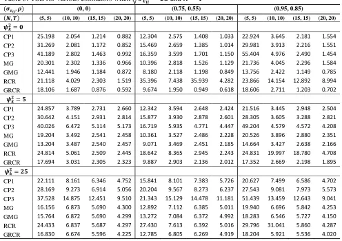
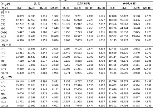
6.2. Monte Carlo Results
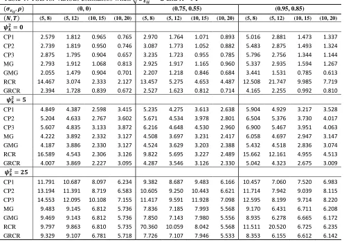
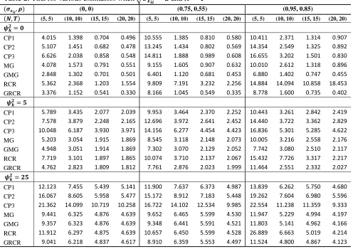
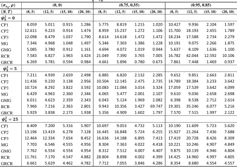
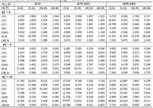
The results are given in Tables 1-6. Specifically, Tables 1-3 present the TSE values of the estimators when √ , and in cases of , , and , respectively. While case of
√ is presented in Tables 4-6 in the same cases of and . In our simulation study, the main
factors that have an effect on the TSE values of the estimators are , and . From Tables 1-6, we can summarize some effects for all estimators (classical pooling, random-coefficients, and mean group estimators) in the following points:
When the value of is increased, the values of TSE are increasing for all simulation situations.
When the values of and are increased, the values of TSE are decreasing for all situations.
When the value of is increased, the values of TSE are increasing in most situations.
02
1. In general, when , the TSE values of classical pooling estimators (CP1, CP2, and
CP3) are similar (approximately equivalent), especially when the sample size is moderate and/or
. However, the TSE values of GMG and GRCR estimators are smaller than the classical pooling estimators in this situation ( ) and other simulation situations (case of
and are increasing). In other words, the GMG and GRCR estimators are more
efficient than CP1, CP2, and CP3 estimators whether the regression coefficients are fixed (
) or random ( ).
2. Also, when the coefficients are random (when ), the values of TSE for GMG and GRCR estimators are smaller than MG and RCR estimators in all simulation situations (for any
and ). However, the TSE values of GRCR estimator are smaller than the values of TSE for GMG estimator in most situations, especially when the sample size is moderate. In other words, the GRCR estimator performs well than all other estimators as long as the sample size is moderateregardless of other simulation factors.
3. If , the values of TSE for MG and GMG estimators are approximately equivalent. This result is consistent with Lemma 2. According our study, the case of is achieved when the sample size is moderate in Tables 1, 2, 4 and 5. Moreover, that convergence is slowing down if and are increasing. But the situation for RCR and GRCR estimators is different; the convergence between them is very slow even if . So the MG and GMG estimators are more efficient than RCR estimator in all simulation situations.
4. Generally, the performance of all estimators in cases of and is better than their performance in case of . Similarly, Their performance in cases of √ is better than the performance in case of √ ,but it is not significantly as in and .
7. Conclusion
In this paper, the classical pooling (CP1, CP2, and CP3), random-coefficients (RCR and GRCR), and alternative (MG and GMG) estimators of stationary RCPD models were examined in different sample sizes in case the errors are cross-sectionally and serially correlated. Efficiency comparisons for these estimators indicate that the mean group and random-coefficients estimators are equivalent
when sufficiently large. Moreover, we carried out Monte Carlo simulations to investigate the small
samples performance for all estimators given above.
The Monte Carlo results show that the classical pooling estimators are not suitable for random-coefficients models absolutely. Also, the MG and GMG estimators are more efficient than RCR estimator in random- and fixed-coefficients models especially when is small ( ). Moreover, the GMG and GRCR estimators perform well in small samples if the coefficients are random or fixed.
The MG, GMG, and GRCR estimators are approximately equivalent when . However, the GRCR
03
Appendix
A.1 Proof of Lemma 1
a. Show that ( ̅̂ ) ( ̅̂ ) ̅
By substituting (25) into (29), we can get
̅̂ ∑ ( ) , (A.1)
by substituting into (A.1), then
̅̂ ∑ , ( ) -. (A.2)
Similarly, we can rewrite ̅̂ in (28) as:
̅̂ ∑ , ( ) -. (A.3)
Taking the expectation for (A.2) and (A.3), and using assumption 1, we get
( ̅̂ ) ( ̅̂ ) ∑ ̅.
b.Derive the variance-covariance matrix of ̅̂ :
Beginning, note that under assumption 8, we have ̅ . Let us add ̂ to the both sides:
̂ ̅ ̂
̂ ̅ ( ̂ ) (A.4) let ̂ then we can rewrite the equation (A.4) as follows:
̂ ̅ (A.5)
where ( ) . From (A.5), we can get
∑ ̂ ̅ ∑ ∑ ,
which means that
̅̂ ̅ ̅ ̅ (A.6)
where ̅ ∑ and ̅ ∑ . From (A.6) and using the general RCR assumptions, we get
( ̅̂ ) ( ̅) ( ̅)
∑ ( )
∑ ( ) ( )
(A.7)
Using the consistent estimators of and that defined in above, we get
̂ ( ̅̂ ) ( )
[
(∑ ̂ ̂
∑ ̂
∑ ̂
)
∑ ̂ ( ̂ ) ̂ ̂ ̂ ( ̂ )
04
c. Derive the variance-covariance matrix of ̅̂ :
As above, we can rewrite the equation (3) as follows:
̂ ̅ (A.8)
where ̂ ( ) . From (A.8), we can get
∑ ̂ ̅ ∑ ∑ ,
which means that
̅̂ ̅ ̅ ̅ (A.9)
where ̅ ∑ , and ̅ ∑ . From (A.9) and using the general RCR assumptions, we get
( ̅̂ ) ( ̅) ( ̅) ∑ ( ) ( ) ∑ ( ) ( ) . (A.10)
As in GMG estimator, by using the consistent estimators of and , we get
̂ ( ̅̂ ) ̂ ∑ ̂ ( ) ̂ ( ) ∑ ̂ ( ) ̂ ( )
.
A.2 Proof of Lemma 2:
Following the same argument as in Parks (1967) and utilizing assumption 10, we can show that
̂ ̂ ̂ ̂ , and
̂ (A.11) and then, ̂ ( ̂ ) ̂ ( ) ̂ ( ) ̂ ( ) ̂ ( ) ̂ ( ̂ ) ̂ ̂
̂ ( ̂ ) (A.12)
Substituting (A.11) and (A.12) in (24), we get
̂ .∑ ∑ ∑ / . (A.13)
By substitute (A.11)-(A.13) into (30), (31), and (27), we get
̂ ( ̅̂ ) ̂ ∑ ̂ ( ) ̂ ( ) ∑ ̂ ( ) ̂ ( )
, (A.14)
̂ ( ̅̂ )
( ) .∑ ̂ ̂ ∑ ̂ ∑ ̂ /
( )∑ 0 ̂ ( ̂ ) ̂ ̂ ̂ ( ̂ )
1
, (A.15)
̂ ( ̅̂ ) ( ̂
) [∑ ]
05
Similarly, we will use the results in (A.11)-(A.13) in case of RCR estimator:
̂ ( ̅̂ ) 0( ̂
) ̂ ̂ ̂ ( ̂ ) 1 . (A.17)
From (A.14)-(A.17), we can conclude that:
̂ ( ̅̂ ) ̂ ( ̅̂ ) ̂ ( ̅̂ ) ̂ ( ̅̂ ) .
References
Abonazel, M. R. (2009). Some Properties of Random Coefficients Regression Estimators. MSc thesis. Institute of Statistical Studies and Research. Cairo University.
Abonazel, M. R. (2014). Some estimation methods for dynamic panel data models. PhD thesis. Institute of Statistical Studies and Research. Cairo University.
Alcacer, J., Chung, W., Hawk, A., Pacheco-de-Almeida, G. (2013). Applying random coefficient models to strategy research: testing for firm heterogeneity, predicting firm-specific coefficients, and estimating Strategy Trade-Offs.Working Paper, No. 14-022. Harvard Business School Strategy Unit.
Anh, V. V., Chelliah, T. (1999). Estimated generalized least squares for random coefficient regression models. Scandinavian journal of statistics 26(1):31-46.
Baltagi, B. H. (2011). Econometrics. 5th ed. Berlin: Springer-Verlag Berlin Heidelberg.
Baltagi, B. H. (2013). Econometric Analysis of Panel Data. 5th ed. Chichester: John Wiley and Sons.
Beck, N., Katz, J. N. (2007). Random coefficient models for time-series–cross-section data: Monte Carlo experiments. Political Analysis 15(2):182-195.
Beran, R., Millar, P. W. (1994). Minimum distance estimation in random coefficient regression models. The Annals of Statistics 22(4):1976-1992.
Bodhlyera, O., Zewotir, T., Ramroop, S. (2014). Random coefficient model for changes in viscosity in dissolving pulp. Wood Research 59(4):571-582.
Boness, A. J., Frankfurter, G. M. (1977). Evidence of Non-Homogeneity of capital costs within “risk-classes”. The Journal of Finance 32(3):775-787.
Boot, J. C., Frankfurter, G. M. (1972). The dynamics of corporate debt management, decision rules, and some empirical evidence. Journal of Financial and Quantitative Analysis 7(04):1957-1965.
Chelliah, N. (1998). A new covariance estimator in random coefficient regression model. The Indian Journal of Statistics, Series B 60(3):433-436.
Cheng, J., Yue, R. X., Liu, X. (2013). Optimal Designs for Random Coefficient Regression Models with Heteroscedastic Errors. Communications in Statistics-Theory and Methods 42(15):2798-2809.
Cooley, T. F., Prescott, E. C. (1973). Systematic (non-random) variation models: varying parameter regression: a theory and some applications. Annals of Economic and Social Measurement 2(4): 463-473.
Dielman, T. E. (1983). Pooled cross-sectional and time series data: a survey of current statistical methodology.
The American Statistician 37(2):111-122.
Dielman, T. E. (1989). Pooled Cross-Sectional and Time Series Data Analysis. New York: Marcel Dekker.
Dielman, T. E. (1992a). Misspecification in random coefficient regression models: a Monte Carlo simulation.
Statistical Papers 33(1):241-260.
Dielman, T. E. (1992b). Small sample properties of random coefficient regression estimators: a Monte Carlo simulation. Communications in Statistics-Simulation and Computation 21(1):103-132.
Dwivedi, T.D., Srivastava, V.K. (1978). Optimality of least squares in the seemingly unrelated regression equation model. Journal of Econometrics 7:391-395.
Dziechciarz, J. (1989). Changing and random coefficient models. A survey. In: Hackl, P., ed. Statistical Analysis and Forecasting of Economic Structural Change. Berlin: Springer Berlin Heidelberg.
06
Elster, C., Wübbeler, G. (2016). Bayesian inference using a noninformative prior for linear Gaussian random coefficient regression with inhomogeneous within-class variances. Computational Statistics (in press). DOI: 10.1007/s00180-015-0641-3.
Feige, E. L., Swamy, P. A. V. B. (1974). A random coefficient model of the demand for liquid assets. Journal of Money, Credit and Banking, 6(2):241-252.
Fu, K. A., Fu, X. (2015). Asymptotics for the random coefficient first-order autoregressive model with possibly heavy-tailed innovations. Journal of Computational and Applied Mathematics 285:116-124.
Horváth, L., Trapani, L. (2016). Statistical inference in a random coefficient panel model. Journal of Econometrics 193(1):54-75.
Hsiao, C. (2014). Analysis of Panel Data. 3rd ed. Cambridge: Cambridge University Press.
Hsiao, C., Pesaran, M. H. (2008). Random coefficient models. In: Matyas, L., Sevestre, P., eds. The Econometrics of Panel Data. Vol. 46. Berlin: Springer Berlin Heidelberg.
Judge, G. G., Griffiths, W. E., Hill, R. C., Lütkepohl, H., Lee, T. C. (1985). The Theory and Practice of Econometrics, 2nd ed. New York: Wiley.
Livingston, M., Erickson, K., Mishra, A. (2010). Standard and Bayesian random coefficient model estimation of US Corn–Soybean farmer risk attitudes. In Ball, V. E., Fanfani, R., Gutierrez, L., eds. The Economic Impact of Public Support to Agriculture. Springer New York.
Mousa, A., Youssef, A. H., Abonazel, M. R. (2011). A Monte Carlo study for Swamy’s estimate of random
coefficient panel data model. Working paper, No. 49768. University Library of Munich, Germany.
Murtazashvili, I., Wooldridge, J. M. (2008). Fixed effects instrumental variables estimation in correlated random coefficient panel data models. Journal of Econometrics 142:539-552.
Parks, R. W. (1967). Efficient Estimation of a System of regression equations when disturbances are both serially and contemporaneously correlated. Journal of the American Statistical Association 62:500-509.
Pesaran, M.H., Smith, R. (1995). Estimation of long-run relationships from dynamic heterogeneous panels.
Journal of Econometrics 68:79-114.
Poi, B. P. (2003). From the help desk: Swamy’s random-coefficients model. The Stata Journal 3(3):302-308. Rao, C. R. (1973). Linear Statistical Inference and Its Applications. 2nd ed. New York: John Wiley & Sons. Rao, C. R., Mitra, S. (1971). Generalized Inverse of Matrices and Its Applications.John Wiley and Sons Ltd. Rao, U. G. (1982). A note on the unbiasedness of Swamy's estimator for the random coefficient regression
model. Journal of econometrics 18(3):395-401.
Rausser, G.C., Mundlak, Y., Johnson, S.R. (1982). Structural change, updating, and forecasting. In: Rausser, G.C., ed. New Directions in Econometric Modeling and Forecasting US Agriculture. Amsterdam: North-Holland. Sant, D. (1977). Generalized least squares applied to time-varying parameter models. Annals of Economic and
Social Measurement 6(3):301-314.
Srivastava, V. K., Giles, D. E. A. (1987). Seemingly Unrelated Regression Equations Models: Estimation and Inference. New York: Marcel Dekker.
Swamy, P. A. V. B. (1970). Efficient inference in a random coefficient regression model. Econometrica 38:311-323.
Swamy, P. A. V. B. (1971). Statistical Inference in Random Coefficient Regression Models. New York: Springer-Verlag.
Swamy, P. A. V. B. (1973). Criteria, constraints, and multicollinearity in random coefficient regression model.
Annals of Economic and Social Measurement 2(4):429-450.
Swamy, P. A. V. B. (1974). Linear models with random coefficients. In: Zarembka, P., ed. Frontiers in Econometrics. New York: Academic Press.
Swamy, P. A. V. B., Mehta, J. S., Tavlas, G. S., Hall, S. G. (2015). Two applications of the random coefficient procedure: Correcting for misspecifications in a small area level model and resolving Simpson's paradox. Economic Modelling 45:93-98.
Westerlund, J., Narayan, P. (2015). A random coefficient approach to the predictability of stock returns in panels. Journal of Financial Econometrics 13(3):605-664.
07
Youssef, A. H., Abonazel, M. R. (2015). Alternative GMM estimators for first-order autoregressive panel model: an improving efficiency approach. Communications in Statistics-Simulation and Computation (in press). DOI: 10.1080/03610918.2015.1073307.
Youssef, A. H., El-sheikh, A. A., Abonazel, M. R. (2014a). Improving the efficiency of GMM estimators for dynamic panel models. Far East Journal of Theoretical Statistics 47:171–189.
Youssef, A. H., El-sheikh, A. A., Abonazel, M. R. (2014b). New GMM estimators for dynamic panel data models.
International Journal of Innovative Research in Science, Engineering and Technology 3:16414–16425. Zellner, A. (1962). An efficient method of estimating seemingly unrelated regressions and tests of aggregation
08
Table 1: TSE for various estimators when √and
( ) (0, 0) (0.75, 0.55) (0.95, 0.85)
( ) (5, 8) (5, 12) (10, 15) (10, 20) (5, 8) (5, 12) (10, 15) (10, 20) (5, 8) (5, 12) (10, 15) (10, 20)
CP1 2.579 1.812 0.965 0.765 2.970 1.764 1.071 0.893 5.016 2.881 1.473 1.337
CP2 2.739 1.819 0.950 0.746 3.087 1.773 1.052 0.882 5.483 2.875 1.493 1.324
CP3 2.875 1.795 0.904 0.657 3.235 1.723 0.955 0.785 5.796 2.756 1.344 1.144
MG 2.793 1.912 1.068 0.813 2.925 1.917 1.165 0.960 5.337 2.935 1.594 1.267
GMG 2.055 1.479 0.904 0.701 2.207 1.218 0.846 0.684 3.441 1.531 0.785 0.613
RCR 14.467 3.074 2.333 2.127 13.457 5.275 4.653 4.487 12.508 21.747 9.985 7.719
GRCR 2.394 1.728 0.839 0.672 2.527 1.623 0.812 0.714 4.165 2.255 0.992 0.810
CP1 4.849 4.387 2.598 3.415 5.235 4.275 3.613 2.638 5.904 4.929 3.217 3.528
CP2 5.204 4.633 2.767 3.602 5.671 4.534 3.978 2.801 6.504 5.376 3.730 4.017
CP3 5.607 4.835 3.133 3.872 6.216 4.648 4.530 2.960 6.900 5.467 3.951 4.063
MG 4.222 3.892 2.332 3.127 4.508 3.697 3.231 2.417 6.058 4.697 2.947 3.147
GMG 4.187 3.886 2.330 3.127 4.524 3.629 3.203 2.388 5.432 4.518 2.836 3.074
RCR 16.589 4.543 2.306 3.126 9.822 5.695 3.227 2.489 15.662 12.161 4.955 4.513
GRCR 4.007 3.869 2.227 3.095 4.287 3.546 3.126 2.330 5.042 4.323 2.675 3.009
CP1 11.791 10.687 8.097 6.234 9.382 8.687 9.483 6.166 10.457 7.060 7.520 6.983
CP2 13.194 11.391 8.719 6.583 10.605 9.250 10.443 6.621 11.714 7.942 9.039 8.115
CP3 14.553 12.095 10.108 7.155 11.417 9.591 11.928 7.098 12.595 8.199 9.714 8.220
MG 9.483 9.145 6.812 5.736 7.836 7.185 7.993 5.568 9.170 6.431 6.711 6.208
GMG 9.469 9.143 6.812 5.736 7.850 7.143 7.980 5.556 8.935 6.278 6.665 6.172
RCR 9.797 9.863 6.810 5.735 70.360 10.059 8.042 5.568 11.511 20.520 6.725 6.235
09
Table 2: TSE for various estimators when √and
( ) (0, 0) (0.75, 0.55) (0.95, 0.85)
( ) (5, 5) (10, 10) (15, 15) (20, 20) (5, 5) (10, 10) (15, 15) (20, 20) (5, 5) (10, 10) (15, 15) (20, 20)
CP1 4.015 1.398 0.704 0.496 10.555 1.385 0.810 0.580 10.411 2.371 1.314 0.907
CP2 5.107 1.451 0.682 0.478 13.245 1.434 0.802 0.569 14.354 2.549 1.325 0.892
CP3 6.626 2.038 0.858 0.548 14.811 1.888 0.989 0.608 16.655 3.202 1.501 0.830
MG 4.078 1.573 0.791 0.551 9.155 1.605 0.907 0.632 10.010 2.612 1.318 0.896
GMG 2.848 1.302 0.701 0.501 6.401 1.120 0.681 0.453 6.880 1.402 0.747 0.455
RCR 5.362 2.368 1.203 1.554 9.809 7.191 3.232 2.256 14.884 14.094 10.858 18.453
GRCR 3.376 1.152 0.541 0.330 8.166 1.045 0.549 0.335 8.778 1.600 0.735 0.402
CP1 5.789 3.435 2.077 2.039 9.953 3.464 2.370 2.252 10.443 3.261 2.842 2.419
CP2 7.578 3.879 2.248 2.165 12.696 3.972 2.641 2.452 14.440 3.722 3.362 2.829
CP3 10.048 6.187 3.930 3.971 14.156 6.277 4.454 4.423 16.836 5.301 5.285 4.622
MG 5.203 3.054 1.915 1.869 8.545 3.118 2.148 2.073 10.005 3.216 2.558 2.176
GMG 4.948 3.051 1.914 1.869 7.302 3.070 2.129 2.052 7.742 3.080 2.510 2.117
RCR 7.719 3.101 1.897 1.865 10.074 3.710 2.137 2.067 15.432 7.726 3.317 2.217
GRCR 4.762 2.823 1.809 1.812 7.761 2.876 2.023 1.999 11.464 2.551 2.332 2.027
CP1 12.123 7.455 5.439 5.141 11.900 7.637 6.373 4.987 13.839 6.262 5.750 4.680
CP2 16.067 8.605 5.958 5.477 15.172 8.912 7.183 5.448 19.262 7.604 6.980 5.596
CP3 21.362 14.099 10.719 10.258 16.722 14.102 12.534 9.985 22.554 11.238 11.359 9.333
MG 9.441 6.325 4.876 4.639 9.652 6.465 5.599 4.530 11.947 5.229 4.994 4.197
GMG 9.357 6.323 4.876 4.639 9.348 6.441 5.591 4.521 11.803 5.141 4.962 4.166
RCR 11.912 6.297 4.875 4.639 10.657 6.450 5.599 4.528 26.889 6.663 5.019 4.214
21
Table 3: TSE for various estimators when √and
( ) (0, 0) (0.75, 0.55) (0.95, 0.85)
( ) (8, 5) (12, 5) (15, 10) (20, 10) (8, 5) (12, 5) (15, 10) (20, 10) (8, 5) (12, 5) (15, 10) (20, 10)
CP1 8.059 5.011 0.915 1.286 5.775 8.819 1.215 1.020 10.427 9.936 2.104 1.597
CP2 12.611 9.223 0.914 1.474 8.959 15.237 1.272 1.106 15.700 18.193 2.455 1.789
CP3 12.098 8.479 1.037 1.790 8.614 14.618 1.472 1.472 18.234 17.588 2.734 2.279
MG 7.346 4.968 1.048 1.497 5.346 7.303 1.386 1.228 10.191 9.075 2.266 1.875
GMG 5.085 3.780 0.912 1.161 4.694 4.072 1.019 0.944 5.637 8.109 1.636 1.100
RCR 7.583 6.827 1.963 3.424 21.049 7.390 3.765 7.005 16.782 42.044 12.592 10.106
GRCR 6.269 3.781 0.594 0.984 4.661 5.896 0.780 0.673 7.861 7.448 1.469 0.937
CP1 7.211 4.939 2.659 2.498 6.885 6.820 2.132 2.285 9.652 9.851 2.663 2.811
CP2 11.436 9.220 3.138 2.956 10.504 12.145 2.475 2.735 14.789 18.384 3.233 3.642
CP3 10.724 8.292 3.822 3.592 10.083 11.084 3.014 3.324 17.059 17.539 3.642 4.099
MG 6.429 4.963 2.360 2.346 6.065 5.477 2.001 2.107 9.610 9.036 2.658 2.698
GMG 6.011 4.623 2.359 2.343 6.043 5.124 1.969 2.082 6.398 8.538 2.712 2.614
RCR 7.966 7.216 2.363 2.801 9.943 10.356 3.427 69.747 19.301 35.246 6.077 5.216
GRCR 5.929 3.838 2.173 1.938 5.356 4.909 1.602 1.797 7.570 7.515 1.997 2.122
CP1 8.409 7.200 5.316 5.907 10.697 9.053 4.732 5.113 10.190 11.609 5.723 5.620
CP2 13.196 13.419 6.278 7.128 16.445 16.848 5.724 6.255 15.927 21.264 7.436 7.688
CP3 12.464 12.334 7.654 8.452 16.636 14.188 6.895 7.413 17.419 20.728 8.426 8.309
MG 7.703 6.546 4.555 4.956 8.304 7.363 4.022 4.418 10.221 10.246 4.907 4.849
GMG 7.762 6.554 4.554 4.954 8.312 7.512 4.007 4.407 9.875 10.139 4.946 4.804
RCR 11.761 7.170 4.547 4.882 28.804 8.898 4.002 4.399 14.425 14.960 4.997 4.805
20
Table 4: TSE for various estimators when √and
( ) (0, 0) (0.75, 0.55) (0.95, 0.85)
( ) (5, 8) (5, 12) (10, 15) (10, 20) (5, 8) (5, 12) (10, 15) (10, 20) (5, 8) (5, 12) (10, 15) (10, 20)
CP1 4.700 2.869 1.578 1.344 6.294 2.990 1.827 1.522 9.733 4.994 2.793 2.177
CP2 4.854 2.876 1.564 1.316 6.823 3.020 1.805 1.502 10.431 5.022 2.758 2.167
CP3 5.109 2.822 1.505 1.178 7.166 2.941 1.667 1.339 10.790 4.959 2.460 1.880
MG 4.823 3.074 1.747 1.466 6.259 3.127 1.979 1.663 9.745 5.422 2.946 2.049
GMG 3.652 2.410 1.480 1.258 4.985 2.204 1.474 1.118 4.269 2.336 1.436 1.041
RCR 7.652 10.706 2.723 8.070 16.169 5.969 8.925 5.743 11.531 15.708 13.279 38.349
GRCR 4.324 2.725 1.389 1.191 5.674 2.717 1.502 1.202 7.352 3.872 1.801 1.320
CP1 6.069 4.812 3.119 3.565 6.382 3.283 4.274 4.306 8.993 4.950 3.200 3.396
CP2 6.311 4.969 3.279 3.720 6.996 3.349 4.619 4.615 9.682 5.095 3.271 3.745
CP3 6.704 5.101 3.651 3.948 7.415 3.290 5.165 4.883 9.905 5.076 3.151 3.664
MG 5.598 4.489 2.874 3.274 6.331 3.337 3.836 3.998 9.174 5.334 3.286 3.147
GMG 5.461 4.462 2.871 3.273 5.948 3.027 3.787 3.919 5.693 4.178 2.852 2.948
RCR 11.318 6.401 3.760 3.452 10.609 13.571 4.511 4.017 16.977 31.590 19.676 10.222
GRCR 5.476 4.308 2.659 3.143 5.996 3.116 3.581 3.829 7.382 4.398 2.430 2.770
CP1 11.783 10.693 8.316 7.119 13.570 8.748 7.442 7.734 8.176 14.887 7.895 6.279
CP2 12.614 11.288 8.920 7.496 14.942 9.425 8.219 8.342 9.083 16.391 9.390 7.273
CP3 13.791 11.705 10.160 8.070 15.989 9.956 9.417 9.007 9.310 16.943 10.113 7.413
MG 9.398 9.171 7.055 6.387 11.139 7.758 6.555 6.899 8.718 12.302 7.244 5.824
GMG 9.395 9.156 7.054 6.386 11.228 7.717 6.520 6.852 6.889 11.999 7.085 5.711
RCR 12.364 10.120 7.048 6.382 474.87
3
12.815 6.559 6.889 88.890 18.314 7.466 8.117
22
Table 5: TSE for various estimators when √and
( ) (0, 0) (0.75, 0.55) (0.95, 0.85)
( ) (5, 5) (10, 10) (15, 15) (20, 20) (5, 5) (10, 10) (15, 15) (20, 20) (5, 5) (10, 10) (15, 15) (20, 20)
CP1 25.198 2.054 1.214 0.882 12.304 2.575 1.408 1.033 22.924 3.645 2.181 1.554
CP2 31.269 2.081 1.172 0.852 15.469 2.659 1.385 1.014 29.981 3.913 2.216 1.551
CP3 41.189 2.802 1.463 0.992 16.359 3.599 1.701 1.150 55.404 4.976 2.490 1.454
MG 20.301 2.302 1.336 0.966 10.396 2.818 1.526 1.129 21.736 4.045 2.296 1.584
GMG 12.441 1.946 1.184 0.872 8.180 2.118 1.198 0.849 13.756 2.422 1.149 0.785
RCR 21.118 4.029 2.303 1.519 35.396 7.438 35.939 4.282 23.866 14.154 12.892 8.994
GRCR 18.106 1.687 0.876 0.592 9.674 1.950 0.949 0.618 18.606 2.711 1.203 0.702
CP1 24.857 3.789 2.731 2.660 12.342 3.594 2.648 2.424 21.516 3.445 2.948 2.504
CP2 30.642 4.151 2.931 2.814 15.877 3.930 2.878 2.601 28.305 3.605 3.288 2.821
CP3 40.026 6.472 5.114 5.173 16.719 5.935 4.771 4.447 49.204 4.579 4.572 4.208
MG 19.204 3.492 2.541 2.458 10.361 3.527 2.486 2.228 20.526 3.896 2.880 2.351
GMG 13.204 3.487 2.540 2.457 9.071 3.469 2.451 2.185 14.664 3.427 2.638 2.166
RCR 24.814 5.061 2.509 2.445 18.642 8.365 2.945 2.243 24.831 19.997 18.780 4.708
GRCR 17.694 3.031 2.305 2.323 9.887 2.903 2.136 2.012 17.352 2.669 2.198 1.895
CP1 22.111 8.161 6.346 4.752 15.841 8.101 7.383 5.726 20.627 7.499 6.586 4.702
CP2 28.169 9.273 6.914 5.056 20.204 9.567 8.273 6.237 27.543 9.081 7.973 5.573
CP3 37.528 14.875 12.451 9.510 21.343 15.129 14.478 11.181 51.439 13.459 12.643 9.041
MG 16.156 6.873 5.690 4.300 12.892 7.112 6.385 5.011 19.940 6.696 5.842 4.253
GMG 15.764 6.872 5.690 4.299 13.272 7.084 6.372 4.992 18.283 6.546 5.727 4.150
RCR 24.433 6.837 5.687 4.297 27.430 7.613 6.392 5.016 29.796 31.041 5.860 4.287
23
Table 6: TSE for various estimators when √and
( ) (0, 0) (0.75, 0.55) (0.95, 0.85)
( ) (8, 5) (12, 5) (15, 10) (20, 10) (8, 5) (12, 5) (15, 10) (20, 10) (8, 5) (12, 5) (15, 10) (20, 10)
CP1 8.099 17.393 1.731 1.392 10.036 9.281 2.099 1.675 12.098 58.422 3.198 2.578
CP2 12.381 32.968 1.781 1.406 16.362 16.928 2.229 1.727 18.230 95.939 3.496 2.705
CP3 12.232 29.385 2.033 1.963 18.922 15.942 2.556 2.392 19.356 93.663 3.873 3.693
MG 7.742 14.751 2.034 1.648 10.003 9.046 2.453 1.892 10.226 44.144 3.628 2.836
GMG 5.447 9.402 1.768 1.463 6.250 7.273 2.045 1.736 10.228 38.853 2.075 1.775
RCR 8.382 17.489 3.876 10.630 15.198 48.547 6.812 46.391 20.562 48.053 19.644 21.881
GRCR 6.386 12.973 1.153 0.834 8.263 7.059 1.423 1.010 9.115 37.422 1.908 1.403
CP1 7.977 15.698 3.145 2.695 9.307 9.106 2.874 2.892 12.425 55.988 3.053 2.948
CP2 12.251 29.797 3.544 3.100 15.449 16.513 3.210 3.379 18.659 92.529 3.340 3.272
CP3 12.069 26.622 4.361 3.805 17.208 15.601 3.799 4.140 20.114 89.044 3.635 4.271
MG 7.550 12.435 2.977 2.522 9.329 8.838 2.927 2.704 10.485 42.576 3.558 3.085
GMG 6.193 9.803 2.975 2.520 7.059 7.670 2.915 2.731 10.795 37.501 3.151 2.916
RCR 9.369 15.712 3.497 2.553 12.705 21.261 3.835 2.992 18.461 47.773 26.250 22.414
GRCR 6.490 11.975 2.384 1.995 8.071 6.935 2.060 2.101 9.445 35.999 2.038 1.799
CP1 10.148 14.075 6.294 5.831 9.455 9.717 6.780 5.270 13.786 57.674 6.578 5.433
CP2 15.623 26.924 7.411 6.918 15.729 17.896 8.220 6.437 20.662 91.990 8.384 7.082
CP3 15.672 23.191 9.144 8.111 17.441 17.000 9.768 7.650 22.626 91.419 9.488 7.981
MG 9.006 11.305 5.418 4.844 9.752 9.346 5.856 4.467 11.409 43.289 6.030 4.925
GMG 8.838 11.598 5.417 4.843 8.971 9.206 5.853 4.489 11.916 38.975 5.877 4.826
RCR 11.771 13.046 5.377 4.813 14.957 11.915 5.896 4.437 21.958 42.733 8.370 4.872