Recent Modifications of Adomian Decomposition
Method for Initial Value Problem in Ordinary
Differential Equations
M. Almazmumy, F. A. Hendi, H. O. Bakodah, H. Alzumi
Department of Mathematics, Science Faculty for Girls, King Abdulaziz University, Jeddah, KSA Email: [email protected], [email protected], [email protected], [email protected]
Received May 12,2012; revised June 20, 2012; accepted July 1, 2012
ABSTRACT
In this paper, some modifications of Adomian decomposition method are presented for solving initial value problems in ordinary differential equations. Also, the restarted and two-step methods are applied to the problem. The effectiveness of the each modified is verified by several examples.
Keywords: Adomian Decomposition Method; Initial Value Problem; Modified Adomian Decomposition Method
1. Introduction
Recently a great deal of interest has been focused on the application of Adomian’s decomposition method to solve a wide variety of linear and nonlinear problems [1]. This method generates a solution in the form of a series whose terms are determined by a recursive relationship using the Adomian polynomials. Researchers who have used the ADM have frequently enumerated on the many ad-vantages that it offers. Since it was first presented in the 1980’s, Adomian decomposition method has led to sev-eral modifications on the method made by various re-searchers in an attempt to improve the accuracy or ex-pand the application of the original method. Adomian and Rach [2] introduced modified Adomian polynomials which converge slightly faster than the original polyno-mials and are convenient for computer generation. Ado- mian also introduced accelerated Adomian polynomials [3], despite the various types of Adomian polynomials available, the original Adomian polynomials are more generally used based on the advantage of a convenient algorithm which is easily remembered. Recently, F. A. Hendi et al. [4] presented simple Mathematica program to compute Adomian polynomials. Wazwaz [5] used padé approximants to the solution obtained using a mo- dified decomposition method and found that not only does this improve the result, but also that the error de-creases with the increase of the degree of the padé ap-proximants. Another modification to ADM was proposed by Wazwaz [6] a reliable modification of the Adomian decomposition method. In 2005, Wazwaz [7] presented another type of modification to the ADM. New
modifi-cation was proposed by Luo [8,9], this variation sepa-rates the ADM into two steps and therefore is termed the two-step ADM or ( TS ADM ). Another recent modifica-tion is termed the restarted Adomian method [10,11], this method involves repeatedly updating the initial term of the series generated.
Several other researchers have developed modifica-tions to the ADM [12-17]. The modificamodifica-tions arise from evaluating difficulties specific for the type of problem under consideration. The modification usually involves only a slight change and is aimed at improving the con-vergence or accuracy of the series solution. The main goal of this paper is to apply some modifications of Adomian decomposition method to the initial value problem in ordinary differential equation and compare the results of an original ADM to those with the modifi-cations. As we know, we point out that restarted and two-step methods are applied on the initial value problem for the first time. Our numerical examples show which of these methods give best results.
2. A General Description of the ADM
A general nonlinear differential equation will be used for simplicity, we consider
Fy f
where F is a nonlinear differential operator and y and f are functions of x. Rewriting the equation in the operator form
F which easily invertible, R is a linear operator for the reminder of the linear portion, and N is a nonlinear op-erator representing the nonlinear term in F.
Applying the inverse operator , the equation then becomes
1
L
1 1 1 1
L Ly L f L Ry L Ny
since F was taken to be a differential operator and L is linear, would represents an integration and with any given initial conditions, will give an equation for y incorporating these conditions. This gives
1
L
1
L Ly
1 1y x g x L Ry L Ny (2) where g x
represents the function generated by inte-grating f and using the initial conditions.Adomian decomposition method admits the decompo-sition into an infinite series of components
0 n
n
y x y x
(3)The nonlinear term be equated to an infinite se-ries polynomial
Ny
0 n
n
Ny A
(4)n
A is the Adomian polynomials, which can be deter-mined by
0
1 d
! d n
n n
A Ny
n
0 n
n
(5)
substituting (4) and (5) into (2)
1 10
0 n 0 n
n n
y x y L Ry L A
the recursive relationship is found to be
0 1 1
n n
y g x y L Ry L
1
n
A
0
(6)
Having determined the components , the so-lution y in a series form follows immediately. The series may be summed to provide the solution in a closed form. However, for concrete problems, the n-term partial sum may be used to give the approximate solution.
, n
y n
2.1. Convergence Analysis
The concept of convergence of the solution obtained by Adomian decomposition method was addressed by [1,18], and extensively by [19,20]. Convergence of the ADM when applied to initial value problem in ordinary differ-ential equation is discussed by many authors. For exam-ple, K. Abbaoui and Y. Cherruault [21,22]. In [23] H. Alzumi et al. discussed the convergence of ADM.
2.2. The Noise Terms Phenomenon
In this section, we will present a useful tool that will ac-celerate the convergence of the Adomian decomposition method. The noise terms phenomenon provides a major advantage in that it demonstrate a fast convergence of the solution. A useful summary about the noise terms phe-nomenon can be drawn as follows:
The noise terms are defined as the identical terms with opposite signs that may appear in the compo-nents y0 and y1.
The noise terms appear only for specific types of in-homogeneous equations whereas noise terms do not appear for homogeneous equations.
Noise terms may appear if the exact solution is part of the zeroth component y0.
Verification that the remaining non-canceled terms satisfy the equation is necessary and essential.
For further reading about the noise terms phenomenon see [24-27].
3. Some Recent Modifications of ADM
Several authors have proposed a variety of modifications to ADM. The modifications arise from evaluating diffi-culties specific for the type of problem under considera-tion. We begin with the Adomian’s modificaconsidera-tion.
3.1. Modified Adomian Method (M1): [1,28]
Power series solutions of linear homogeneous differential equation in initial-value problems yield simple recur-rence relations for the coefficient, but they are generally not adequate for nonlinear equations, although applicable to some simple cases such as the Riccati equation. To clarify the procedure, consider the general inhomogene- ous nonlinear form (1), where L will be chosen as
2
2 d dx , and operate with 1
We now have0 0 . x x . d L
t td .
0
0 1 1 1y y y xL f L Ry L Ny (7) Let
0
n n n
y c x
,0
n n n
f f x
, and (8)0
n n n
Ny A x
Now from (8) in (7), we obtain
1
0 0
1 1
0 0
1 0
0 0
0 0
1 2
n n
n n
n n
n n
n n
n n
n
n n n
n
c x y y x L f x
L R c x L A x
y y x
x f Rc A
n n
or
0 1 2
2 2 2
2
0 0
1
n n n
n
n n n
n
c c x c x y y x
x
f Rc A
n n
Equating coefficients, leading to:
0
1
2 2 2
0 0
, 2 1
n n n
n
c y c y
f Rc A
c n
n n
(9)
where An A c cn
0, , ,1 cn
.3.2. Wazwaz Modifications
3.2.1. Reliable Modification (M2): [6,29]
The reliable modification form based on the assumption that the function g in (2) can be divided into two parts, i.e.
0 1
gg g (10) Accordingly, a slight variation was proposed only on the components 0 and 1. The suggestion was that only the parts 0
y y
g be assigned to the component 0, whereas the remaining part
y 1
g be combined with other terms given in (6) to define . Consequently, the recur-sive relation, 1
y
0 0
1 1
1 1 0 0
1 1
2 1 1 , 0
n n n
y g
y g L Ry L A
y L Ry L A n
(11)
Although this variation in the formation of 0 and 1 is slight, however it plays a major role in accelerating the convergence of the solution and in minimizing the size of calculations.
y y
Furthermore, there is no need sometimes to evaluate the so-called Adomian polynomials required for nonlin-ear operators. Two important remarks related to the modified method were made in [6]. First, by proper se-lection of the function g0 and g1, the exact solution y may be obtained by using very few iterations, and some-times by evaluating only two components. The success of this modification depends only on the choice of g0 and
1
g , and this can be made through trials, that are the only criteria which can be applied so far.
Second, if g consists of one term only, the standard decomposition method should be employed in this case.
3.2.2. The New Modification (M3): [30]
As indicated earlier, although the modified decomposi-tion method may provide the exact soludecomposi-tion by using two iterations only, and sometimes without any need for
Adomian polynomials, but its effectiveness depends on the proper choice of g0 and g1. In the new modifica-tion, Wazwaz replaces the process of dividing g into two components by a series of infinite components. He
sug-sts that g be expressed in Taylor series ge
0
n n
g g
(12)Moreover, he suggest a new recursive relationship ex-pressed in the form
0 0
1 1
1 1 , 0
n n n n
y g
y g L Ry L A n
(13) It is important to note that if g consists of one term only, then scheme (13) reduces to relation (6). Moreover, if g consists of two terms, then relation (13) reduces to the modified relation (11). It is easily observed that algo-rithm (13) reduces the number of terms involved in each component, and hence the size of calculations is mini-mized compared to the standard Adomian decomposition method only. Moreover, this reduction of terms in each component facilitates the construction of Adomian poly-nomials for nonlinear operators.
3.3. Restarted Adomian Method (M4): [10,11]
The restarted ADM was used in [10] as a new method based on standard ADM for solving algebraic equations. In [11], E. Babolian et al. applied the restarted Adomian method to nonlinear integral equations and nonlinear integro-differential equations. The author in [31] applied the method to solve a system of nonlinear Fredholm in-tegral equations of the second kind.
In this method, we use the modified Adomian method which proposed a slight variation only on the compo-nents 0 and 1, and restarted Adomian method ap-plied to algebraic equations. The rate of the method is more accelerate than standard adomian method. If we consider a general nonlinear equation of the form (1) and applied ADM to solve it we get the recursive relationship (6), we introduce the algorithm of restarted Adomian method as the following:
y y
Choose small natural numbers m k, .
Apply the Adomian method on Equations (6) and cal-culate y y y0, , , ,1 2 yk
y y
Set 0 1 yk
Let Z be the proper function which will be determined next for j2 :m, j 1
Z 0
1 0
2 1
1
0 1 2
k k
j
k
y Z
y f Z A
y A
y A
y y y y
Remarks:
m can be considered as an approximation of (1).
The Adomian method usually gives sum of the some first terms as an approximation of y, in this algorithm we can update y0 in each step, but we don’t calcu-late the terms with large index, so m and k are con-sidered small.
3.4. Two-Step Adomian Method (M5): [8,9]
The Two-step Adomian decomposition method (TSADM) is derived by separate the standard ADM into two steps. The main ideas of two-step Adomian decomposition method for the differential Equation (1), are:
Applying the inverse operator to f, and using the given conditions, we obtain
1
L
1
L f
where the function represents the terms arising from using the given conditions, all are assumed to be pre-scribed.
To achieve the objectives of this study, we set
0 1 m
Based on this, we define
0 k k
y s
k
.
where k0,1, , , m s0,1, , m .
Then, we verify that 0 satisfies the original equation and the given conditions by substitution, once the exact solution is obtained we finish. Otherwise, we go to the following step two.
y
We set 0 and continue with the standard Ado- mian recursive relation y
1 1
1 , 0
n n n
y L Ry L A n
Compared to the standard Adomian method and the modified method, we can see that the two-step Adomian method may provide the solution by using one iteration only. Further, the (TSADM) avoids the difficulties aris-ing in the modified method. Furthermore, the number of the terms in namely m, is small in many practical problems.
4. Numerical Examples
In this section, some initial value problems are consid-ered to show the efficiency of each modified.
Example 1
cos sin sin , 0 0
y y x xx x x y MS (Standard Adomian Method):
Applying 1 to both sides yields L
sin cos sin 1
y x x xx x xL y x
The recursive relationship 0
1 1
sin cos sin
, 0
n n
y x x x x x
y L y n
So
1
1 0 cos sin sin 2 cos 1
y L y x x xx x x
Other components can be evaluated in a similar man-ner. It is easily observed that the noise terms
xcosx
and
sinx
appear in 0 and 1 with opposite signs. Canceling these noise terms from 0 gives the exact solutiony y
y
siny x x x that can be justified through substitution. It is worth noting that other noise terms that appear in other components vanish in the limit.
M1: Let
,
n n
n n
y
c x f
f xThen
0
1 1
0
, 1
n n
n
c
f c
c n
n
So that
2 4 6 3 5 sin3! 5! 3! 5!
x x x x
y x x x x x
x
M2:
0
1
1 0
1 1
sin
cos sin 0
0, 0
n n
y x x
y x x x L y
y L y n
Then the exact solution is y x
xsinxM3: The Taylor expansion for
sin cos sinf x x xx x x is given by
2 2 3 4 4 5 6 3! 3! 5! 5!x x x x
f x x
Then the recursive relationship 2 0
3 1
1 0
4 4
1
2 1
3 6
4
2 0
3!
3! 3!
0
5! y x
x
y L y
x x
y L y
y x y
2 4 6 3 5 sin3! 5! 3! 5!
x x x x
y x x x x x
x
M4: Let
0
1
1 0
sin
cos sin 0
y x x
y x x x L A Then 1 sin x x
Then the exact solution is yxsinx.
M5: Let
0 1 2
0 xsin ,x 1 xcos ,x 2 sin
x
Clearly 0, 1 and 2 satisfy , by selecting 0 0
0 0y
y and by verifying that justified the differen-tial equation. 0
y
Then, the exact solution is obtained immediately
sin
yx x.
Example 2
Consider nonlinear initial value problem
cos tan , 0 0
y
y e x x y
With the exact solution yln cosx.
Ms:
1 1
1 cos tan sin ln cos
y y
y L x x L e
x x L e
n
A s is Adomian polynomials of nonlinear term ey
0 0 0 1 0 1 1 2 2 1 1 2! y y y A e A y e
A y y e
with standard ADM, we obtained the recursive relation-ship
0 0 01 1 sin
1 0
1 1 2sin sin
2 1 1
sin ln cos
1
1 1 1
2
y x
y x x
y x x
y L A L e e
y L A L y e e e
n nIt is easy to see that the standard Adomian decomposition method converges to the exact solution very slowly, com- parison of absolute errors between the exact solution and approximate solutions Ms introduce in Table 1 and Fig-ure 1.
M1: Let
0 0 0
, ,
n n y
n n
n n n
y c x f f x e A x
Then
1 1
0 0 0
1
0 1
1 1 1
n n n
n n n
n n n
n n
n
n n n
n n n
c x L f x L A x
1
x x
c c x f L A
n n
So 0 1 1 0 , 0 n n n c f A c n n From this relation we get
3 5 7
1 1
2 4 6
2 3 4 5 6
3! 5! 7!
2 16
2 4! 6!
2 16
2 3! 4! 5! 6! 7!
n n n
x x x x
f f x
n
x x x
7
x x x x x x
x
This yield0 2 2 3
1 1
1, 1, , ,
2 3
f f f f
So the c si coefficients
0 0 0 1 1 1 2 3 4 0
1 1 0 1 1 2 2 0 2 4 c f A c f A c c c
The series solution obtained as
0
n n n
y c x
2 4
2 ln cos
2 4!
x x
y x
M2: gln cosxsin ,x g0ln cos ,x g1sinx 0
1 1 ln co
1 0
ln cos
sin sin 0
0, 2
x
n
y x
y x L A x L e
y n s
Then yln cosx.
M3:
3 5 7 2 4 6
2 3 4 5
sin ln cos
2 16
3! 5! 7! 2 4! 6!
2
2 3! 4! 5!
g x x
x x x x x x
x
x x x x
Table 1. Comparison of absolute errors between the exact solution and approximate solutions Ms and M3.
t Me Ms M3 Es E3
0.0 0.0 3.10862 × 10⁻¹⁵ 0.0 3.10862 × 10⁻¹⁵ 1.54811 × 10⁻¹¹
0.1 −0.00500836 −0.00500836 −0.00500836 1.48548 × 10⁻¹¹ 1.9028 × 10⁻⁹
0.2 −0.0201348 −0.0201348 −0.0201348 2.19203 × 10⁻⁸ 7.46429 × 10⁻⁷
0.3 −0.0456917 −0.0456934 −0.0456917 1.75982 × 10⁻⁶ 2.90542 × 10⁻⁵
0.4 −0.082229 −0.0822708 −0.082229 4.18148 × 10⁻⁵ 4.39705 × 10⁻⁴
0.5 −0.130584 −0.131082 −0.130584 4.98158 × 10⁻⁴ 3.96416 × 10⁻³
0.1 0.2 0.3 0.4 0.5
0.12 0.10 0.08 0.06 0.04 0.02
exacty
Ms
t
1
0 1 ln cos
y y x
Then the exact solution is yln cosx.
M5: Let
1 2
1 2
sin ln cos ln cos , sin
x x
x x
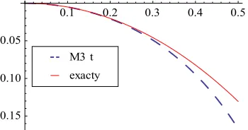
[image:6.595.86.261.370.462.2]Clearly 1 satisfy y
0 0 and by verifying that 1 justified the differential equation.Figure 1. Comparison between the exact solution and
ap-proximate solutions Ms. Hence, 1 ln cosx is the exact solution.
0.1 0.2 0.3 0.4 0.5
0.15 0.10 0.05
exacty
M3
t
REFERENCES
[1] G. Adomian, “Solving Frontier Problems of Physics: The Decomposition Method,” Springer, New York, 1993. [2] G. Adomian and R. Rach, “Modified Adomian
Polyno-mials,” Mathematical and Computer Modelling, Vol. 24, No. 11, 1996, pp. 39-46.
[3] Y. Cherruault, G. Adomian, K. Abbaoui and R. Rach, “Further Remarks on Convergence of Decomposition Method,” International Journal of Bio-Medical Comput-ing, Vol. 38, No. 1, 1995, pp. 89-93.
doi:10.1016/0020-7101(94)01042-Y Figure 2. Comparison between the exact solution and
ap-proximate solutions M3.
Then [4] F. A. Hendi, H. O. Bakodah, M. Almazmumy and H.
Alzumi, “A Simple Program for Solving Nonlinear Initial Value Problem Using Adomian Decomposition Method,”
International Journal of Research and Reviews in Applied Sciences, Vol. 12, No. 3, 2012.
0
2 2
1
1 0
3 2
1
2 1
1
2! 2!
3 1
3! 3! 2
1
1 1
2
x
x
x x
y x
x x
y L A e
x x x
y L A e x
e e
[5] A.-M. Wazwaz, “The Modified Decomposition Method and Padé Approximants for Solving the Thomas-Fermi Equation,” Applied Mathematics and Computation, Vol.
105, No. 1, 1999, pp. 11-19. doi:10.1016/S0096-3003(98)10090-5
[6] A.-M. Wazwaz, “A Reliable Modification of Adomian Decomposition Method,” Applied Mathematics Computa-tion, Vol. 102, No. 1, 1999, pp. 77-86.
doi:10.1016/S0096-3003(98)10024-3 The comparison of absolute errors between the exact
solution and approximate solution M3 introduce in Table
1 and Figure 2. [7] A.-M. Wazwaz, Adomian Decomposition Dethod for a
Deliable Dreatment of the Edman-Flower Dquation,” Ap- plied Mathematics and Computation, Vol. 161, No. 2, 2005, pp. 543-560. doi:10.1016/j.amc.2003.12.048
M4: Let
0
1
1 0
ln cos
sin 0
y x
y x L A
[8] X.-G. Luo, “A Two-Step Adomian Decomposition Me-
thod,” Applied Mathematics and Computation, Vol. 170,
[9] B.-Q. Zhang, Q.-B. Wu and X.-G. Luo, “Experimentation with Two-Step Adomian Decomposition Method to Solve Evolution Models,” Applied Mathematics and Computa-tion, Vol. 175, No. 2, 2006, pp. 1495-1502.
doi:10.1016/j.amc.2005.08.029
[10] E. Babolian and S. Javadi, “Restarted Adomian Method for Algebraic Equations,” Applied Mathematics and Com- putation, Vol. 146, No. 2-3, 2003, pp. 533-541.
doi:10.1016/S0096-3003(02)00603-3
[11] E. Babolian, S. Javadi and H. Sadehi, “Restarted Ado- mian Method for Integral Equations,” Applied Mathema- tics and Computation, Vol. 153, No. 2, 2004, pp. 353-359. doi:10.1016/S0096-3003(03)00636-2
[12] C. Jin and M. Liu, “A New Modification of Adomian Decomposition Method for Solving a Kind of Evolution Equations,” Applied Mathematics and Computation, Vol.
169, No. 2, 2005, pp. 953-962. doi:10.1016/j.amc.2004.09.072
[13] H. Jafari and V. Daftardar-Gejji, “Revised Adomian De- composition Method for Solving a System of Nonlinear Equations,” Applied Mathematics and Computation, Vol.
175, No. 1, 2006, pp. 1-7. doi:10.1016/j.amc.2005.07.010 [14] H. Jafari and V. Daftardar-Gejji, “Revised Adomian De-Composition Method for Solving a System of Ordinary and Fractional Differential Equations,” Applied Mathe-matics and Computation,” Vol. 181, No. 1, 2006, pp.
598-608. doi:10.1016/j.amc.2005.12.049
[15] M. M. Hosseini and H. Nasabzadeh, “Modified Adomian Decomposition Method for Specific Second Order Ordi-nary Differential Equations,” Applied Mathematics and Computation, Vol. 186, No.1, 2007, pp. 117-123.
doi:10.1016/j.amc.2006.07.094
[16] Y. Q. Hasan and L. M. Zhu, “Modified Adomian De-composition Method for Singular Initial Value Problems in the Second Order Ordinary Differential Equations,”
Surveys in Mathematics and Its Applications, Vol. 3,
2008, pp. 183-193.
[17] P. Pue-on and N. Viryapong, “Modified Adomian De-composition Method for Solving Particular Third-Order Ordinary Differential Equations,” Applied Mathematical Science, Vol. 6, No. 30, 2012, pp. 1463-1469.
[18] G. Adomian, “Nonlinear Stochastic Operator Equata- ions,” Academic Press, San Diego, 1986.
[19] Y. Cherruault, “Convergence of Adomians Method,” Ky- bernetes, Vol. 18, No. 2, 1989, pp. 31-38.
doi:10.1108/eb005812
[20] Y. Cherruault and G. Adomian, “Decomposition Method: A New Proof of Convergence,” Mathematical and
Com-puter Modelling, Vol. 18, No. 12, 1993, pp.103-106.
doi:10.1016/0895-7177(93)90233-O
[21] K. Abbaoui and Y. Cherruault, “Convergence of Ado- mian’s Method Applied to Differential Equations,” Com- puters & Mathematics with Applications, Vol. 28, No. 5,
1994, pp. 103-109. doi:10.1016/0898-1221(94)00144-8 [22] K. Abbaoui and Y. Cherruault, “Convergence of Ado-
mian Method Applied to Nonlinear Equations,” Mathe- matical and Computer Modelling, Vol. 20, No. 9, 1994,
pp. 69-73. doi:10.1016/0895-7177(94)00163-4
[23] H. Alzumi, F. A. Hendi, H. O. Bakodah and M. Almaz-mumy, “Convergence Analysis of Some Decomposition Method for Initial Value Problem of the First Order,” 2012.
[24] G. Adomian and R. Rach, “Noise Terms in Decomposi-tion SoluDecomposi-tion Series,” Computers & Mathematics with Applications, Vol. 24, No. 11, 1992, pp. 61-64.
doi:10.1016/0898-1221(92)90031-C
[25] G. Adomian and R. Rach, “The Noisy Convergence Phe-nomena in Decomposition Method Solutions,” Journal of Computational and Applied Mathematics, Vol. 15, No. 3,
1986, pp. 379-381. doi:10.1016/0377-0427(86)90228-1 [26] A.-M. Wazwaz, “Necessary Conditions for the
Appear-ance of Noise Terms in Decomposition Solution Series,”
Applied Mathematics and Computation, Vol. 81, No. 2-3,
1997, pp. 265-274. doi:10.1016/S0096-3003(95)00327-4 [27] A.-M. Wazwaz, “The Existence of Noise Terms for
Sys-tems of Inhomogeneous Differential and Integral Equa-tions,” Applied Mathematics and Computation, Vol. 146,
No. 1, 2003, pp. 81-92.
doi:10.1016/S0096-3003(02)00527-1
[28] R. Rach, G. Adomian and R. E. Meyers, “A Modified Decomposition,” Computers & Mathematics with Appli-cations, Vol. 23, No. 1, 1992, pp. 17-23.
doi:10.1016/0898-1221(92)90076-T
[29] A.-M. Wazwaz, “Partial Differential Equations and Soli-tary Waves Theory,” Springer, New York, 2009. doi:10.1007/978-3-642-00251-9
[30] A.-M. Wazwaz and S. M. El-sayed, “A New Modification of the Adomian Decomposition Method for Linear and Nonlinear Operators,” Applied Mathematics and Compu-tation, Vol. 122, No. 3, 2001, pp. 393-405.
doi:10.1016/S0096-3003(00)00060-6
[31] H. O. Bakodah, “Some Modification of Adomian De-composition Method Applied to Nonlinear System of Fredholm Integral Equations of the Second Kind,” Inter-national Journal of Contemporary Mathematical Sciences,