Simulated Minimum Hellinger Distance Inference Methods for Count Data

(1)

http://www.scirp.org/journal/ojs ISSN Online: 2161-7198

ISSN Print: 2161-718X

DOI: 10.4236/ojs.2018.81012 Feb. 28, 2018 187 Open Journal of Statistics

Simulated Minimum Hellinger Distance

Inference Methods for Count Data

Andrew Luong, Claire Bilodeau, Christopher Blier-Wong

École d’actuariat, Université Laval, Québec, Canada

Abstract

In this paper, we consider simulated minimum Hellinger distance (SMHD) inferences for count data. We consider grouped and ungrouped data and emphasize SMHD methods. The approaches extend the methods based on the deterministic version of Hellinger distance for count data. The methods are general, it only requires that random samples from the discrete parametric family can be drawn and can be used as alternative methods to estimation us-ing probability generatus-ing function (pgf) or methods based matchus-ing mo-ments. Whereas this paper focuses on count data, goodness of fit tests based on simulated Hellinger distance can also be applied for testing goodness of fit for continuous distributions when continuous observations are grouped into intervals like in the case of the traditional Pearson’s statistics. Asymptotic properties of the SMHD methods are studied and the methods appear to pre-serve the properties of having good efficiency and robustness of the determi-nistic version.

Keywords

Break Down Points, Robustness, Power Mixture, Esscher Transform, Mixture Discrete Distributions, Chi-Square Tests Statistics

1. Introduction

1.1. New Distribution Created Using Probability Generating

Functions

Nonnegative discrete parametric families of distributions are useful for modeling count data. Many of these families do not have closed form probability mass functions nor closed form formulas to express the probability mass function (pmf) recursively. Their pmfs can only be expressed using an infinite series re-presentation but their corresponding Laplace transforms have a closed form and,

How to cite this paper: Luong, A., Bilo-deau, C. and Blier-Wong, C. (2018) Simu-lated Minimum Hellinger Distance Infe-rence Methods for Count Data. Open Journal of Statistics, 8, 187-219.

https://doi.org/10.4236/ojs.2018.81012

Received: January 22, 2018 Accepted: February 25, 2018 Published: February 28, 2018

http://creativecommons.org/licenses/by/4.0/

(2)

DOI: 10.4236/ojs.2018.81012 188 Open Journal of Statistics

in many situations, they are relatively simple. Probability generating functions are often used for discrete distributions but Laplace transforms are equivalent and can also be used. In this paper, we use Laplace transforms but they will be converted to probability generating functions (pgfs) whenever the need arises to link with results which already appear in the literature. We begin with a few examples to illustrate the situation often encountered when new distributions are created.

Example 1 (Discrete stable distributions) The random variable X ≥0

fol-lows a positive stable law if the probability generating function and Laplace transform are given respectively as

( )

( )1

₍

₎

e s , 0 1, 0, , , 1

X

P_β s =E s = −λ − α < ≤α λ> β = λ α ′ s ≤ and

( )

(

1 e

)

(

)

e e , 0 1, 0, , , 0

s sX

s E s

α

λ

ϕ ₌ − ₌ − −− _{< ≤}α λ_> ₌ λ α ′ _≥

β β .

The distribution was introduced by Christoph and Schreiber [1]. It is easy to see that ϕβ

( )

s =Pβ

( )

e−s .

The Poisson distribution can be obtained by fixing α =1. The distribution is

infinitely divisible and displays long tail behavior. The recursive formula for its mass function has been obtained; see expression (8) given by Christoph and Schreiber [1].

Now if we allow λ to be a random variable with an inverse Gaussian

distri-bution whose Laplace transform is given by

( )

2 1 1

e ,

2

s

h s s

µ

µ µ

 

− +

 

 

= ≥ − _{, a mixed}

nonnegative discrete stable distribution can be created with Laplace transform given by

( )

s ₀

(

g s

( )

)

λdH

( )

ϕ_β =

_∫

∞ λ ,

where

( )

( )1

e s

g s

α

− −

= and H

( )

λ

is the distribution with Laplace transform

( )

h s . The resulting Laplace transform,

( )

2

(

)

exp 1 1 1 e s

s α

ϕ µ

µ

−

  

= _ _ − + − __

 

β ,

is the Laplace transform of a nonnegative infinitely divisible (ID) distribution. We can see that it is not always straightforward to find the recursive formula for the pmf for a nonnegative count distribution. Even if it is available, it might still complicated to be used numerically for inferences meanwhile the Laplace transform or pgf can have a relatively simple representation.

We can observe that the new distribution is obtained by using the inverse Gaussian distribution as a mixing distribution. This is also an example of the use of a power mixture (PM) operator to obtain a new distribution. The PM opera-tor will be further discussed in Section 1.2.

(3)

recur-DOI: 10.4236/ojs.2018.81012 189 Open Journal of Statistics

sive formula for the pmf exists, maximum likelihood estimation can be difficult to implement.

The power mixture operator was introduced by Abate and Whitt [2] (1996) as a way to create new distributions from an infinitely divisible (ID) distribution together with a mixing distribution using Laplace transforms (LT). We shall re-view it here in the next section, after a definition of an ID distribution.

Definition 1.1.3. A nonnegative random variable X is infinitely divisible if its Laplace transform can be written as

( )

s

(

kn

( )

s

)

n,n 1, 2,

ψ = = ,

where kn

( )

s also is the Laplace transform of a random variable. In many

situa-tions, kn

( )

s and

ψ

( )

s belong to the same parametric family. See Panjer and

Willmott [3] (1992, p42) for this definition.

Abate and Whitt [2] (1996) introduced the power mixture (PM) operator for ID distributions and also some other operators. To the operators already devel-oped by them, we add the Esscher transform operator and the shift operator. All operators considered are discussed below.

1.2. Operational Calculus on Laplace Transforms

1.2.1. Power Mixture (PM) Operator

Suppose that Xt is an infinitely divisible nonnegative discrete random variable

such that the Laplace transform can be expressed as

(

κ

( )

s

)

t,t≥0, where

κ

( )

s is the Laplace transform of X, which is nonnegative and infinitely divisible as well. The power mixture (PM) with mixing distribution function H y

( )

and Laplace transform

κ

H

( )

s of a nonnegative random variable Y is defined as the

Laplace transform

( )

PM

(

,

)

0

(

( )

)

d

( )

(

log

(

( )

)

t

H

s H s H t s

η = κ =

_∫

∞ κ =κ − κ .

Furthermore, if H y

( )

is infinitely divisible, then the distribution with Lap-lace transform

η

( )

s is also infinitely divisible. The random variable Y≥0

with distribution H y

( )

can be discrete or continuous but needs to be ID. This is the PM method for creating new parametric families, i.e., using the PM oper-ator. The PM method can be viewed as a form of continuous compounding me-thod. The ID property can be dropped but as a result the new distribution created using the PM operator needs not be ID. For the traditional compound-ing methods, see Klugman et al.[4] (p141-148). Abate and Whitt [2] also men-tioned other methods.

(4)

( )

exp

{

(

)

}

, , 0, 0 1

H s s

α α

κ = −λ θ+ −θ λ θ > < <α _.

Gerber [5] used a different parameterization and named this distribution gene-ralized gamma. It is also called positive tempered stable distribution in finance.

Let

( )

(

e 1

)

e

s

κ = −− _{be the Laplace transform of a Poisson distribution with}

rate

µ

=1. The Laplace transform of the GNB distribution can be represented

as

( )

s exp

(

e s 1

)

α α

)

η ₌ ₋λ θ₋ − ₊ ₋θ _.

The corresponding pgf can be expressed as

( )

exp

(

1

)

P s = −λ θ− +s α−θα .

The pgf is given by expression (21) in the paper by Gerber [5]. The GNB dis-tribution is infinitely divisible. If stochastic processes are used instead of distri-butions, the distribution can also be derived from a stochastic process point of view by considering a Poisson process subordinated to a generalized gamma process and obtain the new distribution as the distribution of increments of the new process created. See section 6 of Abate and Whitt [2] (p92-93). See Zhu and Joe [7] for other distributions which are related to the GNB distribution.

Note that, if H y

( )

is discrete,

η

( )

s is the Laplace transform of a random variable expressible as a random sum. A random sum is also called stopped sum in the literature, see chapter 9 by Johnson et al. [8] (p343-403). The Ney-mann-Type A distribution given below is an example of a distribution of a ran-dom sum.

Example 3 Let 1

Y i i

X =

∑

₌U ,the U_i’s conditioning on Y are independent and identically distributed and follows a Poisson distribution with rate ф and Y is distributed with a Poisson distribution with rate λ_{. Using the Power mixture}

operator we conclude that the LT for X is

( )

(

e 1

)

exp e 1

s ф

s

η = _λ_ − − − __

 

 ,

and the pgf is

( )

(

( 1)

)

exp eф s 1

P s = λ − − .

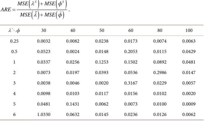
Properties and applications of the Neymann type A distribution have been studied by Johnson et al.[8] (p368-378). The mean and variance of X are given respectively by E X

( )

=

λ

ф and V X

( )

=

λ

ф

(

1+ф

)

. From these expressions,

moment estimators (MM) have closed form expressions, see section (4.1) for comparisons between MM estimators and SMHD estimators in a numerical study. For applications often the parameter λ_{is smaller than the parameter}

ф.

1.2.2. Esscher Transform Operator

(5)

trans-DOI: 10.4236/ojs.2018.81012 191 Open Journal of Statistics

form operator can be defined and, provided the tilting parameter τ introduced is identifiable, new distributions can be created from existing ones.

Let X be the original random variable with Laplace transform

κ

( )

s . The Esscher transform operator which can be viewed as a tilting operator is defined as

( )

s Esscher

( )

,

κ

(

s

_{( )}

τ

)

η

κ τ

+

= = _.

1.2.3. Shift Operator

Let

κ

( )

s be the Laplace transform of a positive continuous random variable X. The Laplace transform of Y =X−τ,Y≥ ≥τ 0 is given by eτ

κ

( )

s . So, we can define the shift operator as

( )

s Shift

( )

, eτ

( )

s

η

=

κ τ

=

κ

_.

In some cases, even the pmf of Y has a closed form but the maximum likelih-ood (ML) estimators might be attained at the boundaries, the ML estimators might not have the regular optimum properties.

Note that parallel to the closed form pgf expressions for these new discrete distributions, it is often simple to simulate from the new distributions if we can simulate from the original distribution before the operators are applied. For example, let us consider the new distribution obtained by using the Esscher op-erator. It suffices to simulate from the distribution before applying the operator and apply the acceptance-rejection method to obtain a sample from the Esscher transformed distribution. The situation is similar for new distributions created by the PM operator. If we can simulate one observation from the mixing distri-bution of Y which gives a realized value t and if it is not difficult to draw one observation from the distribution with LT

( )

t

s

κ then combining these two

(6)

ex-DOI: 10.4236/ojs.2018.81012 192 Open Journal of Statistics

pressible only using special functions such as the confluent hypergeometric functions. For these models, likelihood methods might also be difficult to im-plement.

This leads us to look for alternative methods such as the simulated minimum Hellinger distance (SMHD) methods for count data. We shall consider grouped count data and ungrouped count data. With grouped data, it leads to simulated chi-square type statistics which can be used for model testing for discrete or continuous models. These statistics are similar to the traditional Pearson statis-tics. For model testing with continuous distributions, continuous observations when grouped into intervals are reduced to count data and we do not need to integrate the model density functions on intervals using SMHD methods, it suf-fices to simulate from the continuous model and construct sample distribution functions to obtain estimate interval probabilities. Therefore, the scopes of ap-plications of simulated methods are widened due to these features.

We briefly describe the classical minimum Hellinger distance methods intro-duced by Simpson [14], Simpson [15] for estimation for count data in the next section and we shall develop inference methods based on a simulated version of this HD distance following Pakes and Pollard [16] (1989), who have developed an elegant asymptotic theory for estimators obtained by minimizing a simulated objective function expressible as the Euclidean norm of a random vector of functions. As an example, they have shown that the simulated minimum chi-square estimators without weight satisfy the regularity conditions for being consistent and have an asymptotic normal distribution, see Pakes and Pollard

[16] (p1048). They work with properties of some special classes of sets to check the regularity conditions of their Theorem 3.3. Meanwhile, Newey and McFad-den [17] (p2187) work with properties of random functions and introduce a stochastic version of the classical equicontinuity property of real analysis. In this paper, we shall also extend the notion of continuity of real analysis to a version which only holds in probability for random functions which we call continuity in probability for a sequence of random functions which is similar to the notion of continuity with probability one as discussed by Newey and McFadden [17]

(p2132) in their Theorem 2.6. We also use the property of the compact domains under considerations shrink as the sample size n→ ∞ to verify conditions of Theorem 3.3 given by Pakes and Pollard [16] (1989) for SMHD methods using

grouped data and conditions of Theorem 7.1 of Newey and McFadden [17]

(p2185) for ungrouped data. This approach appears to be new and simpler that other approaches which have been used in the literature to establish asymptotic normality for estimators using simulations; previous approaches are very general but they are also more complicated to apply. A similar notion of continuity in probability has been introduced in the literature of stochastic processes.

(7)

where the authors mention simulated methods of moments (MSM). The simu-lated version for HD methods will be referred to as version S and the original version which is deterministic will be referred to as version D in this paper. We briefly review the Hellinger distance and chi-square distance below and subse-quently develop simulated inference methods for grouped and ungrouped count data using HD distance.

1.3. Hellinger and Chi-Square Distance Estimation

Assume that we have a random sample of n independent and identically distri-buted

(iid) nonnegative observations X1,,Xn from a pmf pθ

( )

x with

0,1,

x=  and

(

θ1, ,θm

)

′

= 

θ

is the vector of parameters of interest, θ0 is the vector of the true parameters. If

the data are grouped into r= +k 1 disjoint intervals I_j,j=0,1,,k so that they form a partition of the nonnegative real line, the unweighted chi-square distance is defined to be

( )

(

( )

)

2 0

k

n j n j j

CS θ =

∑

₌ p I −p_θ I ,

where pn

( )

Ij is the proportion of the sample which fall into the interval Ij

and pθ

( )

Ij is the probability of an observation which fall into Ij under the

pmf p_θ

( )

x . If p_θ

( )

x has no closed form expression but we can draw a sam-ple of size U=τn from this distribution then clearly pθ

( )

Ij can be estimated

by S

( )

j

p_θ I using the simulated sample of size U which is the proportion of ob-servations of the simulated sample which has taken a value in Ij. To illustrate

their theory Pake and Pollard [16] (p1047-1048) considered simulated estima-tors obtained by minimizing with respect to θ _{the objective function}

( )

(

( )

)

2 0

k S

n j n j j

Q θ =

∑

₌ p I −pθ I

and show that the estimators satisfy the regularity conditions of their Theorem 3.1 and 3.3 which lead to conclude that the simulated estimators are consistent and have an asymptotic normal distribution. As we already know, a weighted version can be more efficient, if we attempt a version S for the Pearson’s chi square distance,

( )

(

( )

_{( )}

( )

)

2

0

n j j

k j

j

p I p I

P

p I

=

−

=

∑

θ

θ ,

and since the denominator of the summand involves pθ

( )

Ij , it is numerically

not easy to introduce a version S. Clearly, if S

( )

0

j

(8)

version of the Hellinger distance as given by

( )

2

1 1

2 2

0

k

n j n j j

Q = ₌ __p I _ −_p I _ _

 

∑

θ

θ (1)

is more appropriate for a version S and it is already known that it generates minimum HD estimators which are as efficient as the minimum chi-square es-timators or maximum likelihood (ML) eses-timators for grouped data, see

Cressie-Read divergence measure with 1

2

λ = − _{given by Cressie and Read}_[19]

(p457) for version D.

Note that

( )

1 1

2 2

0

HD θ = −2 2

∑

kj= pn Ij   pθ Ij  and by using Cauchy-

Schwartz inequality, we have

( )

1

( )

1

2 2

0

0≤

∑

kj= pn Ij   pθ Ij  ≤1,

so that 0≤Qn

( )

θ

≤2 and Qn

( )

θ

remains always bounded. Therefore the

objective function for version S can be defined as

( )

2

1 1

2 2

0

k S

n j n j j

Q = ₌ __p I _ −_p I _ _

 

∑

θ

θ _{. (2)}

Since the objective function remains bounded and this property continues to hold for the ungrouped data case, this suggests that SMHD methods could pre-serve some of the nice robustness properties of version D.

For ungrouped data, it is equivalent to have grouped data but using intervals with unit length Ij=

[

j j, +1 ,

)

j=0,1, and the number of classes is infinite,

we shall develop SMHD estimation which is based on the objective function

( )

2

1 1

2 2

0 2 2 0

S S

n j n i n

Q = ∞₌ _p j _ −_p j _  = − ∞₌ _p j _ _p j _

 

∑

θ

∑

θ

θ _{. (3)}

Note that for a data set the sum given by the RHS of the above expression only has a finite number of terms as pn

( )

j =0 when j is large.

The version D with

( )

12

( )

12 2

( )

12

( )

12

0 2 2 0

n j n i n

Q θ = ∞₌ __p j _ −_p j _ _ = − ∞₌ _p j _{ } p j _

 

∑

θ

∑

θ (4)

has been investigated by Simpson [14], Simpson [15] who also shows that the MHD estimators have a high breakdown point of at least 50% and first order as efficient as the ML estimators. For the Poisson case, the ML estimator is the sample mean which has a zero breakdown point and consequently far less robust than the HD estimators, yet the HD estimators are first order as efficient as the ML estimators. This feature makes HD estimators attractive. For the notion of finite sample break down point as a measure of robustness, see Hogg et al.[20]

(9)

breakdown point for large samples, see Maronna et al.[22] (p58).

Simpson [14], Simpson [15] extended the works of Beran [23] for continuous distributions to discrete distributions. Beran [23] appears to be the first to in-troduce a weaker form of robustness not based on bounded influence function and shows that efficiency can be achieved for robust estimators not based on in-fluence functions. Also, see Lindsay [24] for discussions on robustness of Hel-linger distance estimators. Simulated versions extending some of the seminal works of Simpson will be introduced in this paper.

SMHD methods appear to be useful for actuarial studies when there is a need for fitting discrete risk models, see chapter 9 of Panjer and Willmott [3]

(p292-238) for fitting discrete risk models using ML methods. The SMHD me-thods appear to be useful for other fields as well especially when there is a need to analyze count data with efficiency and robustness but the pmfs of the models do not have closed form expressions. For minimizing the objective functions to obtain SMHD estimators, simplex derivative free algorithm can be used and the R package already has built in functions to implement these minimization pro-cedures.

1.4. Outlines of the Paper

In this paper, we develop unified simulated methods of inferences for grouped and ungrouped count data using HD distances and it is organized as follows. Asymptotic properties for SMHD methods are developed in Section 2 where consistency and asymptotic normality are shown in Section 2.2. Based on asymptotic properties, consistency of the SMHD estimators hold in general but high efficiencies of SMHD estimators can only be guaranteed if the Fisher in-formation matrix of the parametric exists, a situation which is similar to likelih-ood estimation. One can also viewed the estimators are fully efficient within the class of simulated estimators obtained with the model pmf being replaced by a simulated version. Chi-square goodness of fit test statistics are constructed in Section 2.3. For the ungrouped case, it can be seen as having grouped data but the number of intervals with unit length and the number of intervals is infinite, it is given in Section 3 where the ungrouped SMHD estimators are shown to have good efficiencies. The breakdown point for the SMHD estimators remains at least 1

2 just as for the deterministic version. A limited simulation study is

(10)

ro-DOI: 10.4236/ojs.2018.81012 196 Open Journal of Statistics

bust than the ML estimator in the presence of outliers just as in the deterministic case as shown by Simpson [14] (p805). More works are needed in this direction in general and for assessing the performance SMHD estimators and comparisons with the performances of other traditional estimators in various parametric models in finite samples.

2. SMHD Methods for Grouped Data

2.1. Introduction

Pakes and Pollard [16] have developed a very elegant and general theory for es-tablishing consistency and asymptotic normality of estimators obtained by mi-nimizing the length of a random function taking values in an Euclidean space,

i.e., by minimizing

( )

n

G θ (5)

or

( )

(

)

2

n

G θ (6)

where n

( )

(

Gn,0

( )

, ,Gn k,

( )

)

′ =

G θ θ  θ is a vector of random functions with

values in a Euclidean space and ⋅ is the Euclidean norm and if

( )

a_ij ,i 1, , ,a j 1, ,b

= = =

A   is a matrix of finite dimension then

(

)

1

2

1 1

a b ij i= j=a

=

∑ ∑

A . Their theory is summarized by their Theorem 3.1 and

Theorem 3.3 given in Pakes and Pollard [16] (p1038-1043). It is very general and it is clearly applicable for both versions D and S for Hellinger distance with grouped data. Let

( )

(

( )

)

2

( )

(

( )

)

2

,

n n

Q θ = G θ Q θ = G θ (7)

and for HD distance, version D, let

( )

12

( )

12

( )

12

( )

12

0 0 , ,

n pn I p I pn Ik p Ik ′

 

       

=__ _ −_ _ _ _ −_ _ _

 

G θ _θ  _θ , (8)

and for version S, let

( )

12

( )

12

( )

12

( )

12

0 0 , ,

S S

n pn I p I pn Ik p Ik

′

 

   

=__ _ −_ _ _ _ −_ _ _

 

G θ _θ  _θ (9)

which can be reexpressed as

( )

1

1 1 1

2

2 2 2

0 0 0 0

1

1 1 1

2

2 2 2

, ,

S

n n

S

n k k k k

p I p I p I p I

θ θ θ

  _ _ 

     

=_  −  _{ }−  −    

′

 

  _ _

  −  − −  

         

   

G 

θ θ θ

θ

. (10)

In general, the intervals Ii’s form a partition of the nonnegative real line R0

(11)

with 0 0

k i i

R+=



₌ I . Only in section (2.3) where we want to test goodness of fit for continuous distribution with support of the entire real line used in financial

study, we might let 0

k i i

R=



₌ I , R is the real line.

Let

( )

0

( )

0

( )

1 1 1 1

2 2 2 2

0 0 , , k k

p I p I p I p I

′

 

       

=_ _ −_ _ _ _ −_ _ 

 

G θ _θ _θ  _θ _θ , the vector

of the true parameters is denoted by θ0∈Ω, the parameter space Ω is

as-sumed to be compact. Clearly, we have point wise convergence in probability

with

( )

p

( )

n

G

θ

→G

θ

for each θ for both versions, G

( )

θ is nonrandom. Clearly the set up fits into the scopes of their Theorem 3.1 and 3.3 which we shall rearrange the results of these two theorems before applying to version D and version S of Hellinger distance inferences and verify that we can satisfy the re-gularity conditions of these two Theorems.

2.2. Asymptotic Properties

2.2.1. Consistency

We define MHD estimators as given by the vector

θ

G for version D and  S G θ

for version S but emphasize version S as version D has been studied by Simpson

[14]. Both versions can be treated in a unified way using the following Theorem 1 for consistency which is essentially Theorem 3.1 of Pakes and Pollard [16]

(p1038) and the proof has been given by the authors. Theorem 1 (Consistency)

Under the following conditions θ_{converges in probability to}θ₀: a) Gn

( )

θ ≤op

( )

1 +infθ∈Ω

(

Gn

( )

θ

)

, the parameter space Ω is compact

b) Gn

( )

θ0 =op

( )

1 ,

c) sup ₀ 1

_{( )}

_p

( )

1

n

O δ

− >

 

=

 

 G 

θ θ _θ for each δ >0.

Theorem 3.1 states condition b) as Gn

( )

θ

0 =op

( )

1 but in the proof the

au-thors just use Gn

( )

θ0 =op

( )

1 so we state condition b) as Gn

( )

θ0 =op

( )

1 as

it is easier to use this condition when there is a need to extend to the infinite di-mensional case with the space 2

l .

An expression is op

( )

1 if it converges to 0 in probability and Op

( )

1 if it is

bounded in probability. In version D and version S for Hellinger distance we have infθ∈Ω

(

Gn

( )

θ

)

occurs at the values of the vector values of the HD

es-timators, so the conditions a) and b) are satisfied for both versions and com-pactness of the parameter space Ω is assumed. Also, for both versions

( )

p 0

n →

G θ only at θ θ= ₀ and 0<Q_n

( )

θ

≤2 otherwise, this implies

that there exist real numbers u and v with 0< < < ∞u v such that

( )

0

1

sup 1 as .

n

P u ₋ _>_δ v n

   

 ≤ _ _≤ → → ∞

 _ _ 

 θ θ G θ 

(12)

the minimum Hellinger distance estimators (MHD) are consistent. Theorem 3.1 of Pakes and Pollard [16] is an elegant theorem, its proof is also concise using the norm concept of functional analysis and it allows many results to be unified. Essentially, the same theorem remains valid with the use of the Hilbert space 2

l and its norm instead of the Euclidean space m

R and the Euclidean norm. By using 2

l and its norm the consistency for the ungrouped SMHD estimators can also be established but further asymptotic results for the ungrouped SMHD es-timators will be postponed and given in Section 3.

Asymptotic normality is more complicated in general. For the grouped case, Theorem 3.3 given by Pakes and Pollard [16] (p1040) can be used to establish asymptotic normality for both versions of Hellinger distance estimators. We shall rearrange results of Theorem 3.3 under Theorem 2 and Corollary 1 given in the next section to make it easier to apply for HD estimation using both ver-sions.

Since the proofs have been given by the authors, we only discuss here the ideas of their proofs to make it easier to follow the results of Theorem 2 and Corollary 1 in Section (2.2.2).

For both versions, Qn

( )

(

n

( )

)

2

(

n

( )

)

(

n

( )

)

′

= G = G G

θ

but Gn

( )

θ

is

not differentiable for version S, the traditional Taylor expansion argument can-not be used to establish asymptotic normality of estimators obtained by mini-mizing

(

( )

)

2

n

G θ . If we assume G

( )

θ is differentiable with derivative matrix

( )

θ

Γ _{, then we can define the random function} a

( )

n

Q

θ

to approximate Q_n

( )

θ

with

( )

(

( )

)

2

( )

( )(

)

0 0 0

,

a

n n n n

Q θ = L θ L θ =G θ +Γ θ θ − θ . (11)

( )

0

n

G

θ

is based on expression (8) for version D and it is based on

expres-sions (9-10) for version S. Note that a

( )

n

Q

θ

is differentiable for both ver-sions.

Let θ and _θ∗_{be the vectors which minimize}

( )

n

Q

θ

and Q_na

( )

θ

respec-tively. If the approximation is of the right order then θ_and _θ∗_are asymp-totically equivalent. This set up will allow a unified approach for establishing asymptotic for MHD estimation for both versions. For version D, it suffices to let

θ θ

=G and for version S, let 

S G

=

 θ θ .

Under these circumstances, it suffices to work with _θ∗_and a

( )

n

Q θ∗ for asymptotic properties of θ_and a

( )

n

Q θ∗ . A regularity condition for the ap-proximation is of the right order which implies the condition (iii) given by their Theorem 3.3, which is the most difficult to check is given as

( )

0 0

sup 1

n n n n op

δ

− ≤ G −G −G =

θ θ θ θ θ . (12)

This condition is used to formulate Theorem 2 below and is slightly more stringent than the condition iii) of their Theorem 3.3 but it is less technical and sufifcient for SMHD estimation. Clearly, for SMHD estimation Gn

( )

θ

is as

(13)

minimum chi-square estimation for this condition to hold, independent samples for each

θ

cannot be used, see Pakes and Pollard [16] (p1048). Otherwise, only consistency can be guaranteed for estimators using version S. For version S, the simulated samples are assumed to have size U=τn and the same seed is used across different values of

θ

to draw samples of size U. We implicitly make these assumptions for SMHD methods. These two assumption are standard for simulated methods of inferences, see section 9.6 for method of simulated mo-ments(MSM) given by Davidson and McKinnon [19] (p383-394). For numerical optimization to find the minimum of the objective function Qn

( )

θ

, we rely on

direct search simplex methods which are derivative free and the R package al-ready has prewritten functions to implement direct search methods.

2.2.2. Asymptotic Normality

In this section, we shall state a Theorem namely Theorem 2 which is essentially Theorem 3.3 by Pakes and Pollard [16] (p1040-1043) with the condition (4) of Theorem 2 given by expression (9) replacing their condition (iii) in their Theo-rem 3.3, the condition (4) implies the condition (iii) by being more stringent. We also comment on the conditions needed to verify asymptotic normality for the HD estimators based on Theorem 2.

Theorem 2

Let θ_{be a vector of consistent estimators for}θ₀_{, the unique vector which}

satisfies G

( )

θ

0 =0.

Under the following conditions:

1) The parameter space Ω is compact, θ is an interior point of Ω.

2)

( )

12 _inf

( )

n op n n

−

∈Ω

 

≤ _ _+

 



G θ _θ G θ .

3) G

( )

. is differentiable at θ0 with a derivative matrix Γ Γ=

( )

θ

0 of full

rank.

4) supθ θ−₀≤δ_n n Gn

( )

θ −G

( )

θ −Gn

( )

θ0 =op

( )

1 for every sequence

{ }

δn

of positive numbers which converge to zero. 5) Gn

( )

θ0 =op

( )

1 .

6) θ0 is an interior point of the parameter space Ω.

Then, we have the following representation which will give the asymptotic distribution of θ in Corollary 1, i.e.,

(

)

(

)

1

( )

0 n 0 p 1

n θ θ− = − Γ Γ′ − Γ′ nG θ +o , (13)

or equivalently, using equality in distribution,

(

)

(

)

1

( )

0 0

d

n

n θ θ− = − Γ Γ′ − nΓ′G θ . (14)

(14)

Theorem 2, it is easy to see that we can obtain the main result of the following Corollary 1 which gives the asymptotic covariance matrix for the HD estimators for both versions.

Corollary 1.

Let Yn = nΓ′Gn

( )

θ

0 , if

(

,

)

L n →N

Y 0V then n

(

θ θ− ₀

)

L→N

(

0,T

)

with

(

_′

)

−1

(

_′

)

−1 =

T Γ Γ V Γ Γ ,

The matrices T and V depend on θ0 we also adopt the notations

( )

0

=

T T

θ

, V =V

( )

θ

0 .

We observe that condition 4) of Theorem 2 when applies to Hellinger distance or in general involve technicalities. The condition 4) holds for version D, we on-ly need to verify for version S. Note that to verify the condition 4, it is equivalent to verify

( )

(

)

( )

0

2 0

sup 1

nn n n op

δ

− ≤ G −G −G =

θ θ θ θ θ

and for version S of Hellinger distance estimation, let

( )

(

( )

)

2 0

n n n

g θ =n G θ −G θ −G θ

and for the grouped case, it is given by

( )

₀

( )

₀

( )

2

1 1 1 1

2 2 2 2

0

k S S

n i j j j j

g =n ₌ ___p I _ −_p I _ _{ }  − _p I _ −_p I _ __

   

 

∑

θ θ θ θ

θ . (15)

We need to verify that we have the sequence of functions

{

gn

( )

θ

}

converge

uniformly to 0 in probability as n→ ∞ and θ →θ₀ or equivalently,

( )

0

sup 0

n

p n

g δ

− ≤ →

θ θ θ as n→ ∞ and θ→θ0.

Note that

( )

0 0

2 2

1 1 1 1

2 2 2 2

0

1 1 1 1

2 2 2 2

2 , 0.

k S S

n i j j j j

S S

j j j j n

g n p I p I p I p I

p I p I p I p I g

=

   

        

= __ _ −_ _ _ +__ _ −_ _ _

   





  

       

− __ _ −_ _ __ _ −_ _ _ ≥

  

∑

θ θ θ θ

θ

We shall outline the approach by first defining the notion of continuity in probability and let S

(

θ0,δn

)

=

{

θ θ θ− 0 ≤δn

}

which is a compact set. The

compactness of this set simplifies proofs and does not appear to be used in pre-vious approaches in the literature. Observe that gn

( )

θ

0 =0, it is easy to see that

( )

0 0

p

n n

g

θ

→g

θ

= as θ→θ₀. Subsequently we establish gn

( )

θ

being

continuous in probability for θ_{and using the property that}

{

g_n

( )

θ

}

is

con-tinuous in probability sup ₀

( )

ngn

δ − ≤

θ θ θ is attained at a point

0

=

θ θ _which

belongs to the compact set S

(

θ

0,

δ

n

)

in probability. This is similar to the

(15)

Now as n→ ∞,δn→0 which implies

0 0

→

θ

and by continuity in

proba-bility

( )

0

( )

0 0

p

n n n

g θ →g θ = . Therefore,

( )

0

sup 0

n

p n

g δ

− ≤ →

θ θ θ which

means that

{

gn

( )

θ

}

converges uniformly in probability as n→ ∞. The technical

details of these arguments are given in technical appendices TA1.1 and TA1.2 at the end of the paper, in the section of Appendices.

The notion of continuity in probability has been used in a similar context in the literature of stochastic processes, see Gusalk et al.[25] and will be introduced in the next paragraph and we also make a few assumptions which are summa-rized by Assumption 1 and Assumption 2 given below along with the notion of continuity in probability. A related continuity notion namely the notion of con-tinuity with probability one has been mentioned by Newey and McFadden [18]

in their Theorem 2.6 as mentioned earlier. They also commented that this no-tion can be used for establishing asymptotic properties of simulated estimators introduced by Pakes [26]. Pakes [26] also has used pseudo random numbers to estimate probability frequencies for some models. For SMHD estimation, we extend a standard result of analysis which states that a continuous function at-tains its supremum on a compact set to a version which holds in probability. This approach seems to be new and simpler than the use of the more general stochastic equicontinuity condition given by section 2.2 in Newey and McFadden [18] (p2136-2138) to establish uniform convergence of a sequence of random functions in probability. Our approach uses the fact that as n→ ∞ the set S

(

θ

0,

δ

n

)

shrinks to θ0, a property which did not seem to have been

used previously by other approaches to establish sup ₀

( )

0

n

p n

g δ

− ≤ →

θ θ θ as

n→ ∞ and θ→θ₀. Subsequently, we define the notion of continuity in probability which is similar to the one used in stochastic processes, see Gusak et al. [25] (p33) for a related notion of continuity in probability for stochastic processes.

Definition 1 (Continuity in probability)

A sequence of random functions

{

gn

( )

θ

}

is continuous in probability at θ′

if

( )

p

( )

n n

g

θ

→g

θ

′ whenever θ→θ′. Equivalently, for any >0,δ₁>0,

there exists a

δ

≥0 and n0 such that P g

(

n

( )

θ −gn

( )

θ′ ≤

)

≥ −1 δ1 for

0

n≥n , whenever

θ − θ

′ ≤

δ

. This can be viewed as an extension of the classical result of continuity in real analysis. It is also well known that the supremum of a continuous function on a compact domain is attained at a point of the compact domain, see Davidson and Donsig [27] (p81) or Rudin [28] (p89) for this clas-sical result. The equivalent property for a random function which is only conti-nuous in probability is the supremum of the random function is attained at a point of the compact domain in probability. The compact domain we study here is given by S

(

θ0,δn

)

=

{

θ θ θ− 0 ≤δn

}

and as n→ ∞, S

(

θ0,δ →n

)

θ0. It

(16)

ran-DOI: 10.4236/ojs.2018.81012 202 Open Journal of Statistics

dom function will depend on n.

Below are the assumptions we need to make to establish asymptotic normality for SMHD estimators and they appear to be reasonable.

Assumption 1

1) The pmf of the parametric model has the continuity property with

( )

1 1

2 2

pθ i →pθ′ i whenever θ →θ′.

2) The simulated counterpart has the continuity in probability property with _pS 12 p _pS 12

′

  → 

 θ  θ whenever θ →θ′. Convergence in probability is

denote by _→p _.

3) _p12

( )

_i

θ is differentiable with respect to θ.

In general, the condition 2) will be satisfied if the condition 1) holds and implicitly we assume the same seed is used for obtaining the simulated sam-ples across different values of θ_{. For ungrouped data, we also need the}

no-tion of differentiability in probability to facilitate the applicano-tion of Theorem 7.1 given by Newey and McFadden (1994, p2185-2186). Before stating their Theorem 7.1, Newey and McFadden has mentioned the notion of approx-imate derivative for the use of their Theorem, the definition given below will make it clearer.

Definition 2 (Differentiability in probability) The sequence of random functions

{ }

( )n

f_θ is differentiable with respect to θ

at θ0 in probability if

( ) ( )

( )

0 0

lim j

n n

e _p

j

f f

v

ε

+ →

− =

 

θ θ

θ , j=1,,m exists and

(

0, 0, ,1, 0, , 0

)

i

e =   ′ with 1 occurring at the ith entry. Furthermore, the vector

( )

(

1

( )

, , m

( )

)

v θ = v θ  v θ ′ is continuous and bounded in probability for all

(

0, 0

)

S

δ

∈

θ

for some δ >0 0. This concept is similar to the notion of

differentiability in real analysis for nonrandom function.

A similar notion of differentiability in probability has been used in stochastic processes literature, see Gusak et al.[25] (p33-34), a more stringent differentia-bility notion namely differentiadifferentia-bility in quadratic mean has also been used to study local asymptotic normality (LAN) property for a parametric family, see Keener [29] (p326). The notion of differentiability in probability will be used in section 3 with Theorem 7.1 of Newey and McFadden [17] to establish asymptot-ic normality for the SMHD estimators for the ungrouped case. We make the following assumption for _pS12

 θ where pθS can be viewed as a proxy model for p_θ,

Assumption 2

( )

12

S

p i

 

 θ  with the same seed being used across different values of θ is

dif-ferentiable in probability with the same derivative vector as _p12

( )

_i

(17)

derivative vector for _p12

( )

_i

θ is

( )

1 1

2 2

1

, ,

m

p i p i

sθ i _θ _θ

 

∂ ∂

 

=  _∂ _∂ 

 

 



θ θ _.

This assumption appears to be reasonable, this can be checked by using limit operations as in real analysis with _pS

( )

_i  →12 p _p12

( )

_i

 θ  θ and

( )

1 2

S

p i

 

 θ  is

continuous in probability.

Since regularity conditions for Theorem 2 and its corollary can be met and they are justified in TA1.1 and TA1.2 in the Appendices, we proceed here to find the asymptotic covariance matrix T.

Since Gn

( )

θ

0 for version D is based on expression (8) and for version S is

based on expressions (9-10), the asymptotic covariance matrix of nGn

( )

θ

0

version S is just the asymptotic covariance matrix of nGn

( )

θ

0 of version D

multiplied by 1 1

τ

 ₊ 

 

  as the simulated sample from pθ

( )

x is independent

from the sample given by the data, so we can focus on version D and make the adjustment for version S. We need the asymptotic covariance matrix Σ_{of the}

vector n n n p

(

n

( )

I0 , ,pn

( )

Ik

)

′ =

u  first then we can find the matrix T

and we let T=TD for version D and for version S, we shall let T =TS.

Recall that form properties of the multinomial distribution, the covariances of

( )

n i

n p I and n p_n

( )

I_j are

( )

(

_n _i , _n _j

)

(

₀

( )

_i

)

(

1 ₀

( )

_i

)

, for

nCov p I p I = p_θ I −p_θ I i= j

and

( )

(

_n _i , _n _j

)

(

₀

( )

_i

)

(

₀

( )

_j

)

, for .

nCov p I p I = − pθ I pθ I i≠ j

The covariance matrix of n n n p

(

n

( )

I0 , ,pn

( )

Ik

)

′ =

u  using matrix

nota-tions can be expressed as

(

)

1 1

2 2

− −

′ =Q I−qq Q

Σ , (16)

1 2

−

Q is a diagonal matrix with diagonal elements

( )

0 0

1 1

2 2

0 , , k

p I p I

′

 

   

_ _ _ _ 

 θ  θ  and the vector 0

( )

0

( )

1 1

2 2

0 , , k

p I p I

 

   

′ = _ _ _ _ 

 

q _θ  _θ

is the transpose of q and I is the identity matrix of dimension

r r

×

with

1

r= +k . Using the delta method the asymptotic covariance matrix of nG_n

( )

θ

₀ of version D is simply the asymptotic covariance matrix of

1 2

1

2Q nun which is

(18)

(

)

1 4

D = − ′

W I qq , (17)

and the asymptotic covariance matrix of nGn

( )

θ

0 , version S is

(

)

1 1 1 4 S   _′ = _ + _ −  

W I qq

τ

. (18)

We then have the vector of HD estimators version D and S given respectively by

θ

G and ˆ

S G

θ

with asymptotic distributions given by



(

0

)

(

,

)

,

L

D G

n θ −θ →N 0T

( )

1

(

) ( )

1

( )

1

( )

1 0 1 1 , 4 4 D G − − − − ′ ′ ′ ′ ′ = − = =

T Γ Γ Γ I qq Γ Γ Γ Γ Γ I θ (19)

( )

0 0 0 0 0 0 0 0 0 0 1 1 1 2 2 0 0 1 1 1 2 2 1 2 m k k m k k p I p I

p I p I

p I

p I p I

θ θ θ θ  ∂ ∂   _∂ _∂   _…        _ _ _ _    = −    _∂ _∂     ∂ ∂  …   _ _ _ _           θ θ θ θ θ θ θ θ Γ _,

( )

0

G

I

θ

is the model Fisher information matrix using grouped data as

′ =

qΓ 0 due to k_i₌₀∂p

( )

Ii =0

∂

∑

θ

using 0

( )

1

k i i= p I =

∑

θ . Let B= −2Γ,

( )

0 0 0 0 0 0 0 0 0 0 1 1 1 2 2 0 0 1 1 1 2 2 m k k m k k p I p I

p I p I

p I

p I p I

θ θ θ θ  ∂ ∂   _∂ _∂   _…        _ _ _ _    =    _∂ _∂     ∂ ∂  …   _ _ _ _       

B   

θ θ θ θ θ θ θ θ , so

(

)

1

D

−

′ =

T B B

with

( )

0 0 0 0 1 2 1 2 log

, 0,1, , , 1, ,

i i j i j i p I p I

p I i k j m

p I θ θ ∂ ∂ ∂   =_ _ = = ∂       θ θ θ θ .

Therefore for version S,

(

)

(

)

(

)

1

0

1

ˆS L _0, _, ₁

G S S

n N

τ

−  _{ ′} − → = +_ _  

T T B B

(19)

the simulated sample size is U=nτ.

Note that for version D, the HD estimators are as efficient as the minimum chi-square estimators or ML estimators based on grouped data. The overall asymptotic relative efficiency (ARE) between version D and S for HD estimation is simply ARE =

1

τ

τ+ and we recommend to set τ ≥10 to minimize the loss of

efficiency due to simulations.

An estimate for the covariance matrix The asymptotic covariance matrix of S G

θ _{can be estimated if we can estimate}

( )

0

=

θ

Γ Γ . Using a result given by Pakes and Pollard (1989, p1043), an estimate for Γ is the matrix



(

)

( )



(



)

( )



1

ˆ _, _,

S S S S

n G n n G n G n m n G n

n n

G e G G e G

 ₊ ₋ ₊ ₋ 

 

=  

 

 



 

θ θ θ θ

Γ _{, (21)}

(

0, 0, ,1, 0, , 0

)

i

e =   ′ with 1 occurring at the ith entry of the vector

, 1, ,

i

e i=  m and n n

δ −

=

 , 1

2

δ ≤ _{and in general we can let} 1

2

δ = _{. Note that}

the columns of ˆ

n

Γ _{estimate the corresponding partial derivatives given by the}

columns of Γ.

For ungrouped data and for version D, it is equivalent to choose Ij=

[

j j, +1

)

with unit length and let k= ∞. If we choose Ij=

[

j j, +1

)

and let k→ ∞ and

note that

(

B B′

)

→I

( )

θ

0 and I

( )

θ

0 the is Fisher information matrix for

un-grouped data with elements given by

( )

, 0

log log

, 1, , , 1, ,

h l i

h l

p i p i

I p i l m h m

θ θ

∞ =

∂ ∂

 

= _ _ = =

∂ ∂

 

∑

θ θ θ   (22)

and pθ

( )

i =pθ

( )

Ii ,Ii=

[

i i, +1 ,

)

θ θ

= 0. We can foresee that the HD estimators

are as efficient as ML estimators for version D, a result which is already obtained by Simpson [14]. We postpone till section (3) for a more rigorous approach to justify the related result for version S using Theorem 7.1 given by Newey and McFadden [17]. The SMHD estimators given by

θ

S _{for ungrouped data will be}

shown to have the property



(

)

(

( )

)

1

0 0

1 0, 1

L S

n N

τ

−

   

− → _ _ + _ _

 

 I 

θ θ θ .

Section 3 may be skipped for practitioners if their main interests are only on applications of the results.

2.3. Chi-Square Goodness of Fit Test Statistics

2.3.1. Simple Hypothesis

In this section, the Hellinger distance Qn

( )

θ

is used to construct goodness of

fit test statistics for the simple hypothesis

(20)

be the distribution of a discrete or continuous distribution. The chi-square test statistics and their asymptotic distributions are given below with

( )

2

(

)

0

4nQ_n θ L→χ r= k+ −1 1 for version andD (23)

( )

2

(

)

0 for v

4 1 1

1 ersion .

L n

n

τ

Q

χ

r k S

τ

  __→ ₌ _{+ −}

 ₊ 

 

θ

(24)

The version S is of interest since it allows testing goodness of fit for discrete or continuous distribution without closed form pmfs or density functions, all we need is to be able to simulate from the specified distribution. We shall justify the asymptotic chi-square distributions given by expression (23) and expression (24) below.

Note that

( )

0

( )

0

( )

0

4nQ_n

θ

= nG_n′

θ

nG_n

θ

and

( )

0

(

)

1 0,

4

L n

n →N_ − ′ _

 

G

θ

I qq

for version D. For version S,

( )

0

(

)

1 1

0, 1

4

L n

n N

τ

   _′ 

→ _ _ + _ − _

 

G θ I qq .

Using standard results for distribution of quadratic forms and the property of the operator trace of a matrix with

(

)

( )

( ) (

1

)

1

trace I−qq′ =trace I −trace qq′ = k+ − =k, see Luong and Thompson

[30] (p247); we have the asymptotic chi-square distributions as given by expres-sion (23) and expresexpres-sion (24). On how to choose the intervals, the problem is rather complex as it depends on the type of alternatives we would like to detect. We can also follow the recommendations of the Pearson’s statistics, see Green-wood and Nikulin [31]; also see Lehmann [32] (p341) for more discussions and references on this issue.

2.3.2. Composite Hypothesis

Just as the chi-square distance, the Hellinger distance Qn

( )

θ

can also be used

for construction of the test statistics for the composite hypothesis,

H0: data comes from a parametric model

{ }

Fθ ,

{ }

Fθ can be a discrete or continuous parametric model. The chi-square test statistics are given by



( )

2

(

)

4nQn θG →L χ r= −k m , (25)

for version D and for version S,



( )

2

(

)

4 1

L S n G

n

τ

Q

χ

r k m

τ

  _→ _{= −}

 ₊ 

 

θ

(26)

where

θ

G and  S G

θ are the vector of HD estimators which minimize Qn

( )

θ