Sequential decision problems, dependent types and generic solutions

SEQUENTIAL DECISION PROBLEMS, DEPENDENT TYPES AND GENERIC SOLUTIONS

NICOLA BOTTAa, PATRIK JANSSONb, CEZAR IONESCUc, DAVID R. CHRISTIANSENd, AND EDWIN BRADYe

a

Potsdam Institute for Climate Impact Research (PIK), Germany e-mail address: botta@pik-potsdam.de

b,c

Chalmers University of Technology & University of Gothenburg, Sweden e-mail address: {patrikj, cezar}@chalmers.se

d _{Indiana University, USA}

e-mail address: davidchr@indiana.edu

e

University of St Andrews, Scotland e-mail address: ecb10@st-andrews.ac.uk

Abstract. We present a computer-checked generic implementation for solving finite-horizon sequential decision problems. This is a wide class of problems, including inter-temporal optimizations, knapsack, optimal bracketing, scheduling, etc. The implementation can handle time-step dependent control and state spaces, and monadic representations of uncertainty (such as stochastic, non-deterministic, fuzzy, or combinations thereof). This level of genericity is achievable in a programming language with dependent types (we have used both Idris and Agda). Dependent types are also the means that allow us to obtain a formalization and computer-checked proof of the central component of our implementation: Bellman’s principle of optimality and the associated backwards induction algorithm. The formalization clarifies certain aspects of backwards induction and, by making explicit notions such as viability and reachability, can serve as a starting point for a theory of controllability of monadic dynamical systems, commonly encountered in, e.g., climate impact research.

b,c_{Jansson and Ionescu were supported by the projects GRACeFUL (grant agreement No 640954) and}

CoeGSS (grant agreement No 676547), which have received funding from the European Unions Horizon 2020 research and innovation programme.

d

Christiansen was funded by the Danish Advanced Technology Foundation (Hjteknologifonden) grant 17-2010-3.

LOGICAL METHODS

l

c

N. Botta, P. Jansson, C. Ionescu, D. R. Christiansen, and E. Brady

CC

1. Introduction

In this paper we extend a previous formalization oftime-independent,deterministicsequential decision problems [BIB13] to general sequential decision problems (general SDPs).

Sequential decision problems are problems in which a decision maker is required to make a step-by-step sequence of decisions. At each step, the decision maker selects a control upon observing somestate.

Time-independent, deterministic SDPs are sequential decision problems in which the state space (the set of states that can be observed by the decision maker) and the control space (the set of controls that can be selected in a given state) do not depend on the specific decision step and the result of selecting a control in a given state is a unique new state.

In contrast, general SDPs are sequential decision problems in which both the state space and the control space can depend on the specific decision step and the outcome of a step can be a set of new states (non-deterministic SDPs), a probability distribution of new states (stochastic SDPs) or, more generally, a monadic structure of states, see section 2.

Throughout the paper, we use the word “time” (and correspondent phrasings: “time-independent”, “time-dependent”, etc.) to denote a decision step number. In other words, we write “at time 3 . . . ” as a shortcut for “at the third decision step . . . ”. The intuition is that decision step 3 takes place after decision steps 0, 1 and 2 and before decision steps 4, 5, etc. In certain decision problems, some physical time – discrete or, perhaps, continuous – might be observable and relevant for decision making. In these cases, such time becomes a proper component of the state space and the function that computes a new state from a current state and a control has to fulfill certain monotonicity conditions.

Sequential decision problems for a finite number of steps, often called finite horizon SDPs, are in principle well understood. In standard textbooks [CSRL01, Ber95, SG98], SDPs are typically introduced by examples: a few specific problems are analyzed and dissected and ad-hoc implementations of Bellman’s backwards induction algorithm [Bel57] are derived for such problems.

To the best of our knowledge, no generic algorithm for solving general sequential decision problems is currently available. This has a number of disadvantages:

An obvious one is that, in front of a particular instance of an SDP, be that a variant of knapsack, optimal bracketing, inter-temporal optimization of social welfare functions or more specific applications, scientists have to find solution algorithms developed for similar problems — backwards induction or non-linear optimization, for example — and adapt or re-implement them for their particular problem.

This is not only time-consuming but also error-prone. For most practitioners, showing that their ad-hoc implementation actually delivers optimal solutions is often an insurmount-able task.

In this work, we address this problem by using dependent types — types that are allowed to “depend” on values [Bra13] — in order to formalise general SDPs, implement a generic version of Bellman’s backwards induction, and obtain a machine-checkable proof that the implementation is correct.

concrete program and a concrete proof of correctness. An error in the instantiation will result in an error in the proof, and will be signalled by the type checker.

Expert implementors might want to re-implement problem-specific solution algorithms, e.g., in order to exploit some known properties of the particular problem at hand. But they would at least be able to test their solutions against provably correct ones. Moreover, if they use the framework, the proof obligations are going to be signalled by the type checker.

The fact that the specifications, implementations, and proof of correctness are all expressed in the same programming language is, in our opinion, the most important advantage of dependently-typed languages. Any change in the implementation immediately leads to a verification against the specification and the proof. If something is wrong, the implementation is not executed: the program does not compile. This is not the case with pencil-and-paper proofs of correctness, or with programs extracted from specifications and proofs using a system such as Coq.

Our approach is similar in spirit to that proposed by de Moor [dM95] and developed in theAlgebra of Programming book [BdM97]. There, the specification, implementation, and proof are all expressed in the relational calculus of allegories, but they are left at the paper and pencil stage. For a discussion of other differences and of the similarities we refer the reader to our previous paper [BIB13], which the present paper extends.

This extension is presented in two steps. First, we generalize time-independent (remember that we use the word “time” as an alias to “decision step”; thus, time-independent SDPs are sequential decision problems in which the state space and the control space do not depend on the decision step), deterministic decision problems to the case in which the state and the control spaces can depend on time but the transition function is still deterministic. Then, we extend this case to the general one of monadic transition functions. As it turns out, neither extension is trivial: the requirement of machine-checkable correctness brings to the light notions and assumptions which, in informal and semi-formal derivations are often swept under the rug.

In particular, the extension to the time-dependent case has lead us to formalize the notions of viability andreachability of states. For the deterministic case these notions are more or less straightforward. But they become more interesting when non-deterministic and stochastic transition functions are considered (as outlined in section 5).

We believe that these notions would be a good starting point for building a theory of controllability for the kind of dynamical systems commonly encountered in climate impact research. These were the systems originally studied in Ionescu’s dissertation [Ion09] and the monadic case is an extension of the theory presented there for dynamical systems.

In the next section we introduce, informally, the notion of sequential decision processes and problems. In section 3 we summarize the results for the time-independent, deterministic case and use this as the starting point for the two extensions discussed in sections 4 and 5, respectively.

2. Sequential decision processes and problems

In a nutshell, a sequential decision process is a process in which a decision maker is required to take a finite number of decision steps, one after the other. The process starts in a state x0 at an initial step numbert0.

Herex0 represents all information available to the decision maker att0. In a decision

x0 could be a triple of real numbers representing some estimate of the greenhouse gas (GHG)

concentration in the atmosphere, a measure of a gross domestic product and, perhaps, the number of years elapsed from some pre-industrial reference state. In an optimal bracketing problem,x0 could be a string of characters representing the “sizes” of a list of “arguments”

which are to be processed pairwise with some associative binary operation. In all cases,t0 is

the initial value of the decision step counter.

The control space – the set of controls (actions, options, choices, etc.) available to the decision maker – can depend both on the initial step number and state. Upon selecting a control y0 two events take place: the system enters a new statex1 and the decision maker

receives a reward r0.

In a deterministic decision problem, a transition function completely determines the next state x1 given the time (step number) of the decision t0, the current state x0, and

the selected controly0. But, in general, transition functions can return sets of new states

(non-deterministic SDPs), probability distributions over new states (stochastic SDPs) or, more generally, a monadic structures of states, as presented by Ionescu [Ion09].

In general, the reward depends both on the “old” state and on the “new” state, and on the selected control: in many decision problems, different controls represent different levels of consumption of resources (fuel, money, CPU time or memory) or different levels of restrictions (GHG emission abatements) and are often associated with costs. Different current and next states often imply different levels of “running” costs or benefits (of machinery, avoided climate damages, . . . ) or outcome payoffs.

The intuition of finite horizon SDPs is that the decision maker seeks controls that maximize the sum of the rewards collected over a finite number of decision steps. This characterization of SDPs might appear too narrow (why shouldn’t a decision maker be interested, for instance, in maximizing a product of rewards?) but it is in fact quite general. For an introduction to SDPs and concrete examples of state spaces, control spaces, transition-and reward-functions, see [Ber95, SG98].

In control theory, controls that maximize the sum of the rewards collected over a finite number of steps are called optimal controls. In practice, optimal controls can only be computed when a specific initial state is given and for problems in which transitions are deterministic. What is relevant for decision making – both in the deterministic case and in the non-deterministic or stochastic case – are not controls butpolicies.

Informally, a policy is a function from states to controls: it tells which control to select when in a given state. Thus, for selecting controls over n steps, a decision maker needs a sequence ofn policies, one for each step. Optimal policy sequences are sequences of policies which cannot be improved by associating different controls to current and future states.

3. Time-independent, deterministic problems

In a previous paper [BIB13], we presented a formalization of time-independent, deterministic SDPs. For this class of problems, we introduced an abstract context and derived a generic, machine-checkable implementation of backwards induction.

a b c d e 0 1 2 3 4 5 6 7 ... ... n

a b c d e 0 1 2 3 4 5 6 7 ... ... n 3 ?

a b c d e 0 1 2 3 4 5 6 7 ... ... n 3 5 4 4 ?

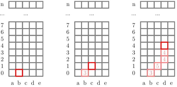
Figure 1: Possible evolutions for the “cylinder” problem. Initial state (b, left), state and reward after one step (cand 3, middle) and four steps trajectory and rewards (right).

A decision-maker can be in one of five states: a,b,c,d ore. Ina, the decision maker can choose between two controls (sometimes called “options” or “actions”): move ahead (control A) or move to the right (control R). In b, c and d he can move to the left (L),

ahead or to the right. In e he can move to the left or go ahead.

Upon selecting a control, the decision maker enters a new state. For instance, selecting R inb brings him fromb to c, see Figure 1. Thus, each step is characterized by a current state, a selected control and a new state. A step also yields a reward, for instance 3 for the transition fromb toc and for control R.

The challenge for the decision maker is to make a finite number of steps, say n, by selecting controls that maximize the sum of the rewards collected.

An example of a possible trajectory and corresponding rewards for the first four steps is shown on the right of figure 1. In this example, the decision maker has so far collected a total reward of 16 by selecting controls according to the sequence [R,R,A,A]: R in the first and in the second steps, Ain the third and in the fourth steps.

In this problem, the set of possible statesState={a, b, c, d, e} is constant for all steps and the controls available in a state only depend on that state. The problem is an instance of a particular class of problems called time-independent, deterministic SDPs. In our previous paper [BIB13] we characterized this class in terms of four assumptions:

(1) The state space does not depend on the current number of steps.

(2) The control space in a given state only depends on that state but not on the current number of steps.

(3) At each step, the new state depends on the current state and on the selected control via a known deterministic function.

(4) At each step, the reward is a known function of the current state, of the selected control and of the new state.

and controls.) The results obtained [BIB13] for this class of sequential decision problems can be summarized as follows: The problems can be formalized in terms of a context containing states Stateand controlsCtrl from each state:

State : Type

Ctrl : (x : State) → Type

step : (x : State) → (y : Ctrl x) → State

reward : (x : State) → (y : Ctrl x) → (x0 : State) → _R

and of the notions of control sequence CtrlSeq x n (from a starting state x : State and for n : N steps), value of control sequences and optimality of control sequences:

dataCtrlSeq : State → _N → Type where Nil : CtrlSeq x Z

(::) : (y : Ctrl x) → CtrlSeq (step x y)n → CtrlSeq x (S n)

value : CtrlSeq x n → R

value {n =Z} = 0

value {x} {n =S m}(y::ys) =reward x y (step x y) +value ys

OptCtrlSeq : CtrlSeq x n → Type

OptCtrlSeq {x} {n}ys= (ys0 : CtrlSeq x n) → So(value ys0 6value ys)

In the above formulation, CtrlSeq x n formalizes the notion of a sequence of controls of length n with the first control in Ctrl x. In other words, if we are givenys : CtrlSeq x n and we are inx, we know that we can select the first control of ys.

The function value computes the value of a control sequence. As explained in the beginning of this section, the challenge for the decision maker is to select controls that maximize a sum of rewards. Throughout this paper, we use + to compute the sum. But it is clear that + does not need to denote standard addition. For instance, the sum could be “discounted” through lower weights for future rewards.

Thus, a sequence of controls ps : CtrlSeq x n is optimal iff any other sequence ps0 : CtrlSeq x n has a value that is smaller or equal to the value of ps. The value of a control sequence of length zero is zero and the value of a control sequence of length S m is computed by adding the reward obtained with the first decision step to the value of making m more decisions with the tail of that sequence.

In the above, the argumentsx and n toCtrlSeq in the types ofvalue and OptCtrlSeq

occur free. In Idris (as in Haskell), this means that they will be automatically inserted as implicit arguments. In the definitions of value and OptCtrlSeq, these implicit arguments are brought into the local scope by adding them to the pattern match surrounded by curly braces. We also use the functionSo : Bool → Type for translating between Booleans and types (the only constructor is Oh : So True).

We have shown that one can compute optimal control sequences from optimal policy sequences. These are policy vectors that maximize the value functionval for every state:

Policy : Type

Policy = (x : State) → Ctrl x

PolicySeq : N → Type

val : (x : State) → PolicySeq n → _R

val {n =Z} = 0

val {n =S m}x (p::ps) =reward x (p x)x0+val x0ps where x0 : State

x0 =step x (p x)

OptPolicySeq : (n : N) → PolicySeq n → Type

OptPolicySeq n ps = (x : State) → (ps0 : PolicySeq n) → So(val x ps0 6val x ps) We have expressed Bellman’s principle of optimality [Bel57] in terms of the notion of optimal extensions of policy sequences

OptExt : PolicySeq n → Policy → Type

OptExt ps p = (p0 : Policy) → (x : State) → So(val x (p0::ps)6val x (p::ps)) Bellman : (ps : PolicySeq n) → OptPolicySeq n ps →

(p : Policy) → OptExt ps p →

OptPolicySeq (S n) (p::ps)

and implemented a machine-checkable proof of Bellman. Another machine-checkable proof guarantees that, if one can implement a functionoptExt that computes an optimal extension of arbitrary policy sequences

OptExtLemma : (ps : PolicySeq n) → OptExt ps(optExt ps)

then

backwardsInduction : (n : N) → PolicySeq n

backwardsInduction Z = Nil

backwardsInduction (S n) = (optExt ps) ::ps where ps : PolicySeq n

ps =backwardsInduction n

yields optimal policy sequences (and, thus, optimal control sequences) of arbitrary length:

BackwardsInductionLemma : (n : N) → OptPolicySeq n (backwardsInduction n)

In our previous paper [BIB13], we have shown that it is easy to implement a function that computes the optimal extension of an arbitrary policy sequence if one can implement

max : (x : State) → (Ctrl x → _R) → _R

argmax : (x : State) → (Ctrl x → R) → Ctrl x

which fulfill the specifications

MaxSpec : Type

MaxSpec = (x : State) → (f : Ctrl x → _R) → (y : Ctrl x) →

So(f y 6max x f) ArgmaxSpec : Type

ArgmaxSpec= (x : State) → (f : Ctrl x → _R) →

So(f (argmax x f) ==max x f)

4. Time-dependent state spaces

The results summarized in the previous section are valid under one implicit assumption: that one can construct control sequences of arbitrary length from arbitrary initial states. A sufficient (but not necessary) condition for this is that, for allx : State, the control space Ctrl x is not empty. As we shall see in a moment, this assumption is too strong and needs

to be refined.

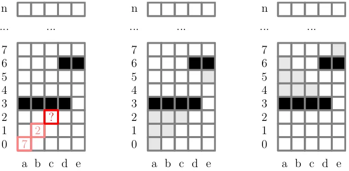
Consider, again, the cylinder problem. Assume that at a given decision step, only certain columns arevalid. For instance, fort 6= 3 and t 6= 6 all states a throughe are valid but at step 3 only e is valid and at step 6 only a,b andc are valid, see figure 2. Similarly, allow the controls available in a given state to depend both on that state and on the decision step. For instance, from state b at step 0 one might be able to move ahead or to the right. But at step 6 and from the same state, one might only be able to move to the left.

Note that a discrete time (number of decision steps) could be accounted for in different ways. One could for instance formalize “time-dependent” states as pairs (N,Type) or, as

we do, by adding an extra N argument. A study of alternative formalizations of general

decision problems is a very interesting topic but goes well beyond the scope of this work. We can provide two “justifications” for the formalization proposed here: that this is (again, to the best of our knowledge) the first attempt at formalizing such problems generically and that the formalization via additionalN arguments seems natural if one considers how

(non-autonomous) dynamical systems are usually formalized in the continuous case through systems of differential equations.

We can easily formalize the context for the time-dependent case by adding an extraN

argument to the declarations of State andCtrl and extending the transition and the reward functions accordingly (whereS : N → N is the successor function).

State : (t : N) → Type

Ctrl : (t : N) → State t → Type

step : (t : N) → (x : State t) → Ctrl t x → State (S t)

reward : (t : N) → (x : State t) → Ctrl t x → State (S t) → R

In general we will be able to construct control sequences of a given length from a given initial state only ifState,Ctrl andstep satisfy certain compatibility conditions. For example, assuming that the decision maker can move to the left, go ahead or move to the right as described in the previous section, there will be no sequence of more than two controls starting froma, see figure 2 left. At stept, there might be states which are valid but from which only m<n −t steps can be done, see figure 2 middle. Conversely, there might be states which are valid but which cannot be reached from any initial state, see figure 2 right.

We use the termviability to refer to the conditions that State,Ctrl andstep have to satisfy for a sequence of controls of lengthn starting inx : State t to exist. More formally, we say that every state is viable for zero steps (viableSpec0) and that a state x : State t is viable forS n steps if and only if there exists a command in Ctrl t x which, viastep, brings x into a state which is viablen steps (viableSpec1 and viableSpec2):

viable : (n : N) → State t → Bool

viableSpec0 : (x : State t) → Viable Z x

viableSpec1 : (x : State t) → Viable (S n)x → GoodCtrl t n x viableSpec2 : (x : State t) → GoodCtrl t n x → Viable (S n)x

In the above specifications we have introducedViable n x as a shorthand forSo(viable n x). InviableSpec1 andviableSpec2 we use subsets implemented as dependent pairs:

GoodCtrl : (t : N) → (n : N) → State t → Type

GoodCtrl t n x = (y : Ctrl t x ∗∗Viable n (step t x y))

These are pairs in which the type of the second element can depend on the value of the first one. The notation p : (a : A ∗∗P a) represents a pair in which the type (P a) of the second element can refer to the value (a) of the first element, giving a kind of existential quantification [Bra13]. The projection functions are

outl : {A : Type} → {P : A → Type} → (a : A ∗∗P a) → A

outr : {A : Type} → {P : A → Type} → (p : (a : A ∗∗P a)) → P (outl p)

Thus, in general (a : A ∗∗P a) effectively represents the subset of Awhose elements fulfill P and our case GoodCtrl t n x is the subset of controls available inx at stept which lead to next states which are viablen steps.

The declarations ofviableSpec0,viableSpec1 andviableSpec2 are added to the context. In implementing an instance of a specific sequential decision problem, clients are required to defineState,Ctrl, step, reward and the viable predicate for that problem. In doing so, they have to prove (or postulate) that their definitions satisfy the above specifications.

a b c d e 0

1 2 3 4 5 6 7

... ...

n

7 2

?

a b c d e 0

1 2 3 4 5 6 7

... ...

n

a b c d e 0

1 2 3 4 5 6 7

... ...

n

4.2. Control sequences. With the notion of viability in place, we can readily extend the notion of control sequences of section 3 to the time-dependent case:

dataCtrlSeq : (x : State t) → (n : N) → Type where

Nil : CtrlSeq x Z

(::) : (yv : GoodCtrl t n x) → CtrlSeq(step t x (outl yv))n → CtrlSeq x (S n)

Notice that now the constructor :: (for constructing control sequences of lengthS n) can only be applied to those (implicit !) x : State t for which there exists a “good” control y =outl yv : Ctrl t x such that the new statestep t x y is viablen steps. The specification viableSpec2 ensures us that, in this case, x is viableS n steps.

The extension of val, OptCtrlSeq and the proof of optimality of empty sequences of controls are, as one would expect, straightforward:

val : (x : State t) → (n : N) → CtrlSeq x n → R

val Z = 0

val {t}x (S n) (yv ::ys) =reward t x y x0+val x0n ys where y : Ctrl t x; y =outl yv

x0 : State (S t); x0 =step t x y

OptCtrlSeq : (x : State t) → (n : N) → CtrlSeq x n → Type

OptCtrlSeq x n ys = (ys0 : CtrlSeq x n) → So(val x n ys06val x n ys) nilIsOptCtrlSeq : (x : State t) → OptCtrlSeq x Z Nil

nilIsOptCtrlSeq x Nil =reflexive Double lte0

4.3. Reachability, policy sequences. In the time-independent case, policies are functions of type (x : State) → Ctrl x and policy sequences are vectors of elements of that type. Given a policy sequence ps and an initial state x, one can construct its corresponding sequence of controls by ctrls x ps:

ctrl : (x : State) → PolicySeq n → CtrlSeq x n ctrl x Nil =Nil

ctrl x (p::ps) =p x ::ctrl (step x (p x))ps

Thus p x is of typeCtrl x which is, in turn, the type of the first (explicit) argument of the “cons” constructor ofCtrlSeq x n, see section 3.

As seen above, in the time-dependent case the “cons” constructor ofCtrlSeq x n takes as first argument dependent pairs of type GoodCtrl t n x. For sequences of controls to be construable from policy sequences, policies have to return, in the time-dependent case, values of this type. Thus, what we want to formalize in the time-dependent case is the notion of a correspondence between states and sets of controls that, at a given stept, allows us to make a given number of decision steps n. Because of viableSpec1 we know that such controls exist for a given x : State t if and only if it is viable at leastn steps. We use such a requirement to restrict the domain of policies

Policy : N → N → Type

Policy t Z =Unit

Here,Unit is the singleton type. It is inhabited by a single value called (). Logically,Policy states that policies that supports zero decision steps are trivial values. Policies that support S n decision steps starting from states at timet, however, are functions that map states at time t which are reachable and viable forS n steps to controls leading to states (at time S t) which are viable for n steps.

Let us go back to the right-hand side of figure 2. At a given step, there might be states which are valid but which cannot be reached. It could be a waste of computational resources to consider such states, e.g., when constructing optimal extensions inside a backwards induction step.

We can compute optimal policy sequences more efficiently if we restrict the domain of our policies to those states which can actually be reached from the initial states. We can do this by introducing the notion ofreachability. We say that every initial state is reachable (reachableSpec0) and that if a state x : State t is reachable, then every controly : Ctrl t x

leads, viastep, to a reachable state inState (S t) (seereachableSpec1). Conversely, if a state x0 : State (S t) is reachable then there exist a state x : State t and a control y : Ctrl t x such thatx is reachable and x0 is equal to step t x y (see reachableSpec2):

reachable : State t → Bool

reachableSpec0 : (x : State Z) → Reachable x

reachableSpec1 : (x : State t) → Reachable x → (y : Ctrl t x) →

Reachable (step t x y)

reachableSpec2 : (x0 : State (S t)) → Reachable x0 →

(x : State t ∗∗(Reachable x,(y : Ctrl t x ∗∗x0 =step t x y)))

As for viability, we have introduced Reachable x as a shorthand for So(reachable x) in the specification of reachable. We can now apply reachability to refine the notion of policy

Policy : N → N → Type

Policy t Z =Unit

Policy t (S n) = (x : State t) → Reachable x → Viable (S n)x → GoodCtrl t n x

and policy sequences:

dataPolicySeq : N → N → Type where

Nil : PolicySeq t Z

(::) : Policy t(S n) → PolicySeq(S t)n → PolicySeq t (S n)

In contrast to the time-independent case, PolicySeq now takes an additionalNargument.

This represents the time (number of decision steps, value of the decision steps counter) at which the first policy of the sequence can be applied. The previous one-index idiom

(S n) · · · n · · · (S n) becomes a two-index idiom: t (S n) · · · (S t) n · · · t (S n). The

value functionval maximized by optimal policy sequences is:

val : (t : N) → (n : N) →

(x : State t) → (r : Reachable x) → (v : Viable n x) →

PolicySeq t n → R

val Z = 0

val t (S n)x r v (p::ps) =reward t x y x0+val (S t)n x0 r0v0ps where y : Ctrl t x; y =outl (p x r v)

r0 : Reachable x0; r0 =reachableSpec1 x r y v0 : Viable n x0; v0 =outr (p x r v)

4.4. The full framework. With these notions of viability, control sequence, reachability, policy and policy sequence, the previous [BIB13] formal framework for time-independent sequential decision problems can be easily extended to the time-dependent case.

The notions of optimality of policy sequences, optimal extension of policy sequences, Bellman’s principle of optimality, the generic implementation of backwards induction and its machine-checkable correctness can all be derived almost automatically from the time-independent case.

We do not present the complete framework here (but it is available on GitHub). To give an idea of the differences between the time-dependent and the time-independent cases, we compare the proofs of Bellman’s principle of optimality.

Consider, first, the time-independent case. As explained in section 3, Bellman’s principle of optimality says that if ps is an optimal policy sequence of lengthn andp is an optimal extension ofps thenp::ps is an optimal policy sequence of lengthS n. In the time-dependent case we need as additional argument the current number of decision stepst and we make the length of the policy sequencen explicit. The other arguments are, as in the time-independent case, a policy sequenceps, a proof of optimality ofps, a policy p and a proof that p is an optimal extension ofps:

Bellman : (t : N) → (n : N) →

(ps : PolicySeq (S t)n) → OptPolicySeq (S t)n ps →

(p : Policy t (S n)) → OptExt t n ps p →

OptPolicySeq t (S n) (p::ps)

The result is a proof of optimality ofp::ps. Notice that the types of the last 4 arguments of Bellman and the type of its result now depend ont.

As discussed in [BIB13], a proof of Bellman can be derived easily. According to the notion of optimality for policy sequences of section 3, one has to show that

val t (S n)x r v (p0::ps0)6val t (S n)x r v (p::ps)

for arbitrary x : State and (p0::ps0) : PolicySeq t (S n). This is straightforward. Let

y =outl (p0 x r v); x0=step t x y; r0 =reachableSpec1 x r y; v0 =outr (p0 x r v);

then

val t (S n)x r v (p0::ps0) = { def. ofval }

reward t x y x0+val (S t)n x0 r0 v0 ps0

6 { optimality ofps, monotonicity of + }

reward t x y x0+val (S t)n x0 r0 v0 ps = { def. ofval }

val t (S n)x r v (p0::ps)

6 { p is an optimal extension of ps }

We can turn the equational proof into an Idris proof:

Bellman t n ps ops p oep = oppswhere

opps : OptPolicySeq t (S n) (p::ps) opps Nil x r v impossible

opps (p0::ps0)x r v =

transitive Double lte step2 step3 where y : Ctrl t x; y =outl (p0 x r v) x0 : State (S t); x0=step t x y

r0 : Reachable x0; r0 =reachableSpec1 x r y v0 : Viable n x0; v0 =outr (p0 x r v)

step1 : So(val (S t)n x0r0 v0 ps0 6val (S t)n x0 r0 v0 ps) step1 =ops ps0 x0 r0v0

step2 : So(val t (S n)x r v (p0::ps0)₆val t (S n)x r v (p0::ps)) step2 =monotone Double plus lte (reward t x y x0)step1

step3 : So(val t (S n)x r v (p0::ps)6val t (S n)x r v (p::ps)) step3 =oep p0x r v

Both the informal and the formal proof require only minor changes from the proofs for the time-independent case presented in the previous paper [BIB13].

5. Monadic transition functions

As explained in our previous paper [BIB13], many sequential decision problems cannot be described in terms of a deterministic transition function.

Even for physical systems which are believed to be governed by deterministic laws, uncertainties might have to be taken into account. They can arise because of different modelling options, imperfectly known initial and boundary conditions and phenomenological closures or through the choice of different approximate solution methods.

In decision problems in climate impact research, financial markets, and sports, for instance, uncertainties are the rule rather than the exception. It would be blatantly unrealistic to assume that we can predict the impact of, e.g., emission policies over a relevant time horizon in a perfectly deterministic manner. Even under the strongest rationality assumptions – each player perfectly knows how its cost and benefits depend on its options and on the options of the other players and has very strong reasons to assume that the other players enjoy the same kind of knowledge – errors, for instance “fat-finger” mistakes, can be made.

In systems which are not deterministic, the kind of knowledge which is available to a decision maker can be different in different cases. Sometimes one is able to assess not only which states can be obtained by selecting a given control in a given state but also their probabilities. These systems are calledstochastic. In other cases, the decision maker might know the possible outcomes of a single decision but nothing more. The corresponding systems are callednon-deterministic.

but can be applied to other systems as well. In a nutshell, the idea is to generalize a generic transition function of typeα → α toα → M α whereM is a monad.

For M = Id, M = List and M = SimpleProb, one recovers the deterministic, the non-deterministic and the stochastic cases. As in [Ion09], we use SimpleProbα to formalize the notion of finite probability distributions (a probability distribution with finite support) on α, for instance:

dataSimpleProb : Type → Type where MkSimpleProb : (as : Vect n α) →

(ps : Vect n R) →

(k : Fin n → So(index k ps >0.0)) →

sum ps= 1.0 →

SimpleProbα

We write M : Type → Type for a monad andfmap,ret and>>= for itsfmap,return and bind operators:

fmap : (α → β) → M α → M β ret : α → M α

(>>=) : M α → (α → M β) → M β

fmapis required to preserve identity and composition that is, every monad is a functor:

functorSpec1 : fmap id =id

functorSpec2 : fmap(f ◦g) = (fmap f)◦(fmap g)

ret and >>= are required to fulfill the monad laws

monadSpec1 : (fmap f)◦ret =ret◦f monadSpec2 : (ret a) >>= f =f a monadSpec3 : ma >>= ret =ma

monadSpec4 : {f : a → M b} → {g : b → M c} →

(ma >>= f) >>= g = ma >>= (λa ⇒(f a) >>= g)

For the stochastic case (M =SimpleProb), for example, >>= encodes the total probability law and the monadic laws have natural interpretations in terms of conditional probabilities and concentrated probabilities.

As it turns out, the monadic laws are not necessary for computing optimal policy sequences. But, as we will see in section 5.4, they do play a crucial role for computing possible state-control trajectories from (optimal or non optimal) sequences of policies. For stochastic decision problems, for instance, and a specific policy sequence, >>= makes it possible to compute a probability distribution over all possible trajectories which can be realized by selecting controls according to that sequence. This is important, e.g. in policy advice, for providing a better understanding of the (possible) implications of adopting certain policies.

We can apply the approach developed for monadic dynamical systems to sequential decision problems to extend the transition function to the time-dependent monadic case

step : (t : N) → (x : State t) → Ctrl t x → M (State (S t))

important aspects that need to be taken into account. We discuss four aspects of the monadic extension in the next four sections.

5.1. Monadic containers. For our application not all monads make sense. We generalize from the deterministic case where there is just one possible state to some form of container of possible next states. A monadic container has, in addition to the monadic interface, a membership test:

(∈) : α → M α → Bool

For the generalization of viable we also require the predicate areAllTrue defined on M -structures of Booleans

areAllTrue : M Bool → Bool

The idea is that areAllTrue mb is true if and only if all Boolean values contained inmb are true. We express this by requiring the following specification

areAllTrueSpec : (b : Bool) → So(areAllTrue(ret b) ==b) isInAreAllTrueSpec : (mx : M α) → (p : α → Bool) →

So(areAllTrue(fmap p mx)) →

(x : α) → So (x ∈mx) → So(p x)

It is enough to require this for the special case ofα equal toState (S t).

A key property of the monadic containers is that if we map a functionf over a container ma, f will only be used on values in the subset ofα which are inma. We model the subset as (a : α ∗∗So(a ∈ma)) and we formalise the key property by requiring a function toSub which takes any a : α in the container into the subset:

toSub : (ma : M α) → M (a : α ∗∗So (a ∈ma)) toSubSpec : (ma : M α) → fmap outl (toSub ma) =ma

The specification requires toSub to be a tagged identity function. For the cases mentioned above (M =Id,List andSimpleProb) this is easily implemented.

5.2. Viability, reachability. In section 4 we said that a statex : State t is viable forS n steps if an only if there exists a controly : Ctrl t x such thatstep t x y is viablen steps.

As explained above, monadic extensions are introduced to generalize the notion of deterministic transition function. For M = SimpleProb, for instance, step t x y is a probability distribution on State (S t). Its support represents the set of states that can be reached in one step fromx by selecting the controly.

According to this interpretation,M is a monadic container and the states instep t x y are possible states at stepS t. Forx : State t to be viable forS n steps, there must exist a controly : Ctrl t x such that all next states which are possible are viable forn steps. We call such a control afeasible control

viable : (n : N) → State t → Bool

feasible : (n : N) → (x : State t) → Ctrl t x → Bool

feasible {t}n x y =areAllTrue(fmap(viable n) (step t x y))

viableSpec0 : (x : State t) → Viable Z x

viableSpec1 : (x : State t) → Viable (S n)x → GoodCtrl t n x viableSpec2 : (x : State t) → GoodCtrl t n x → Viable (S n)x

As in the time-dependent case,Viable n x as a shorthand forSo(viable n x) and

GoodCtrl : (t : N) → (n : N) → State t → Type

GoodCtrl t n x = (y : Ctrl t x ∗∗Feasible n x y)

Here,Feasible n x y is a shorthand for So(feasible n x y).

The notion of reachability introduced in section 4 can be extended to the monadic case straightforwardly: every initial state is reachable. If a statex : State t is reachable, every controly : Ctrl t x leads, via step to an M-structure of reachable states. Conversely, if a state x0 : State (S t) is reachable then there exist a statex : State t and a control y : Ctrl t x such that x is reachable andx0 is in the M-structurestep t x y:

reachable : State t → Bool

reachableSpec0 : (x : State Z) → Reachable x

reachableSpec1 : (x : State t) → Reachable x → (y : Ctrl t x) →

(x0 : State (S t)) → So(x0 ∈step t x y) → Reachable x0

reachableSpec2 : (x0 : State (S t)) → Reachable x0 →

(x : State t ∗∗(Reachable x,(y : Ctrl t x ∗∗So(x0 ∈step t x y))))

As in the time-dependent case,Reachable x is a shorthand forSo (reachable x).

5.3. Aggregation measure. In the monadic case, the notions of policy and policy sequence are the same as in the deterministic case. The notion of value of a policy sequence, however, requires some attention.

In the deterministic case, the value of selecting controls according to the policy sequence (p::ps) of lengthS n when in state x at stept is given by

reward t x y x0+val (S t)n x0 r0 v0 ps

where y is the control selected by p, x0 = step t x y and r0 and v0 are proofs that x0 is reachable and viable forn steps. In the monadic case,step returns anM-structure of states. In general, for each possible state instep t x y there will be a corresponding value of the above sum.

As shown by Ionescu [Ion09], one can easily extend the notion of the value of a policy sequence to the monadic case if one has a way ofmeasuring (or aggregating) anM-structure of Rsatisfying a monotonicity condition:

meas : M R → R

measMon : (f : State t → _R) → (g : State t → _R) →

((x : State t) → So(f x 6g x)) →

Mval : (t : N) → (n : N) →

(x : State t) → (r : Reachable x) → (v : Viable n x) →

PolicySeq t n → _R

Mval Z = 0

Mval t (S n)x r v (p::ps) =meas (fmap f (toSub mx0))where y : Ctrl t x; y =outl (p x r v)

mx0 : M (State(S t)); mx0 =step t x y f : (x0 : State (S t) ∗∗So(x0 ∈mx0)) → R

f (x0 ∗∗x0ins) =reward t x y x0+Mval (S t)n x0r0 v0 ps where r0 : Reachable x0; r0 =reachableSpec1 x r y x0x0ins

v0 : Viable n x0; v0=isInAreAllTrueSpec mx0 (viable n) (outr (p x r v))x0 x0ins

Notice that, in the implementation of f, we (can) callMval only for those values ofx0 which are provably reachable (r0) and viable forn steps (v0). Using r,v andoutr (p x r v), it is easy to computer0 andv0 forx0 inmx0.

The monotonicity condition formeas plays a crucial role in proving Bellman’s principle of optimality. The principle itself is formulated as in the deterministic case, see section 4.4. But now, proving

Mval t (S n)x r v (p0::ps0)₆Mval t (S n)x r v (p0::ps) requires proving that

meas (fmap f (step t x y))6meas (fmap g(step t x y)) where f andg are the functions that map x0 inmx0 to

reward t x y x0+Mval (S t)n x0r0 v0 ps0

and

reward t x y x0+Mval (S t)n x0r0 v0 ps

respectively (andr0,v0 are reachability and viability proofs for x0, as above). We can use optimality ofps and monotonicity of + as in the deterministic case to infer that the first sum is not bigger than the second one for arbitraryx0. The monotonicity condition guarantees that inequality of measured values follows.

A final remark on meas: in standard textbooks, stochastic sequential decision problems are often tackled by assuming meas to be the function that computes (at step t, state x, for a policy sequencep ::ps, etc.) the expected value offmap f (step t x y) wherey is the control selected by p at stept andf is defined as above. Our framework allows clients to apply whatever aggregation best suits their specific application domain as long as it fulfills the monotonicity requirement. This holds for arbitrary M, not just for the stochastic case.

5.4. Trajectories. Dropping the assumption of determinism has an important implication on sequential decision problems: the notion of control sequences (and, therefore, of optimal control sequences) becomes, in a certain sense, void. What in the non-deterministic and stochastic cases do matter are just policies and policy sequences.

advance. Thus – for non-deterministic systems – only policies are relevant: if we have an optimal policy for step t+n, we know all we need to optimally select controls at that step.

On a more formal level, the implication of dropping the assumption of determinism is that the notions of control sequence and policy sequence become roughly equivalent. Consider, for example, a non-deterministic case (M =List) and an initial statex0 : State 0.

Assume we have a rule

p0 : (x : State 0) → Ctrl 0x

which allows us to select a control y0 =p0x0 at step 0. We can then compute the singleton

list consisting of the dependent pair (x0 ∗∗y0):

mxy₀ : M (x : State 0 ∗∗Ctrl 0x) mxy₀=ret (x0 ∗∗y0)

Via the transition function,mxy₀ yields a list of possible future states mx1:

mx1 : M (State 1)

mx1 =step 0x0 y0

Thus, after one step and in contrast to the deterministic case, we do not have just one set of controls to choose from. Instead, we have as many sets as there are elements in mx1.

Because the controls available in a given state depend, in general, on that state, we do not have a uniformly valid rule for joining all such control spaces into a single one to select a new control from. But again, if we have a rule for selecting controls at step 1

p1 : (x : State1) → Ctrl 1x

we can pair each state in mx1 with its corresponding control and compute a list of

state-control dependent pairs

mxy₁ : M (x : State 1 ∗∗Ctrl 1x) mxy₁=fmap f mx1where

f : (x : State 1) → (x : State1 ∗∗Ctrl 1x) f x1 = (x1 ∗∗p1 x1)

In general, if we have a rule p

p : (t : N) → (x : State t) → Ctrl t x

and an initial state x0, we can compute lists of state-control pairsmxy t for arbitrary t

mxy : (t : N) → M (x : State t ∗∗Ctrl t x)

mxy Z =ret (x0 ∗∗p Z x0)

mxy (S t) = (mxy t) >>= g where

g : (x : State t ∗∗Ctrl t x) → M (x : State(S t) ∗∗Ctrl (S t)x) g(xt ∗∗yt) =fmap f (step t xt yt)where

f : (x : State (S t)) → (x : State (S t) ∗∗Ctrl (S t)x) f xt = (xt ∗∗p (S t)xt)

For a given t, mxy t is a list of state-control pairs. It contains all states and controls which can be reached in t steps from x0 by selecting controls according to p 0 . . .p t. We can see

We can take a somewhat orthogonal view and compute, for each element in mxy t, the sequence of state-control pairs of lengtht leading to that element from (x0 ∗∗p0 x0). What

we obtain is a list of sequences. Formally:

dataStateCtrlSeq : (t : N) → (n : N) → Type where

Nil : (x : State t) → StateCtrlSeq t Z

(::) : (x : State t ∗∗Ctrl t x) → StateCtrlSeq(S t)n → StateCtrlSeq t (S n)

stateCtrlTrj : (t : N) → (n : N) →

(x : State t) → (r : Reachable x) → (v : Viable n x) →

(ps : PolicySeq t n) → M (StateCtrlSeq t n) stateCtrlTrj Z x =ret (Nil x)

stateCtrlTrj t (S n)x r v (p ::ps0) =fmap prepend (toSub mx0 >>= f)where y : Ctrl t x; y =outl (p x r v)

mx0 : M (State (S t)); mx0 =step t x y

prepend : StateCtrlSeq (S t)n → StateCtrlSeq t (S n) prepend xys = (x ∗∗y) ::xys

f : (x0 : State (S t) ∗∗So(x0 ∈mx0)) → M (StateCtrlSeq(S t)n) f (x0 ∗∗x0inmx0) =stateCtrlTrj (S t)n x0 r0v0ps0 where

r0 : Reachable x0;r0 =reachableSpec1 x r y x0 x0inmx0

v0 : Viable n x0; v0 =isInAreAllTrueSpec mx0 (viable n) (outr (p x r v))x0 x0inmx0

For an initial state x : State 0 which is viable for n steps, and a policy sequence ps, stateCtrlTrj provides a complete and detailed information about all possible state-control sequences of length n which can be obtained by selecting controls according to ps.

ForM =List, this information is a list of state-control sequences. ForM =SimpleProb it is a probability distribution of sequences. In general, it is an M-structure of state-control sequences.

If ps is an optimal policy sequence, we can searchstateCtrlTrj for different best-case scenarios, assess theirMval-impacts or, perhaps identify policies which are near optimal but easier to implement than optimal ones.

6. Conclusions and outlook

We have presented a dependently typed, generic framework for finite-horizon sequential decision problems. These include problems in which the state space and the control space can depend on the current decision step and the outcome of a step can be a set of new states (non-deterministic SDPs) a probability distribution of new states (stochastic SDPs) or, more

generally, a monadic structure of states.

The framework supports the specification and the solution of specific SDPs that is, the computation of optimal controls for an arbitrary (but finite) number of decision steps n and starting from initial states which are viable for n steps, through instantiation of an abstract context.

reachability functionsviable and reachable with their specification viableSpec0, viableSpec1, viableSpec2,reachableSpec0,reachableSpec1,reachableSpec2 and the maximization functions max andargmax with their specification maxSpec andargmaxSpec (used in the implemen-tation of optExtension).

The generic backwards induction algorithm provides them with an optimal sequence of policies for their specific problem. The framework’s design is based on a clear cut separation between proofs and computations. Thus, for example, backwardsInduction returns a bare policy sequence, not a policy sequence paired with an optimality proof. Instead, the optimality proof is implemented as a separate lemma

BackwardsInductionLemma : (t : N) → (n : N) →

OptPolicySeq t n (backwardsInduction t n)

This approach supports an incremental approach towards correctness: If no guarantee of optimality is required, users do not need to implement the full context. In this case, some of the above specifications, those of max and argmax, for instance, do not need to be implemented.

We understand our contribution as a first step towards building a software infras-tructure for computing provably optimal policies for general SDPs and we have made the essential components of such infrastructure publicly available on GitHub. The reposi-tory ishttps://github.com/nicolabotta/SeqDecProbs and the code for this paper is in

tree/master/manuscripts/2014.LMCS/code.

This paper is part of a longer series exploring the use of dependent types for scientific computing [IJ13a] including the interplay between testing and proving [IJ13b]. We have developed parts of the library code in Agda (as well as in Idris) to explore the stronger module system and we have noticed that several notions could benefit from using the relational algebra framework (called AoPA) built up in [MKJ09]. Rewriting more of the code in AoPA style is future work.

6.1. Generic tabulation. The policies computed by backwards induction are provably optimal but backwards induction itself is often computationally intractable. For the cases in whichState t is finite, the framework provides a tabulated version of the algorithm which is linear in the number of decision steps (not presented here but available on Github).

The tabulated version is still generic but does not come with a machine-checkable proof of correctness. Nevertheless, users can apply the slow but provably correct algorithm to “small” problems and use these results to validate the fast version. Or they can use the tabulated version for production code and switch back to the safe implementation for verification.

6.2. Viability and reachability defaults. As seen in the previous sections, in order to apply the framework to a specific problem, a user has to implement a problem-specific viability predicate

viable : (n : N) → State t → Bool

As seen in section 5.2, for this to work,viable has to be consistent with the problem specific controlsCtrl and transition functionstep that is, it has to fulfill:

viableSpec0 : (x : State t) → Viable Z x

viableSpec1 : (x : State t) → Viable (S n)x → GoodCtrl t n x viableSpec2 : (x : State t) → GoodCtrl t n x → Viable (S n)x

where

GoodCtrl : (t : N) → (n : N) → State t → Type

GoodCtrl t n x = (y : Ctrl t x ∗∗Feasible n x y)

and Feasible n x y is a shorthand for So(feasible n x y):

feasible : (n : N) → (x : State t) → Ctrl t x → Bool

feasible {t}n x y =areAllTrue(fmap(viable n) (step t x y))

Again, users are responsible for implementing or (if they feel confident to do so) postulating the specification.

For problems in which the control stateCtrl t x is finite for everyt andx, the framework provides a default implementation of viable. This is based on the notion of successors:

succs : State t → (n : N ∗∗Vect n (M (State (S t))))

succsSpec1 : (x : State t) → (y : Ctrl t x) → So ((step t x y) ‘isIn‘ (succs x)) succsSpec2 : (x : State t) → (mx0 : M (State (S t))) →

So(mx0‘isIn‘ (succs x)) → (y : Ctrl t x ∗∗mx0 =step t x y)

Users can still provide their own implementation ofviable. Alternatively, they can implement succs (andsuccsSpec1,succsSpec2) and rely on the default implementation ofviableprovided by the framework. This is

viable Z =True

viable (S n)x =isAnyBy (λmx ⇒areAllTrue (fmap(viable n)mx)) (succs x)

and can be shown to fulfillviableSpec0,viableSpec1 and viableSpec2. In a similar way, the framework supports the implementation of reachable with a default based on the notion of predecessor.

6.3. Outlook. In developing the framework presented in this paper, we have implemented a number of variations of the “cylinder” problem discussed in sections 3 and 4 and a simple “Knapsack” problem (see CylinderExample1, CylinderExample4 and KnapsackExample

in the GitHub repository). Since Feb. 2016, we have implemented 5 new examples of computations of optimal policy sequences for sequential decision problems. These are published in an extended framework, see frameworks/14-/SeqDecProbsExample1-5, also in the GitHub repository.

A look at the dependencies of the examples shows that a lot of infrastructure had to be built in order to specify and solve even these toy problems. In fact, the theory presented here is rather succinct and most of the libraries of our framework have been developed in order to implement examples.

own implementation of non-negative rational numbers, of finite types, of verified filtering operations and of bounded natural numbers.

Of course, dissecting one of the examples would not require a detailed understanding of all its dependencies. But it would require a careful discussion of notions (e.g., of finiteness of propositional data types) that would go well beyond the scope of our contribution. Thus, we plan a follow-up article focused on application examples. In particular, we want to apply the framework to study optimal emission policies in a competitive multi-agent game under threshold uncertainty in the context of climate impact research. This is the application domain that has motivated the development of the framework in the very beginning.

The work presented here naturally raises a number of questions. A first one is related with the notion of reward function

reward : (t : N) → (x : State t) → Ctrl t x → State(S t) → R

As mentioned in our previous paper [BIB13], we have takenreward to return values of type

R but it is clear that this assumption can be weakened. A natural question here is what

specification the return type of reward has to fulfill for the framework to be implementable. A second question is directly related with the notion of viability discussed above. According to this notion, a necessary (and sufficient) condition for a state x : State t to be viableS n steps is that there exists a controly : Ctrl t x such that all states instep t x y are viablen steps.

Remember that step t x y is an M-structure of values of type State (S t). In the stochastic cases, step t x y is a probability distribution. Its support is the set of all states that can be reached from x with non-zero probability by selecting y. Our notion of viability requires all such states to be viablen steps no matter how small their probabilities might actually be. It is clear that under our notion of viability small perturbations of a perfectly deterministic transition function can easily turn a well-posed problem into an ill-posed one. The question here is whether there is a natural way of weakening the viability notion that allows one to preserve well-posedness in the limit for vanishing probabilities of non-viable states.

Another question comes from the notion of aggregation measure introduced in section 5.3. As mentioned there, in the stochastic case meas is often taken to be the expected value function. Can we construct other suitable aggregation measures? What is their impact on optimal policy selection?

Finally, the formalization presented here has been implemented on the top of our own extensions of the Idris standard library. Beside application (framework) specific software components — e.g., for implementing the context of SDPs or tabulated versions of backwards induction — we have implemented data structures to represent bounded natural numbers, finite probability distributions, and setoids. We also have implemented a number of operations on data structures of the standard library, e.g., point-wise modifiers for functions and vectors and filter operations with guaranteed non-empty output.

For instance it is clear that from our viewpoint – that of the developers of the frame-work – the specifications (∈),isInAreAllTrueSpec of section 5 demand a more polymorphic formulation. On the other hand, these functions are specifications: in order to apply the framework, users have to implement them. How can we avoid over-specification while at the same time minimizing the requirements we put on the users?

Tackling such questions would obviously go beyond the scope of this paper and must be deferred to future work.

Acknowledments: The authors thank the reviewers, whose comments have lead to signifi-cant improvements of the original manuscript. The work presented in this paper heavily relies on free software, among others on hugs, GHC, vi, the GCC compiler, Emacs, LA_TEX

and on the FreeBSD and Debian GNU/Linux operating systems. It is our pleasure to thank all developers of these excellent products.

References

[BdM97] Richard Bird and Oege de Moor.Algebra of Programming. International Series in Computer Science. Prentice Hall, Hemel Hempstead, 1997.

[Bel57] Richard Bellman.Dynamic Programming. Princeton University Press, 1957.

[Ber95] P. Bertsekas, D.Dynamic Programming and Optimal Control. Athena Scientific, Belmont, Mass., 1995.

[BIB13] Nicola Botta, Cezar Ionescu, and Edwin Brady. Sequential decision problems, dependently-typed solutions. InProceedings of the Conferences on Intelligent Computer Mathematics (CICM 2013), ”Programming Languages for Mechanized Mathematics Systems Workshop (PLMMS)”, volume

1010 ofCEUR Workshop Proceedings. CEUR-WS.org, 2013. [Bra13] Edwin Brady. Programming in Idris : a tutorial, 2013.

[CSRL01] T. H. Cormen, C. Stein, R. L. Rivest, and C. E. Leiserson.Introduction to algorithms. Mc-Graw-Hill, second edition, 2001.

[dM95] O. de Moor. A generic program for sequential decision processes. InPLILPS ’95 Proceedings of the 7th International Symposium on Programming Languages: Implementations, Logics and Programs,

pages 1–23. Springer, 1995.

[IJ13a] Cezar Ionescu and Patrik Jansson. Dependently-typed programming in scientific computing: Examples from economic modelling. In Ralf Hinze, editor,24th Symposium on Implementation and Application of Functional Languages (IFL 2012), volume 8241 ofLNCS, pages 140–156. Springer, 2013.

[IJ13b] Cezar Ionescu and Patrik Jansson. Testing versus proving in climate impact research. InProc. TYPES 2011, volume 19 ofLeibniz International Proceedings in Informatics (LIPIcs), pages 41–54,

Dagstuhl, Germany, 2013. Schloss Dagstuhl–Leibniz-Zentrum fuer Informatik.

[Ion09] Cezar Ionescu.Vulnerability Modelling and Monadic Dynamical Systems. PhD thesis, Freie Uni-versit¨at Berlin, 2009.

[MKJ09] Shin-Cheng Mu, Hsiang-Shang Ko, and Patrik Jansson. Algebra of programming in Agda: de-pendent types for relational program derivation.Journal of Functional Programming, 19:545–579, 2009.

[RND77] E. M. Reingold, J. Nievergelt, and N. Deo. Combinatorial algorithms: Theory and Practice. Prentice Hall, 1977.

[SG98] Sutton R. S. and Barto A. G.Reinforcement learning: An Introduction. MIT Press, Cambridge, MA, 1998.