Multi Index Evaluation of Alternative Assets Funds Time Lagged Effects and Linear Factors Capturing Non linear Effects

Munich Personal RePEc Archive

Multi-Index Evaluation of Alternative

Assets Funds. Time Lagged Effects and

Linear Factors Capturing Non-linear

Effects

Scorbureanu, Alexandrina Ioana

Allianz SE. Ideas and results in this paper represent the author’s

view and do not reflect any institutional views related to the

argument.

26 September 2013

Online at

https://mpra.ub.uni-muenchen.de/50208/

Multi-Index E valuation of Alternative Assets F unds

Time Lagged E ffects and Linear F actors Capturing Non-linear E ffects

Alexandrina Scorbureanu1

Abstract

Investments such as venture capital, buyouts, distressed debt or assimilated, have the peculiarity of being difficult to value due to their illiquid nature on the market. The lack of transparency is determined by the market value being either determined infrequently or estimated through an "appraisal" process. Both methods of evaluation lead to the "smoothing" of returns, implying that the reported performance metrics are biased: in particular, the estimated volatility is lower than the true volatility of the investment. We propose and test two multi-index methods to evaluate performance of mezzanine, distressed debt and hedge funds, aiming at overcoming the existing gaps in the current traditional portfolio analysis. The proposed models are able to capture non-linear market effects - asset class exposure and style factor model - with the advantage of remaining in the simple framework of the linear regression analysis. We discuss the results obtained and compare them with the outcomes of a traditional regression analysis.

The paper is organized as follows: section 1 provides additional arguments to support the current methodology; section 2 presents the two types of methods used in the analysis and introduces the extensions to these models to incorporate market-lagged effects; section 3 describes the data used for the analysis, namely series of returns for three funds: mezzanine, distressed debt, and hedge fund; section 4 provides interpretation and comparisons of the results obtained when using different specifications of the first method based on the asset class exposure models whereas section 5 discusses the results obtained from different specifications of the style factor model. Finally, section 6 summarizes the main achievements.

Keywords: performance analysis, multi-benchmark , hedge funds, distressed debt, mezzanine.

1. Motivation

The low level of information generally provided by the portfolio managers combined with inadequate methods of evaluating risk on illiquid assets prevent investors from correctly assessing the risk-adjusted returns of their holdings in this asset class. For example, some studies report that almost none of the fund managers provide periodical information related to the exposure of their fund to the principal risk factors and that none of them provides a truly robust measure of extreme risks (E dhec survey, 2003), in contrast with the minimum transparency requirements stated by IRC (Investor Risk Committee Findings, Amsterdam 2002). This is likely to impact the measures of relative performance of these investments as compared to the performance of investments in traditional asset classes. In fact, measurement of alternative investments is made difficult by the existence of various biases as well as by their opaque nature and the complexity of the strategies involved in the portfolios management.

1 _{Allianz Investment Management SE , Königinstrasse 28, 80402, Munich. Correspondence:}

First of all, natural biases such as the survivorship and selection biases (Fung and Hsieh, 2000), database construction and data use biases originated by the “back-filling” and multi-period sampling biases, tend to artificially and significantly overestimate the performance of alternative investments and to underestimate risks. This fact implies that there might be differences between the distribution of returns disclosed by the manager and the “real” distribution of returns.

Secondly, numerous authors have highlighted the fact that alternative investments have an “illiquid” nature, case in which the unavailability of market prices can cause problems with the calculation of a fund’s net asset value (Asness, Krail and Liew, 2000; Brooks and Kat, 2002, Lo, 2001, Okunev and White, 2002, and others). This value is estimated by the fund managers, that could, due to the lack of market transparency, take advantage of this leeway and manipulate prices so as to smooth the performance of their fund. In this case, the presence of serially-correlated returns would be significantly different from zero2

, leading to biased performance and risk metrics describing an unrealistic pattern of returns. Needless to add that any artificial assumption on the “stochastic” process underlying the path of returns would lead the practitioner to face the risk of a “Type I error” in which a false positive error (as, for instance, the null hypothesis of stochastic returns) in finance causes “unnecessary worry” or explanation of the return series through a large set of risk factors when, in fact, the returns follow a market-adjustment, time-trended strategy.

Finally, the persistence of non-linear effects in the portfolio exposure to risk factors, be it market timing (mostly used by the hedge funds but also by leverage loan funds), non-linear exposure of single assets to different risk factors or even the remuneration system (containing a fixed part and incentive fees) come against the assumption of linearity of returns. Nevertheless, model builders have adopted various strategies to enhance the ability of linear factor-based models to analyze fund returns. Among these, the following worth being mentioned:

§Increasing the number of factors;

§adding Bayesian priors;

§using adaptive computation such as principal component analysis (PCA) to determine implicit factors; or

§explicitly modelling the non-linearity of the relationship between the fund returns and the factors’.

Some of these strategies are simple, but fail miserably (Lhabitant, 2003 and Argawal and Naik, 2001 and others reach the same conclusion). Others are particularly appealing, but introducing non-linearity adds complexity to the mathematics of the models and is data-hungry. In addition, modelling non-linearity in ways that make sense from an asset management point of view is far from easy.

In our opinion, a much more pragmatic approach consists of identifying factors that capture the non-linearity of these funds returns, so that we can still use a linear factor model. That is, we are looking for new factors that are themselves non-linear with respect to the traditional risk factors. Obviously, the simplest solution is to use hedge fund indexes as risk factors. Another solution, just as simple as the before mentioned one, is the use of time-lags as market risk-adjustment factors. This approach still leaves us with a simple, linear specification of the model, which, in addition, accommodates other issues encountered in practice:

§ capturing non-linear, market-adjustment effects in the fund returns, affected by the “smoothing of returns”;

§ the use of regression analysis has the advantage of giving the practitioner precise indications concerning the “reliability” of each coefficient, by the means of the interval of confidence in which these coefficients should be considered as being significant with a given probability;

§ the use of sample maximum likelihood techniques to estimate coefficients ensures the best fit of the model to the observed series of returns;

§ the use of a finite set of sufficiently different but representative risk factors which have been widely accepted and validated, eliminates the collinearity problem and keeps the analyst away from having to answer the embarrassing question of how such opposite strategies associated to very similar risk factors could be explained in practice (such as a fund with a short position on AAA- and a long position on AA-ranked Corporates Indexes when the correlation between these indexes lies usually above the limit of 95 percent3

)

In the following sections we introduce two types of multi-index models – an asset class factor model and a style factor model - and emphasise the importance of time lags when attempting to explain investment patterns of some alternative investments portfolios. Furthermore, we conduct empirical analyses and compare results using the track records of three types of funds containing respectively mezzanine capital, distressed debt and a hedge fund. The analyses show that time lagged effects are significant factors explaining the portfolio strategy and its adjustments to the market.

3. Multi-Index Methods for the E valuation of Alternative Investments Portfolios

As stated by Sharpe (1992) the traditional view of asset allocation assumes that an investor allocates assets among many funds, each of which holds a number of securities. A sponsor is interested in the investor’s exposures to the key asset classes. These are a function of i) the amounts invested in each fund and ii) the exposures of each fund to the various asset classes. The exposures of a fund to various asset classes are in turn, determined by 1) the amounts that the fund invested in various securities and 2) the exposures of the securities to the asset classes. It is possible to determine the fund’s exposures from the analysis of the portfolio of securities held. Though, a much simpler, less data-demanding approach provides more than sufficient information to the purpose of performance evaluation. In fact, inspection of models 1 and 2 immediately suggest that the estimated slope coefficients from a multiple regression analysis could be interpreted as the fund’s historic exposures to the asset class returns. Given a series of monthly returns for a certain portfolio (i.e. a fund) and similar series of returns for selected asset classes or for indexes representing investment styles one can use the regression analysis to with the fund returns as dependent variable and the asset class returns as explanatory variables to assess the fund’s exposures.

Unlike the method used in previous studies by Sharpe (1988) and by E lton et. al. (1993), the normalization of estimated coefficients (constrained such as to obtain the sum of coefficients equal to 1 or, equivalently to 100%) cannot be justified when lagged variables are added to the regression. Given the nature of returns characterizing some classes of alternative investments, we consider that market timing is a relevant factor that has been underestimated in previous analyses, while it is our belief that it should be taken into account. On the other side, we are aware of the fact that the non-normalization of coefficients has its own limits. Nevertheless, in our view, the aim of both types of analysis – constrained and unconstrained – is to infer the pattern of the manager’s style rather than assigning a metric to the bets he or she takes on different markets.

3 _{For instance, the correlation between monthly returns on the two indexes, BofA Merrill Lynch US Corp AAA}

To the purpose of this analysis, we believe it is more interesting to observe whether or not: i) there are lagged effects in the portfolio management strategy, ii) these effects are significant, and if iii) the presence of lagged effects when evaluating a portfolio does bring useful additional information.

3.1 Multi-Index Models to Identify Asset Class E xposures

Our aim is to separate between systematic and idiosyncratic risk of the portfolio, avoiding a priori the benchmark choice problem. The traditional single-benchmark model does not provide a distinction between these two types of portfolio exposure. In fact, the single-benchmark method relies on the estimated coefficients from the following regression:

t m t p

t R

R, =α+β , +ε (model 1)

where Rt,p is the excess return of the investment portfolio p measured at time t over some risk

free rate of return and Rt,m is the excess return of the benchmark.

Alternatively, let us consider the following multi-index regression (in the spirit of E lton, G ruber, Das and Hlavka’ model 1993):

t SCap t SCap LCap

t LCap CCC

t CCC AAA t AAA Treas t Treas p

t R R R R R

R, =α+β , +β , +β , +β , +β , +ε (model 2)

with the following notation:

Notation box 1

p t

R, The return on the investment portfolio p measured at time t

AAA t

R, The return on a triple A index measured at time t such as BofA Merrill Lynch US Corp AAA Index

CCC t

R, The return on a triple C index measured at time t such as BofA Merrill Lynch US Corp CCC Index

Treas t

R, The return on a treasury index measured at time t-i, such as the US Treasury bill 3-months index

LCap t

R, The return on an index that represents large-cap securities performance measured at time t-i, such as Dow Jones Large Cap Weighted Index

SCap t

R, The return on an index that represents small-cap securities performance measured at time t-i, such as Dow Jones Small Cap 30 Weighted Index

i

β Market coefficients with i = Treas, A A A , CCC, L Cap, SCap

α

t

ε E rror term (unobserved factors) with zero mean and varianceσ2ε.

The resulting model suggests a decomposition of the portfolio’s performance across five types of markets: the market of highly quoted assets (AAA), the high yield non-investment grade assets market (CCC), the exposure to the company’s size, namely large cap - weighted securities market, and the small cap - weighted securities market.

This model is in fact a specific case of the multiple linear regression analysis of a factor model. It implicitly assumes that the return (and the risk) of a portfolio can be split in two components: one explained jointly by the systematic factors (benchmarks) and the other that remains unexplained. The latter consists of a constant component (α) plus a random term (εt) with zero

In the model 2 above it is assumed that fund returns do not adjust on a timely basis, which does not necessarily accommodate our previous considerations related to the valuation of some alternative investments. In order to relax this assumption and capture market timing effects, we further introduce lagged market effects as explanatory variables for the current portfolio performance. This assumption, in our view, is more realistic if we account for the fact that return series in the case of some classes of alternative investments are inferred from the net asset value (NAV) calculation, which is suspected of netting out the returns. Given the purpose of our analysis, we propose an extension of the multi-index regression model above (model 2), to a model which includes additional lagged effects4

: + + + + =

∑

∑

t R R R

R 0 , , 0 , , , ,

, α β β β

t n i SCap i t SCap i t n i LCap i t LCap i

t R β R ε

β + +

+

∑

∑

= − −

= − − 0

, , 0

,

, (model 3)

with the notation as above (Notation box 1) and additionally:

Notation box 2

X i t−,

β Market coefficients, corresponding to the lagged index X measured at time t-I, with X = Treas, A A A , CCC, L Cap, SCap

X i t

R−, Lags of returns of the benchmark X, measured at time t-i n Length of the track record (i.e. number of months)

t, i Time indexes with months t= 1,… ,n ,… ,T and i= 0,… ,n respectively

We expect to observe significant coefficients for the following time-lags: 1 month, 2 months, quarter (3 months) and year (11 months). Both quarterly and year-effects can be significant as illiquid assets are usually evaluated during the same month(s) in a year. Note that the error term in this last model should be corrected for heteroskedasticity since the sample error terms are suspected not to have a constant variance over time5

. Therefore, the estimation of model 3 should include robust error terms (White, 1980). Moreover, any additional, more “exotic” assumptions on the random walk of error terms would make the complex specification be difficult to interpret and would raise additional computational issues.

It is straightforward to note the richness of models 2 and 3 when compared to the single benchmark model 1. Model 2 provides market-adjusted betas and alphas, whereas from the model 3 we obtain market and time-adjusted estimates. More explicitly, from equation 2, the portfolio beta would comprise all the benchmarks effects whereas, from equation 3, the portfolio beta accounts both for markets effects as well as for time-lagged adjusted market effects. The alpha of the portfolio, is cleaned of both market and time-adjusted effects.

In section 4 we present the results obtained from estimating the three models above on three types of funds and discuss implications on their performance analysis. We expect to obtain results confirming that model 3 (including time lags) is a better predictor than model 2 for the investment strategy in this asset class.

4

Given that the treasury index is by definition serially correlated, lags on the treasury index cannot be included in this regression.

3.2 Multi-Index Models Representing Investment Styles

If the scope of the analysis is enlarged to comprise as much information as possible about the types of non-linear risks undertaken by the manager of a certain portfolio on a market rather than assessing the portfolio’s exposures to different types of asset classes, an alternative technique consists of a projection of the portfolio’s returns on a set of indexes, representative for specific types of risks. Lhabitant (2003) suggested the use of a set of explanatory variables such as the CSFB/Tremont hedge fund indexes to interpret the returns on alternative investments portfolios. Similar sets of style indexes have been proposed by several authors, among which the most notable examples remain Lipper’s class of funds and Wiesenberger objective funds.

However, the style indexes suggested by Lhabitant (2003) present several advantages over other sets of style indexes. First of all, they are readily available on the web6

, being transparent in both their calculation and their composition and they are constructed in a disciplined and objective manner (Lhabitant, 2003). The indexes are asset-weighted and computed on a monthly basis. In our view, the use of non-linear factors with respect to traditional factors would help identifying factors that capture the non-linearity of returns characterizing this asset class, with the advantage of using still a linear model. In this sense, the use of hedge fund indexes as risk factors appears to be the simplest solution.The empirical model becomes:

t j

t j j p

t R

R =α+

∑

=

10

1 ,

, (model 4)

whereRj,t indicates the return on index j at time t and everything else remains as above. The 10

risk factors suggested by Lhabitant are the following CSFB/ Tremont indexes:

Notation box 3

t

R1, Return on the CSFB/ Tremont Convertible Arbitrage index at time t

t

R2, Return on the CSFB/ Tremont Short Bias index at time t

t

R3, Return on the CSFB/ Tremont Risk Arbitrage index at time t

t

R4, Return on the CSFB/ Tremont Distressed Securities index at time t

t

R5, Return on the CSFB/ Tremont Global Macro index at time t

t

R6, Return on the CSFB/ Tremont E merging Markets index at time t

t

R7, Return on the CSFB/ Tremont F ixed Income Arbitrage index at time t

t

R8, Return on the CSFB/ Tremont Market Neutral index at time t

t

R9, Return on the CSFB/ Tremont Managed F utures index at time t

t

R10, Return on the CSFB/ Tremont Long Short E quity index at time t

Furthermore, given our interest to capture time adjustments in the investment strategy, a straightforward extension to the model 4 above is the following regression, which includes the relevant time lags:

t j

i t j i j n

i p

t R

R =α+

∑

∑

= −

=

10

1

, , 0

, (model 5)

In order to rule out the multi-collinearity problem when these regressors are used simultaneously, we consider further only indexes from 1 to 9, and exclude the long-short equity index7. With the same scope, we consider here a restricted set of lags, namely: quarterly and annual lags - in notation, Q and Y. The advantage of using these particular indexes and the restricted number of lags is dual: i) the regressors are not correlated with the error term, ii) given their volatile nature, indexes are not serially correlated, therefore, a restricted number of lags can be added as explanatory variables at no risk of spurious “inflation’” of the model with meaningless regressors.

4. Data Used for the Analysis

We analyze the series of returns from three types of funds: a fund of mezzanine-type of holdings, distressed debt and a hedge fund. The series of returns are observed on a monthly basis, starting from January 2006 until September 20128

. A graphical representation of the three series of returns follows below. The first two funds, due to disclosure restrictions, are treated as being anonymous whereas the information related to the hedge fund is publicly available and can be downloaded from the Barclays Hedge Funds Database online. We analyzed the time series of returns on the “Super Glue Holdings Class A Units Hedge Fund”.

Graph 1: Monthly Returns on Three F unds (%) June 2008 – April 2012

-0.3 -0.25 -0.2 -0.15 -0.1 -0.05 0 0.05 0.1 0.15 0.2

2009 2010 2011 2012 Mezzanine Fund

Distressed debt 2 Hedge Fund

It is straightforward to notice the difference in the path of the three time series of returns above. In fact, there seems to be a time-drift in the monthly returns of the mezzanine fund9 and market

7 _{This set of indexes has been chosen based on the best combination resulting from the 10X10 cross-correlation}

matrix as well as from the ex-post test of Variance Inflation Factors (VIF) on these regressors (Neter, Wasserman and Kutner, 1990).

8 _{The overlapping time series for the three funds range from June, 2008 until April 2012 (53 observations).}

9 _{This series of returns was obtained using the linear interpolation method on the series of cash flows and Net Asset}

timing effects are also visible in the returns on the hedge fund and the distressed debt funds as well.

The table 1 included in the appendix presents summary statistics of these funds as well as of the benchmark indexes mentioned above. All figures are annualized and related to the overlapped time series only, in which the three funds are simultaneously observed. As from this table, the highest average return is obtained by the distressed debt fund, which also demonstrates to provide the highest Sharpe and Sortino ratios among the three funds. However, this fund also exhibits the second most important downside standard deviation (0.16), being situated right after the mezzanine fund (0.32) in this ranking.

5. Results Obtained from the Asset Class E xposure Models 2 and 3

In the following tables and through the graphical representation following the numerical results, we show the results obtained from estimating the two multi-index models 2 and 3 introduced in section 3.1, for each of the three funds.

Table 2: E stimated Coefficients – Fund 1 (Mezzanine Fund)

Coefficients

Model 2: Lags: none

Model 3: Lags: 1m

Model 3: Lags: 1m,

2m

Model 3: Lags: 1m,

2m, Q, Y

α

Treas t,

β -1.58 (3.78) -1.83 (2.46) -3.16* (1.61) -7.58** (3.59)

AAA t,

β 0.55 (1.62) -0.14 (1.25) 0.79 (0.86) 0.53 (0.66)

CCC t,

β -0.40 (0.44) -1.03** (0.38) -0.93** (0.37) -1.13** (0.45)

LCap t,

β 2.20*** (0.64) 1.57*** (0.45) 1.13*** (0.38) 1.01*** (0.32)

SCap t,

β -1.33*** (0.42) -0.94** (0.35) -0.57* (0.29) -0.45** (0.22)

AAA t−1,

β 0.61 (0.93) 0.17 (0.68) 0.51 (0.62)

CCC t−1,

β -0.14 (0.23) -0.90** (0.35) -0.54 (0.47)

Lcap t−1,

β 2.76*** (0.42) 2.02*** (0.35) 1.96*** (0.41)

SCap t−1,

β -1.22*** (0.25) -0.75** (0.32) -0.77** (0.37)

AAA t−2,

β 1.20 (0.81) 0.55 (0.90)

CCC t−2,

β -0.09 (0.21) 0.03 (0.53)

LCap t−2,

β 2.06*** (0.40) 1.54*** (0.30)

SCap t−2,

β -0.66** (0.31) -0.61* (0.34)

AAA t−3,

β -0.83 (1.23)

CCC t−3,

β 0.10 (0.24)

LCap t−3,

β 1.15** (0.50)

SCap t−3,

β -0.72 (0.54)

AAA t−11,

β 0.43 (0.82)

CCC t−11,

β -0.04 (0.16)

LCap t−11,

β 0.80** (0.35)

SCap t−11,

β -0.51* (0.30)

R2-adjusted

0.16 0.40 0.53 0.53

L og-L ik elihood 38.95 49.80 58.61 65.02

F-test 3.32** 15.84*** 14.49*** 13.48***

Durbin-Watson 0.61 0.75 0.54 0.52

Notes:

§ Standard Deviations are in parentheses.

Following the above results obtained with model 3 including all lags, the strategy pattern of this fund can be summarized as follows10:

§ take long bets on large cap stocks (βt,LCap) and follow up these stocks on a monthly

(βt−1,Lcap), bi-monthly (βt−2,LCap), quarterly (βt−3,LCap) and annual (βt−11,LCap) basis;

§ assume “short-like” positions on high yield (βt,CCC) and small cap (βt,SCap) stocks and

follow up the latter on a monthly basis (βt−1,SCap)

§ “short-like” position on the risk-free rate of US treasury bills (βt,Treas).

A graphical representation of the fund’s asset class exposures and strategy are shown below. The asset class exposures panel provides an overview of long and short positions of the fund on different asset classes (corresponding to positive or negative coefficients, respectively) whereas the radar graph provides a snapshot of the different magnitudes of these exposures. Remark that the fund takes a large-cap exposure as a relevant part of its strategy.

Graph 2: Fund 1 (Mezzanine) Asset Class E xposures and the Style Radar

Style of Fund 1 - Mezzanine

0,05 -7,58

0,53 -1,13

1,02 -0,45

0,51 -0,54

1,96 -0,77

0,55 0,03

1,54 -0,61

-0,83

0,10 1,15 -0,72

0,43 -0,03

0,80 -0,51

-8 -6 -4 -2 0 2

Alpha

US Treasury Bills 3m BoA ML AAA BoA ML CCC DJ Large Cap DJ Small Cap Lag1(BoA ML AAA) Lag1(BoA ML CCC) Lag1(DJ Large Cap) Lag1(DJ Small Cap) Lag2(BoA ML AAA) Lag2(BoA ML CCC) Lag2(DJ Large Cap) Lag2(DJ Small Cap) LagQ(BoA ML AAA) LagQ(BoA ML CCC) LagQ(DJ Large Cap) LagQ(DJ Small Cap) LagY(BoA ML AAA) LagY(BoA ML CCC) LagY(DJ Large Cap) LagY(DJ Small Cap)

-8,0 -7,0 -6,0 -5,0 -4,0 -3,0 -2,0 -1,0 0,0 1,0 2,0

Alpha

US Treasury Bills 3m BoA ML AAA

BoA ML CCC

DJ Large Cap

DJ Small Cap

Lag1(BoA ML AAA)

Lag1(BoA ML CCC)

Lag1(DJ Large Cap)

Lag1(DJ Small Cap) Lag2(BoA ML AAA)

Lag2(BoA ML CCC) Lag2(DJ Large Cap)

Lag2(DJ Small Cap) LagQ(BoA ML AAA) LagQ(BoA ML CCC) LagQ(DJ Large Cap) LagQ(DJ Small Cap)

LagY(BoA ML AAA) LagY(BoA ML CCC)

LagY(DJ Large Cap) LagY(DJ Small Cap)

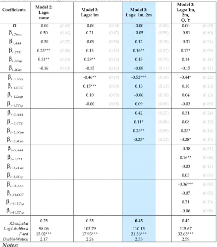
The results obtained for the distressed debt fund are shown in the following table 3. The results suggest that the most representative model for the fund’s strategy is model 3 with all but annual and quarterly lags included (for which the R2-adjusted value obtained is equal to 0.45) suggesting that these lags are not relevant for the fund’s strategy.

Table 3: E stimated Coefficients – Fund 2 (Distressed Debt)

Coefficients Model 2: Lags:

none

Model 3: Lags: 1m

Model 3: Lags: 1m, 2m

Model 3: Lags: 1m,

2m, Q, Y

α -0.00 (0.00) -0.00 (0.00) -0.00 (0.00) 0.00 (0.00)

Treas t,

β 0.50 (0.64) 0.21 (0.82) -0.05 (0.59) -0.81 (0.80)

AAA t,

β -0.30 (0.37) -0.09 (0.28) 0.12 (0.19) -0.31 (0.24)

CCC t,

β 0.23*** (0.06) 0.13 (0.12) 0.16** (0.07) 0.17* (0.09)

LCap t,

β 0.31** (0.14) 0.28** (0.12) 0.13 (0.15) 0.14 (0.14)

SCap t,

β -0.16 (0.10) -0.15 (0.12) -0.08 (0.11) -0.15 (0.11)

AAA t−1,

β -0.46** (0.19) -0.52*** (0.18) -0.44* (0.22)

CCC t−1,

β 0.15*** (0.05) 0.13 (0.13) 0.18 (0.13)

Lcap t−1,

β 0.10 (0.09) -0.06 (0.10) 0.04 (0.13)

SCap t−1,

β -0.00 (0.05) 0.09 (0.08) -0.03 (0.09)

AAA t−2,

β 0.42 (0.27) 0.31 (0.24)

CCC t−2,

β 0.11* (0.06) 0.08 (0.13)

LCap t−2,

β 0.25** (0.09) 0.23* (0.12)

SCap t−2,

β -0.23* (0.12) -0.28* (0.15)

AAA t−3,

β -0.38 (0.31)

CCC t−3,

β 0.16** (0.06)

LCap t−3,

β -0.03 (0.11)

SCap t−3,

β 0.03 (0.07)

AAA t−11,

β -0.36*** (0.09)

CCC t−11,

β -0.07 (0.05)

LCap t−11,

β 0.21 (0.13)

SCap t−11,

β -0.06 (0.08)

R2-adjusted 0.25 0.35 0.45 0.42

L og-L ik elihood 98.06 103.79 110.15 115.67

F-test 15.02*** 17.93*** 21.56*** 32.65***

Durbin-Watson 2.17 2.24 2.33 2.59

Notes:

§ Standard Deviations are in parentheses.

§ Significance levels: * significant at 10%; ** significant at 5%; *** significant at 1%

negative coefficients, respectively) whereas the radar graph provides a snapshot of the different magnitudes of these exposures.

Graph 3: Fund 2 (Distressed Debt) Asset Class E xposures and the Style Radar

Style of Fund 2 - Distressed Debt

-0.0033 -0.0450

0.1180 0.1560 0.1270 -0.0770

-0.5180

0.1320 -0.0630

0.0900

0.4200 0.1130

0.2480 -0.2250

-1 0 1

Alpha

US Treasury Bills 3m BoA ML AAA BoA ML CCC DJ Large Cap DJ Small Cap Lag1(BoA ML AAA) Lag1(BoA ML CCC) Lag1(DJ Large Cap) Lag1(DJ Small Cap) Lag2(BoA ML AAA) Lag2(BoA ML CCC) Lag2(DJ Large Cap) Lag2(DJ Small Cap)

-0.6 -0.5 -0.4 -0.3 -0.2 -0.1 0.0 0.1 0.2 0.3 0.4 0.5

Alpha

US Treasury Bills 3m

BoA ML AAA

BoA ML CCC

DJ Large Cap

DJ Small Cap

Lag1(BoA ML AAA)

Lag1(BoA ML CCC) Lag1(DJ Large Cap)

Lag1(DJ Small Cap) Lag2(BoA ML AAA) Lag2(BoA ML CCC)

Lag2(DJ Large Cap)

The results obtained for the hedge fund are shown in the table 4 below. Model three has the highest R2 score, being retained as the most relevant to explain the fund’s strategy. Two-months lag coefficients are predicted to be statistically and significantly different from zero.

Table 4: E stimated Coefficients – Fund 3 (H edge Fund)

Coefficients Model 2: Lags:

none

Model 3: Lags: 1m

Model 3: Lags: 1m, 2m

Model 3: Lags: 1m,

2m, Q, Y

α

Treas t,

β 0.33 (0.89) -0.21 (0.76) -0.78 (0.75) -0.04 (0.65)

AAA t,

β 0.17 (0.23) 0.05 (0.20) -0.18 (0.23) 0.02 (0.10)

CCC t,

β 0.37*** (0.08) 0.43*** (0.13) 0.56*** (0.12) 0.72*** (0.06)

LCap t,

β 0.55*** (0.12) 0.50*** (0.12) 0.48*** (0.13) 0.38*** (0.11)

SCap t,

β -0.29*** (0.07) -0.27*** (0.07) -0.32*** (0.08) -0.29*** (0.07)

AAA t−1,

β 0.13 (0.23) -0.25 (0.27) 0.08 (0.19)

CCC t−1,

β -0.03 (0.12) 0.08 (0.12) 0.01 (0.06)

Lcap t−1,

β 0.17 (0.14) 0.12 (0.10) 0.07 (0.07)

SCap t−1,

β -0.15 (0.13) -0.25*** (0.09) -0.23*** (0.05)

AAA t−2,

β -0.39 (0.25) -0.47*** (0.13)

CCC t−2,

β -0.14** (0.07) -0.32*** (0.06)

LCap t−2,

β 0.41** (0.15) 0.27*** (0.10)

SCap t−2,

β -0.28** (0.10) -0.10 (0.07)

AAA t−3,

β 0.97*** (0.15)

CCC t−3,

β -0.07 (0.05)

LCap t−3,

β 0.30*** (0.10)

SCap t−3,

β -0.06 (0.07)

AAA t−11,

β -0.33** (0.16)

CCC t−11,

β 0.01 (0.03)

LCap t−11,

β 0.09 (0.12)

SCap t−11,

β -0.02 (0.08)

R2-adjusted 0.60 0.59 0.66 0.79

L og-L ik elihood 106.05 107.57 114.61 132.45

F-test 35.62*** 26.59*** 36.41*** 196.81***

Durbin-Watson 1.58 1.75 2.01 2.03

Notes:

§ Standard Deviations are in parentheses.

§ Significance levels: *-significant at 10%; **-significant at 5%; ***-significant at 1%

Graph 4: Fund 3 (H edge Fund) Asset Class E xposures and the Style Radar

Style of Fund 3 - Hedge Fund

-0,01 -0,04

0,02

0,718 0,38

-0,29

0,08 0,01

0,07 -0,23

-0,47 -0,32

0,28 -0,10

0,97 -0,07

0,30 -0,06

-0,33

0,01 0,09 -0,02

-1,0 -0,5 0,0 0,5 1,0

Alpha

US Treasury Bills 3m BoA ML AAA BoA ML CCC DJ Large Cap DJ Small Cap Lag1(BoA ML AAA) Lag1(BoA ML CCC) Lag1(DJ Large Cap) Lag1(DJ Small Cap) Lag2(BoA ML AAA) Lag2(BoA ML CCC) Lag2(DJ Large Cap) Lag2(DJ Small Cap) LagQ(BoA ML AAA) LagQ(BoA ML CCC) LagQ(DJ Large Cap) LagQ(DJ Small Cap) LagY(BoA ML AAA) LagY(BoA ML CCC) LagY(DJ Large Cap) LagY(DJ Small Cap)

-0,6 -0,4 -0,2 0,0 0,2 0,4 0,6 0,8 1,0

Alpha

US Treasury Bills 3m

BoA ML AAA

BoA ML CCC

DJ Large Cap

DJ Small Cap

Lag1(BoA ML AAA)

Lag1(BoA ML CCC)

Lag1(DJ Large Cap)

Lag1(DJ Small Cap)

Lag2(BoA ML AAA) Lag2(BoA ML CCC)

Lag2(DJ Large Cap) Lag2(DJ Small Cap) LagQ(BoA ML AAA) LagQ(BoA ML CCC) LagQ(DJ Large Cap) LagQ(DJ Small Cap)

LagY(BoA ML AAA) LagY(BoA ML CCC)

In conclusion, comparing the results obtained from the analysis of different asset-class exposures models, we observe that model 3 provides, among the three models, the greatest level of decomposition of the portfolio performance onto asset class exposures, considering different levels of systematic risks and different time lagged effects. The richness of this model, which accounts for time lags, allows us to capture market-adjustment effects at a very low cost in terms of model specification. The easiness of use of this method makes it extremely attractive to the practitioner, from two viewpoints: implementation and interpretation of results. On one side, the multi-benchmark approach contributes to overcome the difficulties related to the subjective and, most of the times, unilateral choice of “the most appropriate benchmark” which has been criticized by many authors. On the other side, the use of a limited set of benchmarks keeps the model tractable and helps us avoiding the difficulties encountered by many PCA-like methods, containing potentially a very large set of (even very similar) indexes, when it comes to give an explanation to coefficients suggesting opposite strategies (e.g. long vs. short positions) on very similar benchmarks (such as AA Corporates and AAA Corporates Indexes, or Indexes of B and CCC-ranked securities). In terms of performance, this implies that traditional rankings of the funds based on the single-index based metrics could differ substantially.

6. Results Obtained from the Investment Style Models 4 and 5

In the following we discuss the results obtained from the estimation of the investment style models 4 (without lags) and 5 (with lags), in which index lagged returns are introduced gradually: first, the quarter effects and then, the annual effects.

Results for the mezzanine fund indicate that the best model replicating the strategy of this fund is the model 5 with all the three lags included. In fact R2-adjusted almost doubles in this model (from 0.16 to 0.31) when compared to the same metric obtained from the estimation of model 4, with no lags. The log-likelihood of the model also improves significantly. Following the results in the last column, the strategy of this fund can be summarized as follows:

§ Take short-like positions on the convertible arbitrage risk (β1,t) and the event driven risk

arbitrage (β3,t), with a following up of the latter on a quarterly and annual basis (β3,t−3

and β3,t−11);

§ Take long positions on the dedicated short-bias risk factor (β2,t), event driven distressed

securities (β4,t), fixed income arbitrage (β7,t) and global macroeconomic bets (β5,t) with

a following-up of the latter on a quarterly (β5,t−3) and annual basis (β5,t−11);

Table 5 – E stimated Coefficients for Fund 1 (Mezzanine) Coefficients Model 4: Lags: none Model 5: Lags: Q Model 5: Lags: Q, Y

α 0.00 (0.02) 0.01 (0.02) 0.01 (0.02)

t

, 1

β -4.51*** (1.22) -4.92*** (1.50) -5.73*** (1.48)

t

, 2

β 0.52 (0.55) 1.18** (0.51) 1.33** (0.49)

t

, 3

β -3.04 (2.46) -2.46 (2.11) -3.72** (1.66)

t

, 4

β 3.17 (1.78) 3.93** (1.75) 5.74** (2.24)

t

, 5

β 3.34 (2.24) 2.56 (1.68) 3.18** (1.24)

t

, 6

β 0.43 (1.35) 1.03 (1.09) 0.47 (0.83)

t

, 7

β 2.86*** (0.88) 2.74** (1.03) 3.21*** (0.84)

t

, 8

β -0.10 (0.21) 0.01 (0.19) 0.06 (0.20)

t

, 9

β -0.69 (0.64) -0.70 (0.54) -0.79 (0.50)

3 , 1t−

β -1.60 (1.15) -1.24 (1.14)

3 , 2t−

β -0.32 (0.47) -0.51 (0.52)

3 , 3t−

β -6.12*** (2.21) -5.74*** (1.86)

3 , 4t−

β 2.37 (1.66) 2.25 (1.57)

3 , 5t−

β 3.80** (1.42) 5.08*** (1.81)

3 , 6t−

β 0.02 (0.99) -1.03 (1.07)

3 , 7t−

β 0.22 (1.36) -0.22 (1.09)

3 , 8t−

β 0.27 (0.26) 0.02 (0.24)

3 , 9t−

β -1.50** (0.56) -1.88** (0.73)

11 , 1t−

β 0.23 (0.86)

11 , 2t−

β -0.65 (0.53)

11 , 3t−

β -5.41*** (1.47)

11 , 4t−

β 0.39 (1.04)

11 , 5t−

β 2.36* (1.78)

11 , 6t−

β -0.22 ()

11 , 7t−

β -0.45 (0.82)

11 , 8t−

β 0.19 (0.18)

11 , 9t−

β -1.25*** (0.38)

R2-adjusted 0.16 0.29 0.31

L og-L ik elihood 43.95 54.33 63.43

F-test 9.70*** 27.24*** 46.33***

Durbin-Watson 0.71 1.12 1.31

Notes:

§ Standard Deviations are in parentheses.

The following table shows the results obtained for the distressed debt fund. Interesting to remark that this method did not produce significant enough coefficients to explain the returns of our distressed debt fund within acceptable error limits (i.e. with probability of predicting unbiased coefficients of at least 90%) with just a few exceptions. This might be not be such a surprising result since we can reasonably argue that, in fact, the analyzed distressed debt fund would not usually adopt non-linear strategies such as convertible arbitrage, risk arbitrage, etcetera, as to be comparable to a hedge fund.

Table 6 – E stimated Coefficients for Fund 2 (Distressed Debt) Coefficients Model 4: Lags: none Model 5: Lags: Q Model 5: Lags: Q, Y

α

t

, 1

β 0.11 (0.21) 0.42 (0.35) 0.45 (0.11)

t

, 2

β 0.05 (0.09) 0.11 (0.07) 0.16 (0.14)

t

, 3

β -0.81 (0.63) 0.04 (0.58) 0.44 (0.58)

t

, 4

β 1.06* (0.62) 0.30 (0.40) 0.40 (0.24)

t

, 5

β -0.09 (0.34) -0.06 (0.31) 0.16 (0.64)

t

, 6

β 0.02 (0.24) -0.01 (0.27) 0.07 (0.83)

t

, 7

β 0.02 (0.19) -0.28 (0.23) -0.71** (0.01)

t

, 8

β -0.09 (0.07) 0.10* (0.05) 0.13*** (0.01)

t

, 9

β -0.10 (0.12) -0.01 (0.12) -0.23 (0.24)

3 , 1t−

β 0.47 (0.33) 0.35 (1.26)

3 , 2t−

β 0.07 (0.10) -0.01 (0.90)

3 , 3t−

β -0.39 (0.51) -0.11 (0.87)

3 , 4t−

β 0.32 (0.30) 0.07 (0.87)

3 , 5t−

β 0.43 (0.46) 0.06 (0.91)

3 , 6t−

β 0.12 (0.39) 0.11 (0.77)

3 , 7t−

β -0.39 (0.42) 0.07 (0.82)

3 , 8t−

β 0.01 (0.07) 0.09 (0.22)

3 , 9t−

β -0.11 (0.13) 0.04 (0.85)

11 , 1t−

β -0.25 (0.32)

11 , 2t−

β -0.01 (0.89)

11 , 3t−

β 0.77 (0.24)

11 , 4t−

β 0.40 (0.13)

11 , 5t−

β -0.17 (0.59)

11 , 6t−

β 0.37 (0.42)

11 , 7t−

β -0.61** (0.03)

11 , 8t−

β 0.04 (0.47)

11 , 9t−

β 0.05 (0.72)

R2-adjusted 0.22 0.27 0.14

L og-L ik elihood 99.59 107.56 113.64

F-test 44.44*** 143.47*** 75.60***

Durbin-Watson 2.25 2.74 2.66

Notes:

§ Standard Deviations are in parentheses.

The following table shows the results obtained for the hedge fund. The most representative model in this case is model 5 with quarterly lags (R2-adjusted value is 0.69) suggesting that the annual lags are not representative for the hedge fund’s strategy. Most coefficients are highly significant (with a probability of 99%).

Table 7 – E stimated Coefficients for Fund 3 (H edge Fund)

Coefficients Model 4: Lags: none Model 5: Lags: Q Model 5: Lags: Q, Y

α

t

, 1

β -0.52 (0.39) -1.02*** (0.35) -1.02*** (0.30)

t

, 2

β 0.14 (0.13) 0.28** (0.13) 0.21* (0.11)

t

, 3

β -0.25 (0.61) 0.17 (0.61) 0.71 (0.61)

t

, 4

β 0.92*** (0.27) 1.37*** (0.34) 1.61*** (0.35)

t

, 5

β 0.49 (0.40) 0.04 (0.30) 0.33 (0.25)

t

, 6

β -0.01 (0.41) 0.15 (0.41) -0.24 (0.27)

t

, 7

β 1.18*** (0.30) 1.57*** (0.22) 1.49*** (0.23)

t

, 8

β -0.05 (0.04) -0.13*** (0.03) -0.11** (0.04)

t

, 9

β -0.19 (0.12) -0.11 (0.11) -0.19 (0.16)

3 , 1t−

β 0.01 (0.24) 0.07 (0.26)

3 , 2t−

β 0.11* (0.06) 0.12* (0.07)

3 , 3t−

β -0.86** (0.37) 0.20 (0.65)

3 , 4t−

β 0.33 (0.28) 0.21 (0.33)

3 , 5t−

β 0.77** (0.30) 0.32 (0.44)

3 , 6t−

β -0.01 (0.24) -0.25 (0.26)

3 , 7t−

β -0.61** (0.25) -0.29 (0.34)

3 , 8t−

β 0.08 (0.05) -0.02 (0.08)

3 , 9t−

β -0.27* (0.15) -0.11 (0.14)

11 , 1t−

β 0.26 (0.21)

11 , 2t−

β -0.11 (0.10)

11 , 3t−

β -1.32*** (0.41)

11 , 4t−

β 0.29 (0.44)

11 , 5t−

β 0.47 (0.34)

11 , 6t−

β 0.20 (0.20)

11 , 7t−

β -0.36* (0.17)

11 , 8t−

β -0.02 (0.04)

11 , 9t−

β 0.04 (0.15)

R2-adjusted 0.66 0.69 0.66

L og-L ik elihood 112.16 120.73 127.87 F-test 48.30*** 161.13*** 946.25***

Notes:

§ Standard Deviations are in parentheses.

§ Significance levels: *-significant at 10%; **-significant at 5%; ***-significant at 1%

7. Conclusions

We believe that the assumption of stochastic returns is not always the best in class. By assuming a stochastic distribution of returns when an illiquid fund’s holdings are evaluated on a quarterly basis and interpolated on a monthly basis, or when the evaluation process is made ex-post (i.e. the current quarter/ month for the previous ones) the practitioner may fall into the risk of a “Type I error” in which a false positive error (with null hypothesis of stochastic returns) in finance causes “unnecessary worry” or explanation of the return series through a large set of risk factors.

The easiness of use of both methods we proposed in this paper makes them extremely attractive to the practitioner, from at least two viewpoints: implementation and interpretation of results. On one side, the multi-benchmark approach contributes to overcome the difficulties related to the subjective and, most of the times, unilateral choice of “the most appropriate benchmark” which has been criticized by many authors. On the other side, the use of a limited set of benchmarks keeps the model tractable and helps us avoiding the difficulties encountered by many PCA-like methods, containing potentially a very large set of redundant, correlated indexes, when it comes to give an explanation to coefficients suggesting opposite strategies (e.g. long vs. short positions) on very similar benchmarks (for example, if the method indicates a short position on AA Corporates and a long position on AAA Corporates, or Indexes of B and CCC-ranked securities). Moreover, the use of simple tests such as the R2-adjusted of the equation, variation-inflated-test (VIF) and likelihood ratio tests (LR) as main criteria for the identification of the best-in-class models are easily implementable.

A combined analysis using the versions of models 3 and 5 with the optimal number of lags (e.g. the model corresponding to the highest correlation and coefficients statistically significant at a 95% confidence level at least) when evaluating the portfolios in this complex class of investments, would allow us to capture:

§ the fund’s exposures to different asset classes, thus, to different types of risk factors such as duration, interest rate, size effects, etc.

§ non-linear effects in the fund strategy such as market-timing related effects, pure style patterns comparable to the ones undertaken by hedge fund managers.

8. Appendix

Table 1: Summary Statistics

(Monthly Observations: June 2008 – September 2012)

Denomination Avg.

Return Std. Dev.

Downside Std. Dev.

Sharpe Ratio

Sortino Ratio

F UNDS:

Mezzanine Fund 0.002 0.453 0.319 0.004 0.006

Distressed Debt Fund 0.238 0.280 0.162 0.851 1.472

Hedge Fund -0.146 0.149 0.131 -0.978 -1.112

INDE XE S:

US 1 year Treasury Bills 0.028 0.014 0.000 1.931 -

9. Bibliography

1. Bera, A.K., and Jarque C.M. (1981): “An efficient large sample test for normality of

observations and regression residuals” Australian National University, working papers in

econometrics, 40, Canberra.

2. E lton, Gruber, Das and Hlavka’ (1993): “E fficiency with costly information: a

reinterpretation of evidence from managed portfolios”, The review if Financial Studies,

vol.6, n.1, p. 1-22.

3. Fung W. and Hsieh D.A. (2000): “Performance characteristics of hedge funds and

commodity funds: natural versus spurious biases”, Journal of Financial and Quantitative

Analysis, vol. 35, issue 3, p- 291-307.

4. Greene, W. (2007) : E conometric Analysis : 6th E d., Pearson E ducation pp.1211.

5. Grinblatt M., Titman S., and Wermers R. (1995): “Momentum investment strategies,

portfolio performance and herding: a study of mutual fund behavior”, The American

E conomic Review, vo. 85, issue 5 pp.1088-1105.

6. Henriksson, R., and Merton, R. (1981): “On market timing and Investment

performance”, The Journal of Business, vol. 54 n.4 pp.513-533.

7. Ljung, G.M. and Box G.E .P. (1978): “On a measure of lack of fit in time series analysis

models”, Biometrika, vol. 65 N.2 p. 297-303.”

8. Lhabitant, F. S. (2001): “Assessing market risk for hedge funds and hedge fund

portfolios,” Journal of Risk Finance, 2001, p.1-17.

9. Lhabitant, F. S. (2003): “Assessing hedge fund investments: the role of pure style

indices”, E DHEC Risk and Asset Management Research Center WP series.

10.Liang B. (2003): “On the performance of alternative investments”, CTAs, Hedge Funds,

and FohF, working paper.

11.Le Sourd, V. (2007): “Performance measurement for traditional investment”, E dhec

Working Paper Series.

12.Sharpe, W.F. (1992): “Asset allocation: management style and performance measurement.

An asset class factor model can help make order out of the chaos” reprinted from the

Journal of Portfolio Management 1992, p. 7-19.

13.Index Databases: BoA Merrill Lynch Index Database; Standard and Poor’s Index