Exploring Deep Belief Network for Chinese Relation Extraction

Exploring Deep Belief Network for Chinese Relation Extraction

Yu Chen

, Wenjie Li

, Yan Liu

, Dequan Zheng

, Tiejun Zhao

School of Computer Science and Technology, Harbin Institute of Technology, China

{chenyu, dqzheng, tjzhao}@mtlab.hit.edu.cn

2

Department of Computing, The Hong Kong Polytechnic University, Hong Kong

{cswjli, csyliu}@comp.polyu.edu.hk

Abstract

Relation extraction is a fundamental task in information extraction that identifies the semantic relationships between two entities in the text. In this paper, a novel model based on Deep Belief Network (DBN) is first presented to detect and classify the relations among Chinese entities. The experiments conducted on the Automatic Content Extraction (ACE) 2004 dataset demonstrate that the proposed approach is effective in handling high dimensional feature space including character N-grams, entity types and the position information. It outperforms the state-of-the-art learning models such as SVM or BP neutral network.

1

Introduction

Information Extraction (IE) is to automatically pull out the structured information required by the users from a large volume of plain text. It normally includes three sequential tasks, i.e., entity extraction, relation extraction and event extraction. In this paper, we limit our focus on relation extraction.

In early time, pattern-based approaches were the main focus of most research studies in relation extraction. Although pattern-based approaches achieved reasonably good results, they have some obvious flaws. It requires expensive handcraft work to assemble patterns and not all relations can be identified by a set of reliable patterns (Willy Yap, 2009). Also, once the interest of task is transferred to a different domain or a different language, patterns have to be revised or even rewritten. That is to say, the discovered patterns are

heavily dependent on the task in a specific domain or on a particular corpus.

Naturally, a vast amount of work was spent on feature-based machine learning approaches in later years. In this camp, relation extraction is typically cast as a classification problem, where the most important issue is to train a model to scale and measure the similarity of features reflecting relation instances. The entity semantic information expressing relation was often formulated as the lexical and syntactic features, which are identical to a certain linear vector in high dimensions. Many learning models are capable of self-training and classifying these vectors according to similarity, such as Support Vector Machine (SVM) and Neural Network (NN).

Recently, kernel-based approaches have been developing rapidly. These approaches involved kernels of structure representations, like parse tree or dependency tree, in similarity calculation. In fact, feature-based approaches can be viewed as the special and simplified kinds of kernel-based approaches. They used dot-product as the kernel function and did not range over the intricate structure information (Ji, et al. 2009).

Relation extraction in Chinese received quite limited attention as compared to English and other western languages. The main reason is the unique characteristic of Chinese, such as more flexible grammar, lack of boundary information and morphological variations etc (Sun and Dong, 2009). Especially, the existing Chinese syntactic analysis tools at current stage are not yet reliable to capture the valuable structured information. It is urgent to develop approaches that are in particular suitable for Chinese relation extraction.

extraction. It is a neural network model developed under the deep learning architecture that is claimed by Hinton (2006) to be able to automatically learn a deep hierarchy of features with increasing levels of abstraction for the complex problems like natural language processing (NLP). It avoids assembling patterns that express the semantic relation information and meanwhile it succeeds to produce accurate model that is not confined to the parsing results.

The rest of this paper is structured in the following manner. Section 2 reviews the previous work on relation extraction. Section 3 presents task definition, briefly introduces the DBN model and the feature construction. Section 4 provides the experimental results. Finally, Section 5 concludes the paper.

2

Related Work

Over the past decades, relation extraction had come to a significant progress from simple pattern-based approaches to adapted self-training machine learning approaches.

Brin (1998) used Dual Iterative Pattern Relation Expansion, a bootstrapping-based system, to find the largest common substrings as patterns. It had the ability of searching patterns automatically and was good for large quantity of uniform contexts. Chen (2006) proposed graph algorithm called label propagation, which transferred the pattern similarity to probability of propagating the label information from any vertex to its nearby vertices. The label matrix indicated the relation type.

Feature-based approaches utilized the linear vector of carefully chosen lexical and syntactic features derived from different levels of text analysis and ranging from part-of-speech (POS) tagging to full parsing and dependency parsing (Zhang 2009). Jing and Zhai (2007) defined a unified graphic representation of features that served as a general framework in order to systematically explore the information at diverse levels in three subspaces and finally estimated the effectiveness of these features. They reported that the basic unit feature was generally sufficient to achieve state-of-art performance. Meanwhile, over-inclusion complex features were harmful.

Kernel-based approaches utilize kernel functions on structures between two entities, such as sequences and trees, to measure the similarity between two relation instances. Zelenok (2003) applied parsing tree kernel function to distinguish whether there was an existing relationship between two entities. However, they limited their task on Person-affiliation and organization-location.

The previous work mainly concentrated on relation extraction in English. Relatively, less attention was drawn on Chinese relation extraction. However, its importance is being gradually recognized. For instance, Zhang et al. (2008) combined position information, entity type and context features in a feature-based approach and Che (2005) introduced the edit distance kernel over the original Chinese string representation.

DBN is a new feature-based approach for NLP tasks. According to the work by Hinton (2006), DBN consisted of several layers including multiple Restricted Boltzmann Machine (RBM) layers and a Back Propagation (BP) layer. It was reported to perform very well in many classification problems (Ackley, 1985), which is from the origin of its ability to scale gracefully and be computationally tractable when applied to high dimensional feature vectors. Furthermore, to against the combinations of feature were intricate, it detected invariant representations from local translations of the input by deep architecture.

3

Deep Belief Network for Chinese

Relation Extraction

3.1 Task Definition

Relation extraction, promoted by the Automatic Content Extraction (ACE) program, is a task of finding predefined semantic relations between pairs of entities from the texts. According to the ACE program, an entity is an object or a set of objects in the world while a relation is an explicitly or implicitly stated relationship between entities. The task can be formalized as:

1 2

( , , )

e e s



r

between them. We call the triple

( , , )

e e s

Role: it represents an affiliation between a Person entity and an Organization, Facility, or GPE (a Geo-political entity) entities. Part: it represents the part-whole relationship

between Organization, Facility and GPE entities.

At: it represents that a Person, Organization, GPE, or Facility entity is location at a Location entities.

Near: it represents the fact that a Person, Organization, GPE or Facility entity is near (but not necessarily “At”) a Location or GPE entities.

Social: it represents personal and professional affiliations between Person entities.

3.2 Deep Belief Networks (DBN)

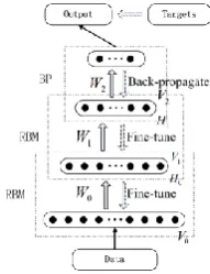
DBN often consists of several layers, including multiple RBM layers and a BP layer. As illustrated in Figure 1, each RBM layer learns its parameters independently and unsupervisedly. RBM makes the parameters optimal for the relevant RBM layer and detect complicated features, but not optimal for the whole model. There is a supervised BP layer on top of the model which fine-tunes the whole model in the learning process and generates the output in the inference process. RBM keeps information as more as possible when it transfers vectors to next layer. It makes networks to avoid local optimum. RBM is also adopted to ensure the efficiency of the DBN model.

Fig. 1. The structure of a DBN.

available at http://www.nist.gov/speech/tests/ace/.

Deep architecture of DBN represents many functions compactly. It is expressible by integrating different levels of simple functions (Y. Bengio and Y. LeCun). Upper layers are supposed to represent more “abstract” concepts that explain the input data whereas lower layers extract “low-level features” from the data. In addition, none of the RBM guarantees that all the information conveyed to the output is accurate or important enough. The learned information produced by preceding RBM layer will be continuously refined through the next RBM layer to weaken the wrong or insignificant information in the input. Multiple layers filter valuable features. The units in the final layer share more information from the data. This increases the representation power of the whole model. The final feature vectors used for classification consist of sophisticated features which reflect the structured information, promote better classification performance than direct original feature vector.

3.3 Restricted Boltzmann Machine (RBM)

In this section, we will introduce RBM, which is the core component of DBN. RBM is Boltzmann Machine with no connection within the same layer. An RBM is constructed with one visible layer and one hidden layer. Each visible unit in the visible layer V is an observed variable v_i while each hidden unit in

the hidden layer H is a hidden variable h_j. Its

joint distribution is

( , ) exp( ( , )) h Wv b x c hT T T p v h  E v h e   (2)

In RBM, 2

( , ) {0,1}v h  and  ( , , )W b c are the parameters that need to be estimated，W is the weight tying visible layer and hidden layer. b is the bias of units v and c is the bias of units h.

To learn RBM, the optimum parameters are obtained by maximizing the joint distribution

( , )

0 ( 1) ( ) log ( )

W

P v

W W

W 

 _  _

 (3)

where  is a parameter controlling the leaning rate. It determines the speed of W converging to the target.

Traditionally, the Monte Carlo Markov chain (MCMC) is used to calculate this kind of gradient.

0 0

log ( , )p v h

h v h v

w

 

 _{ }

 (4)

where log ( , )p v h is the log probability of the data. 0 0

h v denotes the multiplication of the average over the data states and its relevant sample in hidden unit. _{h v}  _{denotes the}

multiplication of the average over the model states in visible units and its relevant sample in hidden units.

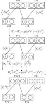
Fig. 2. Learning RBM with CD-based gradient estimation

However, MCMC requires estimating an exponential number of terms. Therefore, it typically takes a long time to converge to

h v  . Hinton (2002) introduced an alternative

algorithm, i.e., the contrastive divergence (CD) algorithm, as a substitution. It is reported that CD can train the model much more efficiently than MCMC. To estimate the distribution p x( ), CD considers a series of distributions {p x_n( )}

which indicate the distributions in n steps. It approximates the gap of two different Kullback-Leiler divergences as

0

( || ) ( || )

n n

CD KL p p KL p p (5)

Maximizing the log probability of the data is exactly the same as minimizing the Kullback– Leibler divergence between the distribution of the data p₀ and the equilibrium distribution

p defined by the model.

In our experiments, we set n to be 1. It means that in each step of gradient calculation, the estimate of the gradient is used to adjust the weight of RBM as Equation 6.

0 0 1 1 log ( , )p v h

h v h v W

 _{ }

 (6)

Figure 2 below illustrates the process of learning RBM with CD-based gradient estimation.

3.4 Back-Propagation (BP)

The RBM layers provide an unsupervised analysis on the structures of data set. They automatically detect sophisticated feature vectors. The last layer in DBN is the BP layer. It takes the output from the last RBM layer and applies it in the final supervised learning process. In DBN, not only is the supervised BP layer used to generate the final categories, but it is also used to fine-tune the whole network. Specifically speaking, when the BP layer is changed during its iterating process, the changes are passed to the other RBM layers in a top-to-bottom sequence.

3.5 The Feature Set

DBN is able to detect high level hidden features from lexical, syntactic and/or position characteristic. As mentioned in related work, over-inclusion complex features are harmful. We therefore involve only three kinds of low level features in this study. They are described below.

3.5.1 Character-based Features

Since Chinese text is written without word boundaries, the word-level features are limited by the efficiency of word segmentation results. In the paper presented by H. Jing (2003) and some others, they observed that pure character-based models can even outperform word-character-based models. Li et al.’s (2008) work relying on character-based features also achieved significant performance in relation extraction. We denote the character dictionary as D={d1,

an e, it’s character-based feature vector is V(e)={ v1, v2, …, vN }. Each unit vi can be

valued as Equation 8.

   

  

0 1

e d

e d v

i i

i (7)

3.5.2 Entity Type Features

According to the ACE 2004 guideline, there are five entity types in total, including Person, Organization, GPE, Location, and Facility. We recognize and classify the relation between the recognized entities. The entities in ACE 2004 corpus were labeled with these five types. Type features are distinctive for classification. For example, the entities of Location cannot appear in the Role relation.

3.5.3 Relative Position Features

We define three types of position features which depict the relative structures between the two entities, including Nested, Adjacent and Separated. For each relation candidate triple ( , , )e e s_{1 2} , let .starte and e.end denote the starting and end positions of

e

Type Condition

Nested ( .start, .end)ei ei ( .start, ej ej.end) Adjacent ei.end= .start-1ej

Separated ( .start< .start)&( .end+1< .start)ei ej ei ej

Table 1. The internal postion structure features between two named entities

We combine the character-based features of two entities, their type information and position information as the feature vector of relation candidate.

3.6 Order of Entity Pair

A relation is basically an order pair. For example, “Bank of China in Hong Kong” conveys the ACE-style relation “At” between two entities “Bank of China (Organization)” and “Hong Kong (Location)”. We can say that Bank of China can be found in Hong Kong, but not vice verse. The identified relation is said to be correct only when both its type and the order of the entity pair are correct. We don’t explicitly incorporate such order

restriction as an individual feature but use the specified rules to sort the two entities in a relation once the relation type is recognized. As for those symmetric relation types, the order needs not to be concerned. Either order is considered correct in the ACE standard. As for those asymmetric relation types, we simply select the first (in adjacent and separated structure) or outer (in nested structures) as the first entity. In most cases, this treatment leads to the correct order. We also make use of entity types to verify (and rectify if necessary) this default order. For example, considering “At” is a relation between a Person, Organization, GPE, or Facility entity and a Location entity, the Location entity must be placed after the Person, Organization, GPE, or Facility entity in a relation.

4

Experiments and Evaluations

4.1 Experiment Setup

The experiments are conducted on the ACE 2004 Chinese relation extraction dataset, which consists of 221 documents selected from broadcast news and newswire reports. There are 2620 relation instances and 11800 pairs of entities have no relationship in the dataset. The size of the feature space is 3017.

We examine the proposed DBN model using 4-fold cross-validation. The performance is measured by precision, recall, and F-measure.

2*Precision*Recall -measure=

Precision+Recall

F (8)

In the following experiments, we plan to test the effectiveness of the DBN model in three ways:

Detection Only: For each relation candidate, we only recognize whether there is a certain relationship between the two entities, no matter what type of relation they hold. Detection and Classification in Sequence:

For each relation candidate, when it is detected to be an instance of relation, it proceeds to detect the type of the relation the two entities hold.

the two entities. In this way, the processes of detection and classification are combined.

We will compare DBN with a well-known Support Vector Machine model (labeled as SVM in the tables) and a traditional BP neutral network model (labeled as NN (BP only)). Among them, SVM has been successfully applied in many classification applications. We use the LibSVM toolkit2 to implement the SVM model.

4.2 Evaluation on Detection Only

We first evaluate relation detection, where only two output classes are concerned, i.e. NULL (which means no relation recognized) and RELATION. The parameters used in DBN, SVM and NN (BP only) are tuned experimentally and the results with the best parameter settings are presented in Table 2. In each of our experiments, we test many parameters of SVM and chose the best set of that to show below.

Regarding the structure of DBN, we experiment with different combinations of unit numbers in the RBM layers. Finally we choose DBN with three RBM layers and one BP layer. And the numbers of units in each RBM layer are 2400, 1800 and 1200 respectively, which is the best size of each layer in our experiment. Our empirical results showed that the numbers of units in adjoining layers should not decrease the dimension of feature vector too much when casting the vector transformation. NN has the same structure as DBN. As for SVM, we choose the linear kernel with the penalty parameter C=0.3, which is the best penalty coefficient, and set the other parameters as default after comparing different kernels and parameter values.

Model Precision Recall F-measure DBN 67.8% 70.58% 69.16% SVM 73.06% 52.42% 61.04% NN (BP

only) 51.51% 61.77% 56.18%

Table 2. Performances of DBN, SVM and NN models for detection only

As showed in Table 2, with their best parameter settings, DBN performs much better

http://www.csie.ntu.edu.tw/~cjlin/libsvm/

than both SVM and NN (BP only) in terms of F-measure. It tells that DBN is quite good in this binary classification task. Since RBM is a fast approach to approximate global optimum of networks, its advantage over NN (BP only) is clearly demonstrated in their results.

4.3 Evaluation on Detection and Classification in Sequence

In the next experiment, we go one step further. If a relation is detected, we classified it into one of the 5 pre-defined relation types. For relation type classification, DBN and NN (BP only) have the same structures as they are in the first experiment. We adopt SVM linear kernel again and set C to 0.09 and other parameters as default. The overall performance of detection and classification of three models are illustrated in Table 3 below. DBN again is more effective than SVM and NN.

Model Precision Recall F-measure DBN 63.67% 59% 61.25% SVM 67.78% 47.43% 55.81% NN 61% 45.62% 52.2%

Table 3. Performances of DBN and other classification models for detection and classification in sequence

4.4 Evaluation on Detection and Classification in Combination

In the third experiment, we unify relation detection and relation type classification into one classification task. All the candidates are directly classified into one of the 6 classes, including 5 relation types and a NULL class. Parameter settings of the three models in this experiment are identical to those in the second experiment, except that C in SVM is set to 0.1.

Model Precision Recall F-measure DBN 65.8% 59.15% 62.3% SVM 75.25% 44.07% 55.59% NN (BP

only) 63.2% 45.7% 53.05%

Table 4. Performances of DBN, SVM and NN models for detection and classification in combination

advantages of DBN over the other two models are apparent. RBM approximates expected parameters rapidly and the deep DBN architecture yields stronger representativeness of complicated, efficient features.

Comparing the results of the second and the third experiments, SVM perform better (although not quite significantly) when detection and classification are in sequence than in combination. This finding is consistent with our previous work (to be added later). It can possibly be that preceding detection helps to deal with the severe unbalance problem, i.e. there are much more relation candidates that don’t hold pre-defined relations. However, DBN obtaining the opposite result cause by that the amount of examples we have is not sufficient for DBN to self-train itself well for type classification. We will further exam this issue in our feature work.

4.5 Evaluation on DBN Structure

Next, we compare the performance of DBN with different structures by changing the number of RBM layers. All the candidates are directly classified into 6 types in this experiment.

DBN Precision Recall F-measure 3 RBMs +

BP 65.8% 59.15% 62.3% 2 RBMs +

BP 65.22% 57.1% 60.09% 1 RBM +

BP 64.35% 55.5% 59.6%

Table 5. Performance RBM with different layers

The results provided in Table 5 show that the performance can be improved when more RBM layers are incorporated. Multiple RBM layers enhance representation power. Since it was reported by Hinton (2006) that three RBM layer is enough to detect the complex features and more RBM layer are of less help, we do not try to go beyond the three layers in this experiment. Note that the improvement is more obvious from two layers to three layers than from one layer to two layers.

4.6 Error Analysis

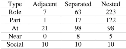
Finally, we provide the test results for individual relation types in Table 6. We can see that the proposed model performs better on “Role” and “Part” relations. When taking a closer look at their relation instance distributions, the instances of these two types comprise over 63% percents of all the relation instances in the dataset. Clearly their better results benefit from the amount of training data. It further implies that if we have more training data, we should be able to train a more powerful DBN. The samecharacteristic is also observed in Table 7 which shows the distributions of the identified relations against the gold standard. However, the sizes of “At” relation instances and “Role’ relation instances are similar, its result is much worse. We believe it is from the origin of that the position feature is not distinctive for “At” relation, as shown in Table 8. “Near” and “Social” are two symmetric relation types. Ideally, they should have better results. But due to quite small number of training examples, you can see that they are actually the types with the worst F-measure.

Type Precision Recall F-measure Role 65.19% 69.2% 67.14%

Part 67.86% 71.43% 69.59% At 51.15% 60% 55.22% Near 15.38% 33.33% 20.05% Social 25% 35.71% 29.41%

Table 6. Performance of DBN for each relation type

R P A N S Null Role (R) 191 1 5 0 0 96

Part (P) 1 95 12 0 0 32 At (A) 4 8 111 2 1 91 Near (N) 0 1 0 2 0 10 Social (S) 1 0 0 0 5 14

Table 7. Distribution of the identified relations

Type Adjacent Separated Nested

Role 7 63 223

Part 1 17 122

At 21 98 98

Near 0 8 5

Social 10 10 10

Table 8. Statistic of position feature

The main mistakes observed in Table 7 are wrongly classifying a “Part” relation as a “At” relations. We further inspect these 12 mistakes and find that it is indeed difficult to distinct the two types for the given entity pairs. Here is a typical example: entity 1: 美国民主党 (the Democratic Party of the United States, defined as an organization entity), entity 2: 美国 (the United States, defined as a GPE entity). Therefore, the major problem we have to face is how to effectively recall more relations. Given the limited training resources, it is needed to well explore the appropriate external knowledge or the Web resources.

5

Conclusions

In this paper we present our recent work on applying a novel machine learning model, namely Deep Belief Network, to Chinese relation extraction. DBN is demonstrated to be effective for Chinese relation extraction because of its strong representativeness. We conduct a series of experiments to prove the benefits of DBN. Experimental results clearly show the strength of DBN which obtains better performance than other existing models such as SVM and the traditional BP neutral network. In the future, we will explore if it is possible to incorporate the appropriate external knowledge in order to recall more relation instances, given the limited training resource.

References

Ackley D., Hinton G. and Sejnowski T. 1985. A learning algorithm for Boltzmann machines, Cognitive Science, 9.

Brin Sergey. 1998. Extracting patterns and relations from world wide web, In Proceedings of WebDB Workshop at 6th International Conference on Extending Database Technology (WebDB’98), 172-183.

Che W.X. Improved-Edit-Distance Kernel for Chinese Relation Extraction, In Dale, R.,Wong, K.-F., Su, J., Kwong, O.Y. (eds.) IJCNLP 2005.LNCS(LNAI). vol. 2651.

H. Jing, R. Florian, X. Luo, T. Zhang, A. Ittycheriah. 2003. How to get a Chinese name (entity): Segmentation and combination issues. In proceedings of EMNLP. 200-207.

Hinton, G.. 1999. Products of experts. In Proceedings of the Ninth International. Conference on Artificial Neural Networks (ICANN). Vol. 1, 1–6.

Hinton, G. E. 2002. Training products of experts by minimizing contrastive divergence, Neural Computation, 14(8), 1711–1800.

Hinton G. E., Osindero S. and Teh Y. 2006. A fast learning algorithm for deep belief nets, Neural Computation, 18. 1527–1554.

Ji Zhang, You Ouyang, Wenjie Li and Yuexian Hou. 2009. A Novel Composite Kernel Approach to Chinese Entity Relation Extraction. in Proceedings of the 22nd International Conference on the Computer Processing of Oriental Languages, Hong Kong, pp240-251.

Ji Zhang, You Ouyang, Wenjie Li, and Yuexian Hou. 2009. Proceedings of the 22nd International Conference on Computer Processing of Oriental Languages. 236-247. Jiang J. and Zhai C. 2007. A Systematic

Exploration of the Feature Space for Relation Extraction, In Proceedings of NAACL/HLT, 113–120.

Jinxiu Chen, Donghong Ji, Chew L., Tan and Zhengyu Niu. 2006. Relation extraction using label propagation based semi-supervised learning, InProceedings of ACL’06, 129–136. Li W.J., Zhang P., Wei F.R., Hou Y.X. and Lu, Q.

2008. A Novel Feature-based Approach to Chinese Entity Relation Extraction, In Proceeding of ACL 2008 (Companion Volume), 89–92

Sun Xia and Dong Lehong, 2009. Feature-based Approach to Chinese Term Relation Extraction. International Conference on Signal Processing Systems.

Willy Yap and Timothy Baldwin. 2009. Experiments on Pattern-based Relation Learning. Proceeding of the 18th ACM conference on Information and knowledge management. 1657-1660.

Y. Bengio and Y. LeCun. 2007. Scaling learning algorithms towards ai. Large-Scale Kernel Machines. MIT Press.

Zelenko D. Aone C and Richardella A. 2003. Kernel Methods for Relation Extraction, Journal of Machine Learning Research 2003(2), 1083–1106.