Fast Feedforward Non-parametric Deep Learning
Network with Automatic Feature Extraction
Plamen Angelov
, Fellow, IEEE
and Xiaowei Gu,
Student member, IEEE
School of Computing and Communications, Lancaster University
Lancaster, LA1 4WA, UK {p.angelov,x.gu3}@lancaster.ac.uk
Jose Principe,
Fellow, IEEE
Computational Neuro Engineering Laboratory, Department of Electrical and Computer Engineering,
University of Florida, Grainsville, FL, USA, [email protected]
Abstract— In this paper, a new type of feedforward non-parametric deep learning network with automatic feature extraction is proposed. The proposed network is based on human-understandable local aggregations extracted directly from the images. There is no need for any feature selection and parameter tuning. The proposed network involves nonlinear transformation, segmentation operations to select the most distinctive features from the training images and builds RBF neurons based on them to perform classification with no weights to train. The design of the proposed network is very efficient (computation and time wise) and produces highly accurate classification results. Moreover, the training process is parallelizable, and the time consumption can be further reduced with more processors involved. Numerical examples demonstrate the high performance and very short training process of the proposed network for different applications.
Keywords— deep learning; fast training; feedforward; feature extraction; learning network.
I. INTRODUCTION
Nowadays, with the very fast development of the electronic devices and information technologies, the number of images and videos uploaded to the websites and social media is increasingly growing. Other domains like industry [1], healthcare [2] as well as security [3] also have a very strong need of handling huge amounts of images and videos. As a result, image processing is now an increasingly popular research area [1]–[4].
Deep learning [5] is a hot research area attracting the attention of machine learning researchers as well as the public. Relying on extracting high level abstractions in data by using a multiple layer structure composed of linear and non-linear transformations, the published methods have presented very promising results in image processing [6]– [10]. Nonetheless, there are four major deficiencies in the current deep learning methods:
i) The features extracted and the steps to get them by the encoder-decoder methods have low level of human interpretability (are opaque) [5]–[8];
ii) The training process is off-line and requires a large
amount of time as well as complex computational resources [8]–[10];
iii) There are too many ad hoc decisions and parameters (the number of layers, neurons, parameter values) [6]–[10];
iv) The training process is not parallelisable [6]–[10]. These deficiencies largely hinder the acceptability of the deep learning network. Realising the fact that the success of deep neural networks (DNNs) is built upon huge amounts of numerical experiments with significant expertise, an alternative approach was proposed in [11] using the wavelet scattering convolution network as the descriptor to extract SIFT-type features from images and based on this to train the SVM or PCA classifiers. Although, this approach successfully avoids the ambiguous ad hoc decisions made in the DNNs design [6]–[10], the wavelet scattering convolution network actually requires the wavelets to be well defined in advance [11].
In this paper, we introduce a novel fast feedforward non-parametric deep learning method with automatic feature extraction. The proposed network is based on the local aggregations extracted directly from the images and has no parameters to train. As a result, the design process is very fast. The proposed network converts the extracted local aggregation matrices into vectors and involves a nonlinear mapping function to improve the distinctiveness of the identified local aggregations. Using the grid segmentation operation, the extracted local aggregations are divided into smaller blocks according to their original positions within the images. Since the blocks are independent from each other, multi-level parallelization is also possible. By selecting the most distinctive local aggregations within each block, the network is able to build a number of radical-basis function (RBF) neurons based on them and perform classification. Compared with the DNNs [6]–[10] and the alternative approach [11], the proposed network has the following advantages:
i) The extracted features are human understandable and can easily be visualised;
ii) The learning process is simple and fast, there are no iterations for parameter training;
Fig.1. Architecture of the fast feedforward deep learning network iii) The learning process is fully parallelisable.
The numerical examples clearly demonstrate that the proposed network is able to perform highly accurate classification after a very short learning process and it can be applied to various fields.
The remainder of this paper is organised as follows. The architecture of the proposed network for feature extraction is described in section II. The architecture of the network for predicting the class label is described in section III. The details of the training of the proposed network are presented in section IV. Numerical examples and discussion are given in section V. Section VI concludes the paper.
II. ARCHITECTURE OF THE PROPOSED NETWORK FOR
FEATURE EXTRACTION
The architecture of the proposed fast feedforward deep learning network up to the final, class prediction stage is depicted in Fig. 1. As it is shown in Fig.1, the proposed network has 6 layers plus the prediction layer. The first layer is for non-overlapping mean pooling with size 2 2 . The second layer is for extracting local aggregations as features from the pooled images. The third layer is nonlinear mapping layer. The forth layer is the segmentation layer. The fifth layer is for filtering out the overlapping/similar features extracted from images of different classes. The sixth layer includes the RBF neurons build based on the extracted local aggregations.
In the rest of this section, we will describe the novel characteristics of our method. In this paper, for simplicity, we only consider grayscale images with pixel values scaled into
0,1 . The size of the original images is denoted as2 2d d , and, thus, after the mean pooling, the size of images becomes d d .A. Local aggregations extraction layer
In this layer, the local aggregations within images are extracted. These are based on the gradients between the grey level values of the surrounding/neighboring pixels to a given pixel. In our method, the local aggregations for the pixel pi j, (i j, are the coordinates indicating the position of
this pixel within the image) is achieved by using a n n (n
is a small odd number) sliding window with a stride of 1
pixel, and the pixel pi j, is in the center of the sliding
window. The local aggregation around pi j, is expressed as: ,
,
c l i j
, , , , , ,
, 1, 1 , , 1, 1
1,
2 2 2 2 2
, , , , , ,
, , 1 , , , , 1
2 2
, ,
, , , ,
1,
, 1, 1 2 , 1
2 2
c l c l c l c l c l c l
i j i n j n i j n i j i n j n
i j
c l c l c l c l c l c l
i j i j n i j i j i j i j n
c l c l
c l c l i j n c l
i j
i j i n j n i j i n
p p p p p p
p p p p p p
p p
p p p p
,
1 , 2 2
c l n j
, , , , , 1 , 1 , , 1 1 , 2 , , , , , , , 2
c l c l c l c l c l
n i j i j i j n
i j i j
a a a a a (1)
where , ,
c l i j k a
T
, , , , , ,
, 1, , 3, , 1,
2 2 2
, , ,
c l c l c l c l c l c l
i j i n j k i j i n j k i j i n j k
p p p p p p
;
c (c1,2,...,C) is the class label of the image; C is the number of classes in the image dataset; l is the index of the image within its class.
By using the gradients of the grey level as local aggregations, the local features, i.e. edges, shapes, are preserved, while the influence of illumination is reduced. In order to get the most effective local aggregations, we only consider valid features ,
,
c l i j
which have more than half of its elements being non-zero. The ,
,
c l i j
that fail to meet this requirement are being discarded.
After the n n local aggregations are extracted, the matrix is converted into a long vector by concatenating different rows from the local aggregation matrix. Because, the center of each aggregation is always equal to zero, we can omit the center in the vector, and, thus, obtain a
n2 1 1local aggregation vector:
TT T
T T
, , , , ,
, , 1 , , 1 , 1
2 2
, , , , ,
c l c l c l c l c l
i j i jn i j i j i jn
a a a a
(a)
x (b) d x dx
Fig.2. The curves of the nonlinear mapping function and its gradient
Fig.3. The architecture of the proposed network for evaluation
where , , , , ,
, , 1, , 1, 2 , , ,
c l c l c l c l c l
i j pi jpin j k pi jpi j k
a
T , , , , , 1, , 1,
2
, ,
c l c l c l c l
i j i j k i j i n j k
p p p p
.
Due to the fact that the gradients of grey level values are not available in all directions in the edges of the images, we discard the pixels that do not have full/whole local aggregations around the edges. Thus, after the local aggregation extraction, the size of images becomes
2
(d n 1) (d n 1) n 1 .
B. Nonlinear Projection Layer
After the extraction of the local aggregations, their values are limited to the range
1,1 because the pixel grey level values are normalized into the range
0,1 . This makes it hard to linearly separate the classes. In this paper, we employ the following nonlinear one-to-one mapping function to amplify the differences between various local aggregations:
x sgn( ) exp 1 sgn( )x
x x
2 exp 1
(3)
where
1, 0
sgn( ) 0, 0
1, 0
x
x x
x
. The curves of
x and itsgradient are depicted in Fig. 2.
As it is shown in Fig. 2, by using
x , small differences in the x-axis are amplified in the y-axis. By using the nonlinear mapping, the proposed method amplifies the differences between local aggregations, and, thus, improves the distinctiveness of the extracted local aggregations. After the nonlinear mapping, each local aggregation vector ,,
c l i j
is expressed as:
T T T
, , , , ,
, , , 3 , 2 , 1 T
T T T T
, , , ,
, , 1 , 2 , 3
, , ,
, , ,
c l c l c l c l c l
i j i j i j i j i j
c l c l c l c l
i j i j i j i j
a a a
a a a a (4)
C. Grid Segmentation
Layer
In the proposed method, the grid
segmentation is
achieved using a sliding window with size of
m m pixels and a stride of
p
pixel. The grid segmentation layer further divides theimage space into
2
1 1
d n m p
small blocks with
size of m m n
21
overlapping with each other. Thisoperation is equal to the over-sampling. By assigning the local aggregations to the blocks they belong to, the original positions of the local aggregations are replaced by the positions of their corresponding blocks, which allows the local aggregations small space for shifting. In addition, as the blocks are independent from each other, parallel computation can be easily achieved to process each block separately and, thus, improves the computation efficiency of the proposed network.
After the grid segmentation, each block can be viewed as a set of local aggregations from different images of different classes:
1 2
, ,..., C
i i i i
B (5)
where
i
is the index of the blocks,
21 1,2,..., d n m 1
i
p
;
c i
denotes the local
aggregations extracted in the range covered by the ithblock
from the images from the cth class.
D. Overlapping Filtering Layer
distinctive features only.
Considering the dimensionality of the extracted local aggregations in our method, Euclidean distance is not the best choice due to its inherited deficiencies for high dimensionality problems [12], [13]. Instead, we apply cosine dissimilarity of the local aggregations from two different classes within the same block:
j, k
1 cos
j,kd (6)
where j
j, k
ki i
j, ki i i B
and j k ;
21 1,2,..., d n m 1
i
p
; j, k is the angle between j
and
k.In the Euclidean metric space, since
2 1
1
, n
j k j k
l l l
and
2 1
2 1
n
j j
l l
, cos
j, k is re-written as
,, cos j k
j k
j k
.
As a result, d
j, k
is re-written as [14]:
,,
, 1 cos j k 1
j k j k
j k
d
2 1 2 1 2 1
2 2
1 1 1
2 2
n n n
j k j k
l l l l
l l l
j k j k
2 1 2 2
1
1 1
2 2
j k j k
n
l l
j k j k
l
(7)Then we check the following condition:
, 1 cos 30
j k o
j k
i
IF d
THEN and are removed from
B (8)
If the condition in equation (8) is met, it means that, in the Euclidean data space, the angle between
j and
k is smaller than 30o , which means that the two localaggregations are quite similar, i.e. the bottom parts of “0” and “6” in some handwritings are highly similar, and keeping them in Bi will lead to misleading results.
Therefore,
j and
k are both removed.E. Cosine Dissimilarity based RBF Neurons Layer
After the distinctive local aggregations are all selected, they are used to build the final layer of the proposed network. The final layer consists of a number of RBF
neurons; each neuron is directly related to a distinctive local aggregation. The RBF neurons of each block are viewed as a group. It is important to stress that there is no dependence of different groups of RBF neurons between each other.
By including equation (7), the RBF function based on a particular distinctive local aggregation is, finally, expressed as equation (9):
exp 1 2
, exp 1 42 8
f d
x
x x
x (9)
where x is the input vector and
is the distinctive local aggregation corresponding to the neuron.After the RBF neurons are built based on the extracted distinctive local aggregations, the learning stage of the proposed network is finished, and it can be used for evaluation. As we can see from the above description, there is no parameter optimization and iterations in the training of the proposed feedforward network. It is based on the local features extracted automatically from the training images to build RBF neurons and further classify new images. As a result, the proposed network is able to learn from a large number of images in high speed.
III. ARCHITECTURE OF THE PROPOSED NETWORK:
CLASSIFICATION STAGE
Once the proposed fast feedforward non-parametric deep learning network has extracted the local aggregations from the training images in the learning stage, the network is now prepared for classifying new images. The architecture of the proposed network is depicted in Fig. 3. In this section, we will only describe the components that have not been descriped prevously.
A. RBF Neurons Layer
For each testing image, the process will sequentially go through the mean pooling layer, local aggregation, nonlinear mapping, and grid segmentation layers. After the segmentation operation, the image will be divided into blocks in the same way as described in section II.C and the local aggregations within each block will serve as the inputs of the RBF neuron group connected to that block.
When a local aggregation within the block, denoted as x, is sent to the connected neuron group, the likelihoods ofx belonging to each class are calculated according to the following rule:
1,2,...,
4 1,2,...,
arg max
1 arg max exp 8
c
c
c
c i
i N
c i c
i N i
L f
x x
x
x
Fig.4. Visualization of the feature extraction process (local aggregation extraction and nonlinear projection layers)
(a) Example 1
(b) Example 2
Fig.5. Zoom-in visual examples
where Nc is the number of RBF neurons belonging to the th
c class in that group; c i
is the ith distinctive localaggregation of the cth class within the group; c1,2,...,C.
Therefore, after all the local aggregations of the testing image, denoted as
x , have been segmented according to their positions in the image and gone through the corresponding RBF neuron groups, the outputs of the local classifiers will be obtained based on the true class labels as:
L1
x
,
L2
x
,...,
LC
x
. Then the outputs will besent to the Few-Winners-Take-All module to decide the label of the testing image.
B. Few-Winners-Take-All Operator
Due to the fact that the proposed network is operating based on the local features, one cannot expect that a particular testing image have all the local features at the same time. However, for any two images within the same class, there is a very large chance that they can hold some similar local features. Therefore, we employ the Few-Winners-Take-All strategy to decide the label. Considering the fact that the numbers of identified local features from the training images from different classes are different, we only take average value of the top 15% outputs of the local classifiers of each collection into account:
0.15 1
1 ˆ
0.15
c
M
c c i
i c
L M
x
(11)where Mcis the number of local classifiers in the collection
Lc x
;
Lc
xˆi
is the ranked
Lc
x
in a descendingorder.
Based on c(c1,2,...,C), the label of the image is
decided as:
1,2,...,
arg max c
c C
class label
(12)
IV. EXTRACTED FEATURES
In this section, we will validate the proposed network with the well-known MINST dataset [15]. As it was stressed, there is no any iterations, parameter optimization and other search procedures involved in the proposed method. The classification by the proposed network is conducted based on the extracted local aggregations. We will present a number of visual examples for illustration. For visualization of the feature extraction process (including both the local aggregation extraction and the nonlinear projection layers), 10 images (1 images per class) are presented in Fig. 4.
As it is illustrated in Fig. 4, for a particular pixel on the training image, its neighboring/surrounding pixels are selected using a sliding window at the beginning. Then, its gradient-based local aggregation matrices are extracted and converted into vectors. The local aggregation vectors are further nonlinearly mapped to improve their distinctiveness. After the local aggregations of all the training images have been identified, the proposed network is ready to be used for classification.
TABLEI. RECOGNITION RESULTS AND COMPARISON
Tr
ai
ni
ng
se
t
Ne
oc
og
ni
tr
on
eC
la
ss
1
TE
DA
Cl
as
s
Pr
op
os
ed
Ne
tw
or
k
1000 94.42% 86.54% 95.92% 92.70%
2000 96.04% 96.42% 96.70% 93.89%
3000 96.34% 96.55% 96.67% 94.93%
4000 96.62% 96.62% 96.88% 95.31%
5000 96.94% 96.85% 97.16% 95.54%
10000 - 97.19% 97.38% 96.31%
20000 - 97.32% 97.53% 96.67%
30000 - 97.46% 97.68% 96.86%
40000 - 97.45% 97.66% 96.97%
50000 - 97.46% 97.65% 97.03%
60000 - 97.46% 97.63% 97.11%
Fig.6. Curves of classification accuracy of the four methods
Fig.7. Curves of time consumption
gradient-based local aggregation matrices expressed in the form of histograms preserve well the shapes and edges of the extracted local features. Moreover, because the gradients of the grey level values of the pixels are employed, the influences of original grey levels and differences in illumination of the images on the feature extraction operation are reduced. By using the nonlinear mapping function, the small differences between the values of the elements within the vectors are amplified, which effectively improves the distinctiveness of the extracted local aggregations.
V. NUMERICAL EXAMPLES
In this section, several numerical examples are presented to evaluate the performance of the proposed fast feedforward non-parametric deep learning network. The proposed network was developed into a software run within MATLAB R2015a. The performance was evaluated on a PC with dual core i7 processor with clock frequency 3.6GHz each and 8GB RAM using WIN10 operation system. As the proposed network can be trained very fast, there is no GPU or additional computational devices involved. In the following numerical experiments, the size of the sliding window for local aggregations extraction is 7 7 (n7); the size and stride of the sliding window for the Grid segmentation is 2 2 (
m
2
) and 1 (p1)A. Symbol Image Recognition
Firstly, we have selected the MINST dataset [15] for symbol image recognition. The dataset has 60000 images as training set and 10000 images for validation. In this experiment, we use the images with their original size (2d 28 ). We also tested the proposed network with several well-known algorithms:
i) Neocognitron neural network [16];
ii) Evolving fuzzy rule-based classifier eClass1 using GIST and Haar global features [17];
iii)TEDAClass evolving fuzzy rule-based classifier using GIST and Haar global features [18];
The classification results are tabulated in Table I compared with the results of the previously published methods [16]–[18]. The results are visualized in Fig. 6.
The corresponding amount of time consumed by the proposed algorithm is presented in Table II and the curve of time consumption is depicted in Fig. 7. As it has been stated in section II, the proposed network can be trained in a parallel mode using several processors. Several simple parallelism experiments have also been done by using the
parpool function of MATLAB. The parallel training was
done by 2 and 4 local workers and the time consumptions are also presented in Table II. It has to be stressed that, the time costs are measured within MATLAB R2015a on a PC using WIN10 operation system and using Linux and programing language like C can improve by an order of magnitude.
B. Human Action Recognition
Fig.8. Visual examples of the KTH dataset
TABLEIII. HUMAN ACTION RECOGNITION RESULTS
Training images per class
Testing images per class
Classification
errors Error rate consumption Time
60 40 5 2.1% 39.2s
[image:7.612.314.538.184.376.2]80 20 2 1.7% 48.7s
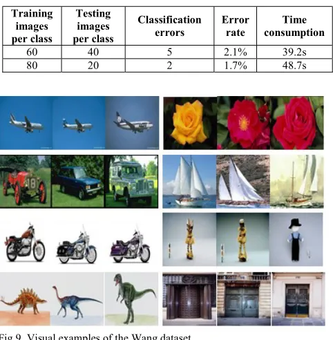
Fig.9. Visual examples of the Wang dataset
TABLEIV. IMAGE CLASSIFICATION RESULTS
Training images per class
Testing images per class
Classification
errors Error rate consumption Time
25 15 6 5% 30.6s
30 10 1 1.3% 34.5s
TABLEII. TIME CONSUMPTION FOR TRAINING (IN SECONDS)
Tr
ai
n
se
t
10
00
20
00
30
00
40
00
50
00
10
00
0
10
00
0(
2)
1
10
00
0(
4)
2
20
00
0
30
00
0
40
00
0
50
00
0
60
00
0
Ti
m
e
21
.4
41
.0
72
.3
11
3.
4
16
4.
5
52
7.
9
43
3.
7
39
0.
2
19
06
.8
39
75
.3
72
14
.9
10
67
2.
2
15
68
1.
7
1 2 local workers; 2 4 local workers.
and Hang clapping) with 100 images per class randomly extracted from 18 videos with the same background (3 videos per class). The visual examples of the images are presented in Fig. 8. In the experiments, the original images are converted to 64 64 size (2d64 ) because some of the actors are not large enough within the images. The experimental results are presented in Table III.
C. Image Classification
In this subsection, numerical examples with the proposed network for image classification are presented based on a subset of the Wang dataset [20]. The dataset used in this subsection consists of 8 classes with 40 images in each class. The 8 classes are: Airplanes, Cars, Dinosaur, Dolls, Doors, Motorbikes, Roses and Sailing ships. Example images of the 8 classes are given in Fig. 9. The original images are converted to 64 64 size and the experimental results are presented in Table IV.
D. Discussion
As it is shown in Table I and Fig. 6, the classification accuracy of the proposed network reaches 97.11% after all 60000 training images are used, which is slightly worse than the eClass1 and TEDAClass developed and published by our team earlier but outperform Neocognitron (and other approaches, i.e. neural networks, k-nearest neighbors classifiers [15]). One can also see that the performance of the proposed network keeps increasing if more training images are provided. In contrast, the eClass1 reaches its maximum accuracy after 40000 training images being processed. TEDAClass reaches its maximum accuracy after 30000 images being processed, with more training images, the accuracy of the TEDAClass decreases. For the proposed network, with more training samples and time consumptions, one can always obtain a higher accuracy.
Table II and Fig. 7 show that the training time consumption grows with the amount of training dataset. It only takes 113.4 seconds (using WIN10 OS and MATLAB and no parallelization) to train the network using 4000 images and the classification accuracy has already achieved over 95%, which by far, is the fastest training process among the established deep learning networks to the authors’ best knowledge. In additional, moving to Linux and C or Python can further speed up to an order of magnitude. For the published algorithms based on the global features (i.e. GIST and Haar), it already takes a larger amount of time (220.7 seconds) to only extract the GIST features from 4000 images. The Neocognitron neural network failed to
give us consistent result as the network has a large number of parameters and the training process for 5000 training images takes more than 5 hours [16], [18].
[image:7.612.315.556.406.652.2]the training process becomes much faster. It has to be stressed that, this parallelization experiments are not real parallel computation as all the training is still conducted within a single dual core PC. With more processers, or using GPUs, the training process will be even faster, and, critically, this algorithm allows parallelization at many levels.
Tables III and IV presented in sections V.B and V.C both demonstrate that the proposed network can be applied in different areas and is able to perform highly accurate classification results even if using a small amount of training images.
In summary, the numerical examples in section V clearly show the three advantages of the proposed network in addition to the advantage of interpretable features detailed in section IV: i) Fast, ii) highly accurate with increasing accuracy for more training samples and iii) Parallelizable.
VI. CONCLUSIONS
In this paper, a novel fast feedforward nonparametric deep learning network with automatic feature extraction is proposed. This new method is free from iterative parameter training and can learn from the training dataset very fast. In the learning stage, it automatically extracts the local aggregations from the training images and uses a nonlinear mapping function to improve their distinctiveness. The local area-based grid segmentation layer divides the extracted features into independent smaller sets that enables high level of parallelization. By selecting the most distinctive local aggregations, the network is able to build RBF neurons and further perform classification according to the Few-Winners-Take-All strategy. The advantages of the proposed network presented in this paper are as follows:
i) The extracted features are human understandable.
ii) No need for training of any parameters;
iii) The learning process is very fast;
iv) The learning process is fully parallelizable;
The numerical examples also illustrate that the proposed network is able to perform accurate classification for various problems.
VII. ACKNOWLEDGMENT
The authors would like to acknowledge the help of Dr. Dmitry Kangin in providing the comparative experimental results in Tables I and II.
REFERENCES
[1] D. Liu, D. Sun, and X. Zeng, “Recent Advances in Wavelength Selection Techniques for Hyperspectral Image Processing in the Food Industry,” Food Bioprocess Technol., vol. 7, pp. 307–323, 2014. [2] M. J. McAuliffe, F. M. Lalonde, D. McGarry, W. Gandler, K. Csaky,
and B. L. Trus, “Medical Image Processing, Analysis & Visualization
In Clinical Research,” in IEEE Symposium on Computer-Based
Medical Systems, 2001, pp. 381–386.
[3] T. H. Chen, K. L. Wu, and Y. C. Chiou, “An early fire-detection method based on image processing,” in International Conference on Image Processing, 2004, pp. 1707–1710.
[4] P. Angelov and P. Sadeghi-Tehran, “Look-a-Like: A Fast Content-Based Image Retrieval Approach Using a Hierarchically Nested Dynamically Evolving Image Clouds and Recursive Local Data Density,” Int. J. Intell. Syst., vol. 32, no. 1, pp. 82–103, 2016. [5] Y. LeCun, Y. Bengio, and G. Hinton, “Deep learning,” Nat. Methods,
vol. 13, no. 1, pp. 35–35, 2015.
[6] J. Ngiam, A. Khosla, M. Kim, J. Nam, H. Lee, and A. Y. Ng, “Multimodal Deep Learning,” Proc. 28th Int. Conf. Mach. Learn., pp. 689–696, 2011.
[7] A. Krizhevsky, I. Sutskever, and G. E. Hinton, “ImageNet Classification with Deep Convolutional Neural Networks,” Adv. Neural Inf. Process. Syst., pp. 1–9, 2012.
[8] D. Ciresan, U. Meier, and J. Schmidhuber, “Multi-column Deep Neural Networks for Image Classification,” Cvpr, pp. 3642–3649, 2012.
[9] K. Simonyan and A. Zisserman, “Very Deep Convolutional Networks for Large-Scale Image Recognition,” Int. Conf. Learn. Represent., pp. 1–14, 2015.
[10] D. C. Cireşan, U. Meier, L. M. Gambardella, and J. Schmidhuber, “Convolutional neural network committees for handwritten character classification,” Proc. Int. Conf. Doc. Anal. Recognition, ICDAR, vol. 10, pp. 1135–1139, 2011.
[11] J. Bruna and S. Mallat, “Invariant Scattering Convolution Networks,”
IEEE Trans. Pattern Anal. Mach. Intell., vol. 35, no. 8, pp. 1872–1886, 2013.
[12] F. A. Allah, W. I. Grosky, and D. Aboutajdine, “Document clustering based on diffusion maps and a comparison of the k-means performances in various spaces,” in IEEE Symposium on Computers and Communications, 2008, pp. 579–584.
[13] N. Dehak, R. Dehak, J. Glass, D. Reynolds, and P. Kenny, “Cosine Similarity Scoring without Score Normalization Techniques,” Proc. Odyssey 2010 - Speak. Lang. Recognit. Work. (Odyssey 2010), pp. 71– 75, 2010.
[14] X. Gu, P. P. Angelov, D. Kangin, and J. C. Principe, “A new type of distance metric and its application for NLP problems,” unpublished. [15] “MNIST Dataset,” http://yann.lecun.com/exdb/mnist/.
[16] K. Fukushima, “Neocognitron for handwritten digit recognition,”
Neurocomputing, vol. 51, pp. 161–180, 2003.
[17] P. Angelov and X. Zhou, “Evolving fuzzy-rule based classifiers from data streams,” IEEE Trans. Fuzzy Syst., vol. 16, no. 6, pp. 1462–1474, 2008.
[18] D. Kangin and P. Angelov, “Evolving clustering, classification and regression with TEDA,” in Proceedings of the International Joint Conference on Neural Networks, 2015, pp. 1–8.