Porto Institutional Repository
[Article] EEG Based Eye State Classification using Deep Belief Network and
Stacked AutoEncoder
Original Citation:
Narejo, Sanam; Pasero, Eros; Kulsoom, Farzana (2016).
EEG Based Eye State Classification using
Deep Belief Network and Stacked AutoEncoder.
In:
INTERNATIONAL JOURNAL OF ELECTRICAL
AND COMPUTER ENGINEERING
, vol. 6 n. 6, pp. 3131-3141. - ISSN 2088-8708
Availability:
This version is available at :
http://porto.polito.it/2655623/
since: November 2016
Publisher:
Institute of Advanced Engineering and Science (IAES)
Published version:
DOI:10.11591/ijece.v6i6.12967
Terms of use:
This article is made available under terms and conditions applicable to Open Access Policy Article
("["licenses_typename_cc_by_nc_nd_30_it" not defined]") , as described at
http://porto.polito.
it/terms_and_conditions.html
Porto, the institutional repository of the Politecnico di Torino, is provided by the University Library
and the IT-Services. The aim is to enable open access to all the world. Please
share with us
how
this access benefits you. Your story matters.
ISSN: 2088-8708, DOI: 10.11591/ijece.v6i6.12967 3131
EEG Based Eye State Classification using Deep Belief Network
and Stacked AutoEncoder
Sanam Narejo1, Eros Pasero2, Farzana Kulsoom3
1,2Department of Electronics & Telecommunications, Politecnico Di Torino, Italy 3Department of Electrical, Computer & Electronics, University of Pavia, Italy
Article Info ABSTRACT
Article history: Received Aug 14, 2016 Revised Oct 17, 2016 Accepted Nov 1, 2016
A Brain-Computer Interface (BCI) provides an alternative communication interface between the human brain and a computer. The Electroencephalogram (EEG) signals are acquired, processed and machine learning algorithms are further applied to extract useful information. During EEG acquisition, artifacts are induced due to involuntary eye movements or eye blink, casting adverse effects on system performance. The aim of this research is to predict eye states from EEG signals using Deep learning architectures and present improved classifier models. Recent studies reflect that Deep Neural Networks are trending state of the art Machine learning approaches. Therefore, the current work presents the implementation of Deep Belief Network (DBN) and Stacked AutoEncoders (SAE) as Classifiers with encouraging performance accuracy. One of the designed SAE models outperforms the performance of DBN and the models presented in existing research by an impressive error rate of 1.1% on the test set bearing accuracy of 98.9%. The findings in this study, may provide a contribution towards the state of the art performance on the problem of EEG based eye state classification.
Keyword: BCI
Deep belief networks Deep learning architectures Electroencephalogram Eye state classification Stacked autoencoders
Copyright © 2016 Institute of Advanced Engineering and Science. All rights reserved. Corresponding Author:
Sanam Narejo,
Department of Electronics and Telecommunication, Politecnico Di Torino, Italy.
Email: [email protected]
1. INTRODUCTION
Brain-Computer Interface (BCI) is one of the emerging fields in human computer interaction (HCI). It has a broad spectrum of solicitude; including safety-critical, security surveillance , industrial and medical applications. It has played a pivotal role in medical applications, for instance, patients with motor disabilities can alleviate communication abilities with aforesaid. BCI achieves this goal by establishing a connection path between stimulated brain and external device. BCIs are frequently aimed for research, mapping or repairing human cognitive or sensory-motor functions. In 1924 Berger was the first one to discover the electric activity of the human brain.
The electrical activity of the brain is recorded through Electroencephalography (EEG) in the form a signal. It can be also regarded as the recording of the brain's spontaneous electrical activity over a period of time. During acquisition, signals are obtained by applying several electrodes over scalp surface. However the position and number of electrodes are application and goal dependent. This electrical activity is then recorded in a form of signal. The signal obtained from EEG electrodes is processed in separate channel subsequently amplified. One may alternatively use the term channel or electrode [1].
A Principal aspect in the investigation of EEG signal is, the amount of information that can be acquired from the real EEG recordings. As stated earlier that in 1920s, the sensitivity of EEG to various changes of human brain’s functional state was demonstrated. It was also found in the above mentioned
studies that a simple action of closing the eyes, gives rise to regular oscillations in the EEG wave. Whereas during the conduct of any mental activity these oscillations become faster and less regular.
A significant challenge to an EEG based system, is the interference of artifacts in the signals. Artifacts are high frequency signals belong to non-cerebral origin and can dramatically alter the recorded signal. The artifacts are divided into two groups as internal and external. The external artifacts are generated from the environment or power equipments. The internal artifacts are eye blinks, eye movements, muscle and respiratory artifacts [2-3]. During the EEG experimental procedures, the subjects cannot control spontaneous eye movements or blinks [4]. These artifacts are almost inevitable, may seriously distort brain activity. Therefore, these occurrences establish the prominence of research on EEG, eye state signal analysis. Recently, the area of deep learning is attracting widespread interest by producing remarkable research in almost every aspect of artificial intelligence. Apart from achieving empirical success in the enormous number of practical applications, it has provided state of the art performance in natural language processing, speech recognition, object recognition and many other domains [5]. Deep learning has become one of the significant parts of the machine learning family. It is based on the set of algorithms that attempts to learn hierarchical, non linear representations of data. In a broader aspect this approach can also be termed as Representation learning. Learnt Representations often results in much better performance than can be obtained with hand-designed or hand-engineered representations for instance mathematical or statistical calculations [6]. Although all the deep learning approaches, share the idea of nested representation of data [7]. On the other hand, it is not always true that deep learning architectures may perform better than the shallow ones. Deeper architectures may lead, when there is sufficient amount of data to capture the patterns and the task is complex enough to be learnt through hierarchical multi-level non-linear transformations.
In this era, enormous research going on with the experiential and theoretical findings has brought Deep Learning Architectures (DLAs) to the attention of machine learning community. This paper presents the use of deep learning techniques to classify the state of the eye from EEG signals. This resulted as improved accuracy of predicting model over the conventional machine learning methods. The focus of our research is to implement deep learning architectures as classification models; specifically Deep Belief Network (DBN) and stacked AutoEncoder (SAE) and provide comparative analysis on the behavior and performance of SAE and DBF. Subsequently, comparing the obtained results with conventional Machine learning models of earlier studies. Deep learning is achieving state-of-the-art results across a range of difficult problem domains. To the best of our knowledge, this is the first application of Eye state prediction of EEG signals using deep architectures.
The rest of the manuscript is structured as follows. Section 2 provides the information on the related work for eye state classification, prediction or identification via EEG signals. Section 3 provides the brief overview of DLAs implemented in this research work. The details of the research methodology followed is explained in Section 4. Section 5 provides the vision on results and discussion. Section 6 deals with the conclusion and future work.
2. RELATED WORK
Eye state classification is a kind of common time series problem for detecting human cognitive state, which are not only crucial to medical care but also significant for daily life chores. There are various application areas related to the identification of the human cognitive state where EEG eye state classification task is the central element, such as epileptic seizure detection [8], stress feature identification [9], driving drowsiness detection [10], infant sleep-waking state identification [11]. Although some research work has already been done for eye state prediction, identification or detection in facial images and visual recordings too [12]. However, as illustrated in Introduction our aim is to predict the eye state from EEG signals as it causes deterioration in signal. Therefore, to foster this situation classification is done by deep learning architectures.
In the literature, researchers have attempted to successfully remove eye blink artifacts by de-veloping several methods for instance [13-15]. The authors in [16] provided the comparison of SVM and ANN for classification of EEG eye states such as, eye blink, eye open and eye closed. The SVM was justified as the preferred choice of model over ANN on the basis of performance accuracy given by both models. In addition, a hierarchical classification algorithm is developed using a thresholding method for offline recognition of four directions of eye movements from EEG signals [17].
The researchers in [18] proposed an EEG based eye tracking solution by using the information from two different sources, i.e., Head mounted Video-Oculuography and 16-channeled EEG signal. Their proposed model achieved the accuracy of 97.57% by extracting the features from source by using ICA rather than band-pass preprocessed EEG signals. A novel machine learning approach, incremental attribute learning
(IAL) is proposed in [19] for EEG eye state time series classification. The IAL algorithm progressively imports and trains features one at a time to predict the class labeling.
In [20], the researchers have studied the differences among three states, i.e. Eye-closed, Eye-open and Attension states of human using EEG signals. The major goal of their research was to address the issue of how spatial-temporal properties of alpha rhymes were affected by the change of human brain state. However, the authors did not pursue further towards the predictive model for the classification task of the above mentioned states.
The researchers developed EEG Eye state corpus and tested 42 different classifiers for detecting whether an individual's eyes are open or closed based on EEG recordings [21]. It was explored that k* algorithm achieved the highest accuracy in comparison with others, achieving the correct classification rate of 97.3%. Their developed Eye state corpus is now stored in the Machine learning repository as a benchmark problem [22]. The same corpus is further used in [23] as time series classification task based on IAL approach, with the Feature ordering based on Accumulative Discriminability (AD).
The study of Oliver Roesler and David Suendermann [21] is further extended in [24] in which three different ensemble learning models are developed and the accuracy achieved with the most accurate model constructed from Regularized Random Forest RRF and K* is 97.4 %. The research work in [25] proposed a novel system based on small numbers of Neuro Fuzzy rules for similar classification problem. In their study, weight parameter tunning was done by adjusting the standard deviations. The best possible results were achieved by tuning the parameters asymmetrically through test cases with the average error rate of 4.0%.
3. THE COMPREHENSIVE THEORY
The DLAs are comprised of multiple levels of non-linear operations, like neural networks with several hidden layers. The standard training strategy of neural network and the gradient based optimization, often gets stuck in local minima and finds the poor solution for the network with multiple hidden layers. Intuitively, it is difficult to train deep neural networks with standard learning algorithms because searching the parameter space becomes difficult in deeper networks. This issue gets resolved by initializing the weight parameters of deep neural network through greedy layer wise unsupervised training as introduced in [26-28].
3.1. Deep Belief Network
DBN holds a great promise as a principle to address the problem of training deep neural networks. DBN are composed of multiple layers of stochastic, unsupervised model such as Restricted Boltzmann Machines (RBMs), which are used to initialize the network in the region of parameter space that finds good minima of the supervised objective.
RBMs are probabilistic graphical models that are connected bi-directionally and can be inferred as stochastic neural networks. RBM relies on two layer structure comprising on visible and hidden nodes, this concept is shown in Figure 1. The visible units constitute the first layer and correspond to the components of an observation where as the hidden units model dependencies between the components of observations. The RBM is trained to model the joint probability distribution of inputs or explanatory variables and the corresponding labels or response variables, both represented by the visible units of the RBM. The probabilities of both hidden and visible nodes are expressed in equation (1).
( | ) ∏ ( | ) ( | ) ∏ ( | ) (1) The conditional probability of a single variable to be 1, can be then interpreted as the firing rate of a stochastic neuron with sigmoid activation function σ(x) = 1/(1 + e^(-x)). Therefore the binary states of hidden units and reconstruction from those hidden units as visible nodes in above equations can be further interpreted in form of equations (2) and (3) as
( | ) (∑ ) (2) ( | ) (∑ ) (3) Where, Wij is the weight associated between the units vj and hi whereas bj and ci are the bias terms. The change in a weight parameter is then given by (4).
The idea is that the hidden neurons extract relevant features from the observations. These features serve as input to another RBM. By stacking RBMs in this way, one can achieve high level representations by learning the features from features.
DBNs are capable of extracting a deep hierarchical representation of the training data. The top layers of DBN are responsible as a source of more “abstract and meaningful” representations that explain the input observation x, whereas lower layer extracts “low level features”.
Figure. 1. The structure of a single RBM composed of visible layer and hidden layer
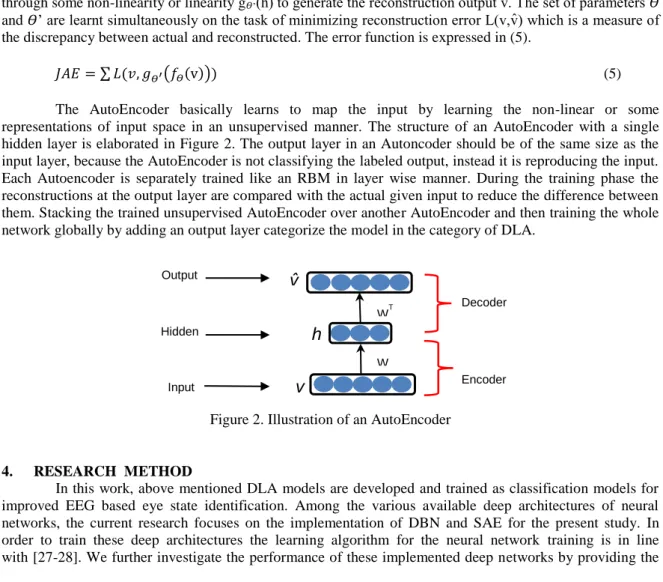
3.2. Stacked AutoEncoder
An alternative approach to deep learning is Stacked Autoencoder, where the hidden units generate exploitable numeric feature values. As demonstrated in [29-30] AutoEncoders have become the dominant focal point in the area of “deep architectures”. An AutoEncoder is a neural network that consists of two parts: encoder and decoder. It is trained in such a way to reconstruct the given input at the output layer. The first part, the encoder is responsible to compute the hidden representations h of input space v through some nonlinear transfer function f(v). The decoder takes these latents produced by encoders and further passes it through some non-linearity or linearity g𝛳’(h) to generate the reconstruction output v . he set of parameters 𝛳 and 𝛳’ are learnt simultaneously on the task of minimizing reconstruction error (v,v ) which is a measure of the discrepancy between actual and reconstructed. The error function is expressed in (5).
∑ ( ( ( ))) (5) The AutoEncoder basically learns to map the input by learning the non-linear or some representations of input space in an unsupervised manner. The structure of an AutoEncoder with a single hidden layer is elaborated in Figure 2. The output layer in an Autoncoder should be of the same size as the input layer, because the AutoEncoder is not classifying the labeled output, instead it is reproducing the input. Each Autoencoder is separately trained like an RBM in layer wise manner. During the training phase the reconstructions at the output layer are compared with the actual given input to reduce the difference between them. Stacking the trained unsupervised AutoEncoder over another AutoEncoder and then training the whole network globally by adding an output layer categorize the model in the category of DLA.
Figure 2. Illustration of an AutoEncoder
4. RESEARCH METHOD
In this work, above mentioned DLA models are developed and trained as classification models for improved EEG based eye state identification. Among the various available deep architectures of neural networks, the current research focuses on the implementation of DBN and SAE for the present study. In order to train these deep architectures the learning algorithm for the neural network training is in line with [27-28]. We further investigate the performance of these implemented deep networks by providing the
W WT Decoder Encoder Hidden Input Output
h
v
v̂
comparative analysis with each other and with some of other conventional machine learning approaches mentioned in the subsequent section. A distinguishable factor of the deep learning architectures from conventional classifiers is the automatic feature learning from data which mainly contributes to improvement in the accuracy of the model. Apart from this the deep learning algorithms introduced recently, solves the hard optimization problem into several greedy steps, though the simple ones, to train the deeper networks.
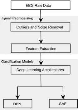
The research strategy followed in this work is demonstrated in Figure 3. Initially, the data is pre-processed by removing the noise or any kind of an outlier. Afterwards, the meaningful feature set is formed by applying the DWT transformation on EEG signal as explained in the later part of this section. Before presenting the extracted feature set to the classification models for training, the feature set was normalized in the range of (0,1) so that the network learns efficiently. Finally the preprocessed dataset was used for the training of classification models. For classification models, as we explained earlier, our major focus is to explore the performance of DBN and SAE. The major objective was, the lowest possible error and high accuracy to be achieved by implemented models. Hence, the training of Deep Architectures took a couple of days, which was not the most important target for our case. The detail explanation of the steps followed are specified below.
The EEG data set was taken from the UCI machine Learning repository, which is a benchmark for the Eye state classification problem. The EEG signal was recorded from 14 different electrodes with the Emotiv EEG Neuroheadset. The eye state either open or closed was captured manually by means of a camera during the EEG measurement and the captured frames were interpreted as 1 and 0 in correspond to Eye-closed and Eye-open states. The duration of the measurement was 117 seconds with 14980 samples. The EEG signal was further preprocessed for outliers and noise.
Figure 3. Flow of Research Methodology
In order to extract useful features from EEG time series signal Discrete Wavelet Transform (DWT) was applied. In the domain of biomedical signals DWT has been widely used for time-frequency analysis [31]. Traditionally used Short term Fourier transforms perform temporal resolution and highlight change in spectrum with respect to time. On the other hand it gives a uniform resolution in the frequency domain. The wavelet transform provides a window that has a constant relative error in the frequency domain, rather than constant absolute error, at the expense of time resolution, in accordance with Heisenberg's uncertainty principle. Multi level Wavelet decomposition resolves the major wavelet into different frequency bands alpha, beta, gamma, delta, theta and sigma.
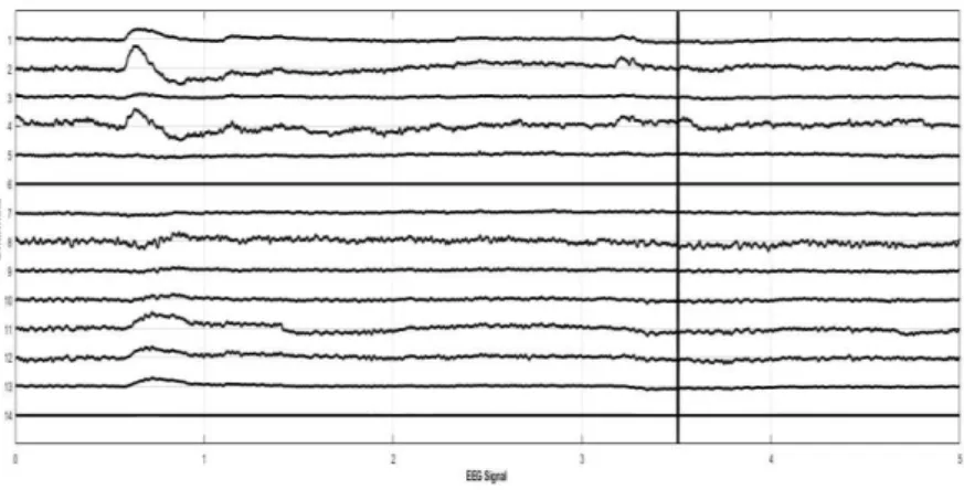
As we have specified earlier, the EEG data set used in this study contains signals from 14 different electrodes. The 14 electrodes are considered as 14 different channels as shown in the Figure 4 and DWT is applied to the signal of each channel.
Signal Preprocessing
Classification Models
EEG Raw Data
Feature Extraction Outliers and Noise Removal
Deep Learning Architectures
Figure 4. EEG Signals Generated from 14 Electrodes
The DWT decompositions of signals are actually the outcomes of high pass and low pass filtering. The approximations are the high-scale, low-frequency components of the signal. The details are the low-scale, high-frequency components. The EEG signal is further decomposed into level 8 Approximations a8 and Details d1-d8. The level of decomposition depends on the principal frequency components. Figure 5 indicates the phenomena of 4 level DWT decomposition tree. These decompositions termed as subband features are often used as an input feature set of attributes for various classification and prediction tasks [32].
For each channel signal separate decompositions were computed. Subsequently, the frequency bands alpha, beta, gamma, theta and delta are estimated from those computed decompositions. In this way, each signal from each channel is presented in terms of the above mentioned five bands. Therefore the feature set consists of total 14 multiplied by 5 as total attributes. The normalization procedure was further applied on the feature set to bring the values in the range between 0 and 1.
Figure 5. Presentation of 4-level DWT Decomposition Tree
In this part of work, experiments are presented to analyze and explore the deep learning architectures that falls in two broad and major categories i.e. DBN and SAE and to further investigate the performance of both models on the basis of comparative analysis.
4.1. Experimental Setup 1
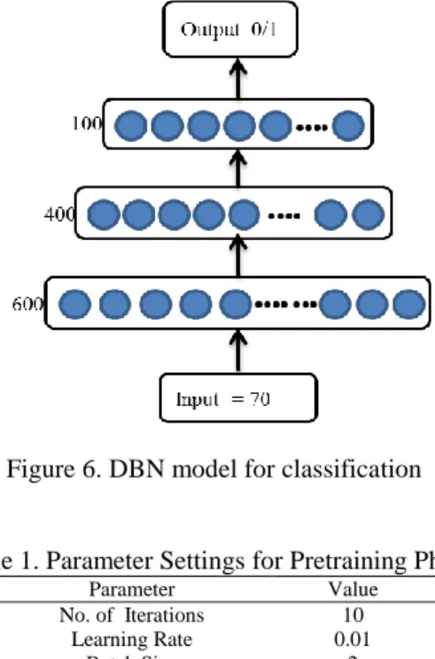
In this step, DBN model was developed and trained. The network model was formed by stacking the RBMs. A DBN was developed with an input layer consisting of 70 units, three hidden layers of size (600-400-100) and an output layer with one unit to predict the class of an EEG signal i.e. open or close. The ultimate architecture of the trained DBN model is shown in Figure 6. To select the topological structure of the hidden layers of DBN the demonstrations given in [33] were followed. Each layer of the DBN is independently trained as an RBM with the Sigmoid activation function. The states of hidden nodes determined by trained RBM were used as input to the next layer. After unsupervised training, the labels of
EEG Eye events were provided at the output layer for linear mapping. The preferred parameter selections for the pretraining of DBN are revealed in Table 1.
Figure 6. DBN model for classification
Table 1. Parameter Settings for Pretraining Phase
Parameter Value
No. of Iterations 10
Learning Rate 0.01
Batch Size 2
Transfer Function Sigmoid
Once the layers of RBM in DBN were trained, an output layer with Cross Entropy cost function was added. In this way, the network was globally fine tuned with a supervised algorithm to predict the targets. The total 600 iterations were implemented to train the network with the added linear output layer.
4.2. Experimental Setup 2
Stacked Autoencoders as DLA exist in several forms of variations [7]. In this study, we attempt to implement the sparse AutoEncoders. In the primary step, to find the accurate model, several numbers of models as sparse SAE were developed and trained. Initially, these neural networks were designed for the goal of dimensionality reduction, but, with the growing fame of Representation Learning the dimensions do not necessarily need to be lower than the input size. However, there exists a problem if the hidden layers of an AutoEncoder are either allowed too much capacity or hold insufficient dimensions. The AutoEncoder attempts to replication task, instead of learning the internal representation of input distribution and extracting the useful information, it works as an identity function. The provision for this issue is a Regularize Autoencoder. Rather than constraining the hidden layer dimensions or model capacity regularized AutoEncoder are sparse and uses a loss function with some sparsity penalty as expressed in (6).
∑ ( ( ( ))) ( ) ( )
(6)
Since our focus was to choose the models with the best classification ability, therefore only selected SAE models are included here for further discussion. Table 2 demonstrates the selected ones from various implemented SAE models along with their parameter specifications. The sparsity proportion is a parameter of sparsity regulerizer which must be selected in the range of 0 to 1, whereas λ and β are the coefficients to 2 weight regularization and sparsity regularization. Detailed discussion on model accuracy and performance is provided in the next section.
Table 2. Parameter Settings for Pretraining Phase
SAE models Architecture
Hidden Layer Parameters Output layer
β λ Sparsity Proportion Activation Function Activation Function SAE 1 70-100-200-2 3 0.001 0.05 Encoder=logsig Decoder=purelin Softmax SAE 2 70-200-100-2 3 0.001 0.05 SAE 3 70-500-200-2 3 0.001 0.05 SAE 4 70-600-200-2 3 0.001 0.05 SAE 5 70-100-100-2 1 0.01 0.05 SAE 6 70-200-100-2 4 0.001 0.06
5. RESULTS AND DISCUSSION
As intimated earlier, the emphasis of this research study was to formulate the improved EEG based eye state classification task using two different paradigms of deep neural networks and to further improve the state of the art performance. In response to conduct this, the DBN and SAE were preferred cardinal models as deep learning architectures. For this purpose, the data source was the benchmark data set of EEG eye state classification time series available online [22]. The results achieved here are noticeably encouraging and evidenced to be better in most of the cases than the earlier results reported for EEG eye state classification problem.
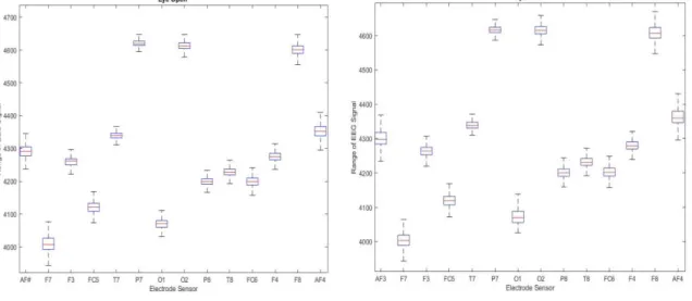
The boxplot is drawn separately for each class as presented in Figures 7(a) and (b) in order to study the distributional characteristics of a 14-channelled EEG signal. The boxplot is a useful way to visualize the range and other statistical characteristics of response variables. It is obvious from the figures that there is a higher value of difference when the signal amplitude from certain sensors is compared.
It is apparent from various studies that a deep learning algorithm greatly reduces the error on test sets due to its strong unsupervised learning phase. Apart from this, unsupervised pretraining behaves as a kind of data dependent regularizer to avoid overfitting criteria. It is an undeniable fact that unsupervised pretraining being injected as local layerwise training, extracts the salient information about the input distribution and the essence of nonlinear structure present in the data. The interpretations attained in this study are consistent and correlated with the earlier studies conducted in the realm of deeper NN architectures.
Figure 7(a). Statistical Range of Electrode Signals for Eye Open, (b) Statistical Range of Electrode Signals for Eye Close
In order to distinguish the best deep learning models from among those implemented for the EEG based eye state classification task, the comparative analysis was performed for a few of the trained models, summarized in Table 3. This was based on the classifier’s performance and misclassification rate as averaged error on test sets. The performance of each classifier was computed using the most commonly used parameters: accuracy, sensitivity and specivity. Accuracy was calculated as expressed by the (7). Sensitivity
and specificity are statistical measures of the performance as expressed by the equations (8) and (9) respectively.
Accuracy=Total No. of Samples Classified Correctly /Total No. of Samples (7)
Sensitivity=TP/TP+FN (8)
Specificity=TN/TN+FP (9)
Table 3. Parameter Settings for Pretraining Phase
It is evident from the Table 3 that both the DBN and SAE models accomplished higher prediction accuracy and are almost compatible. In comparison with conventional Machine learning models, the deep learning approach based on unsupervised pre training and supervised fine tuning provides a better generalization than the supervised learning models with random initializations. The random initializations for the parameters of a neural network, declare the parameters in regions of the parameter space that generalize poorly. As mentioned earlier, only a few developed models are selected and included in this article for discussion. It is obvious from the experimental consequences that the quantitative analysis is almost similar with only slight differences.
One of the superlative SAE models i.e SAE 2 inclined to provide the accuracy of 98.9 %, which is evidently higher than the rest of the other models performance. It also appears that the applied approach of developing SAE 2 outperforms the DBN model with the difference of 1.1% except of the two cases. The constraints in SAE models experiment applied to the optimization procedure enforced the model to capture not only the input to target dependency, but also the statistical regularities of the input distribution which resulted in prominently better performance than DBN.
The two exceptional cases as mentioned earlier include, model SAE 5 and SAE 6. The tuning parameters in these models, consisting of coefficients for sparsity and L2 regularization, are different from the other SAE models as presented in Table 2. Contextually, this resulted in considerably lower performance as compared to the other developed SAE models. On the other hand, to enforce the classifier to predict well, the selection of sufficient hidden layer dimension in deeper architecture is another critical point to consider. To avoid electing the hidden layer sizes arbitrarily, the comprehensive strategy to follow is well explained in [33]. In addition to this some effort must be logically done while investigating the several possibilities for the dimension of hidden layers. During the training procedure, it was also found that in the deeper hierarchical structure of the network, when performing the Representation Learning or feature extraction, the model learns the simple concepts at lower layer levels and more abstract concept are learnt by composing them at higher top layers of the network.
Table 4. Comparison with Previous Research
Models Accuracy Error Rate
Proposed DLA model, SAE 2 98.9 % 1.1%
K*+RRF [24] 97.4 % 2.6%
K* [21] 97.3% 2.7%
Neuro-Fuzzy[25] 96% 4.0%
Table 4 highlights the accomplishment of our best classifier i.e SAE 2. The researchers in [21], demonstrated the performance analysis of 42 classifiers on the problem of Eye state classification through EEG signal. Among all of those trained classifiers, K* was found to be the most promising one with an accuracy of 97.30%. However, afterwards the authors in [24] extended the aforementioned work by proposing an ensemble classifier with a better performance of around 97.40 % accuracy. Meanwhile the
Deep Architectures Specitivity Sensitivity Accuracy Error rate
DBN 0.99 0.89 97.1% 2.9% SAE 1 0.95 0.98 97.6% 2.4% SAE 2 0.96 0.99 98.9% 1.1% SAE 3 0.94 0.99 97.8% 2.2% SAE 4 0.94 0.99 97.8% 2.2% SAE 5 0.80 0.97 92.9% 7.1% SAE 6 0.74 0.99 91.9% 8.8%
researchers trained a Neuro-Fuzzy classifier which gave the performance accuracy around 96%. In contrast to the above mentioned studies, the proposed SAE 2 model trained with the specified procedure and parameter settings outperforms other models, with the obtained error rate of only 1.1% on the test set. Higher accuracy, around 98.9 %, is accomplished on the test samples which demonstrates improved performance over [21], [24] and [25]. We hypothesize that there is a possibility of achieving much better results through deep architectures by implementing Denoising and Contrastive Autoencoders. This indicates a direction for possible future work to further extend this study.
6. CONCLUSION
The directed research focuses on two approaches of DLA for EEG Eye state classification task as eye open or close. Although this has been done earlier in a number of ways with different Machine learning classifiers, albeit our endeavor improves on the classification accuracy by applying deep architectures as classifiers. Several numbers of models were trained for the study and some of them are presented in this article for significant discussion. A straightforward analysis procedure has been conducted on the basis of different performance measurement metrics. Our trained models with the hyperparameter settings and applied hidden layer dimensions achieved striking performances as compared to the existing ones. Most notably, to our knowledge, this is the first study of EEG based eye state classification tasks using deep Neural Network models, i.e., DBN and SAE. The study conducted here can be applied in different application domains of BCI and for the identification of human cognition. Most imperatively where the artifacts generated by eye movements or eye blinks are crucial, there is a need for them to be identified and further removed.
ACKNOWLEDGEMENTS
This research activity was partly funded by Italian MIUR OPLON project and supported by the Politecnico of Turin NEC NEURONICA laboratory. Computational resources were partly provided by HPC@POLITO, (http://www.hpc.polito.it).
REFERENCES
[1] Kaplan A. Y. and Shishkin S. L., “Application of the change-point analysis to the investigation of the brain’s electrical activity,” in Non-parametric statistical diagnosis, Springer Netherlands, pp. 333-388, 2000.
[2] Teplan M., “Fundamentals of EEG measurement,” Measurement science review, vol/issue: 2(2), pp. 1-1, 2002. [3] J. Zhang and V. L. Patel, “Distributed cognition, representation, and affordance,” Pragmatics & Cognition,
vol/issue: 14(2), pp. 333-341, 2006.
[4] Hoffmann S. and Falkenstein M., “The correction of eye blink artefacts in the EEG: a comparison of two prominent methods. PLoS One, vol/issue: 3(8), pp. e3004, 2008.
[5] L. Cun, et al., “Deep learning,” Nature, vol/issue: 521(7553), pp. 436-444, 2015.
[6] Bengio Y., et al., “Representation learning: A review and new perspectives,” IEEE transactions on pattern analysis and machine intelligence, vol/issue: 35(8), pp. 1798-828, 2013.
[7] I. Goodfellow, et al., “Deep Learning,” Book in preparation for MIT Press, 2016.
[8] Polat K. and Güneş S., “Classification of epileptiform EEG using a hybrid system based on decision tree classifier and fast Fourier transform,” Applied Mathematics and Computation, vol/issue: 187(2), pp. 1017-26, 2007.
[9] Sulaiman N., et al., “Novel methods for stress features identification using EEG signals,” International Journal of Simulation: Systems, Science and Technology, vol/issue: 12(1), pp. 27-33, 2011.
[10] Yeo M. V., et al., “Can SVM be used for automatic EEG detection of drowsiness during car driving?” Safety Science, vol/issue: 47(1), pp. 115-24, 2009.
[11] Estévez P. A., et al., “Polysomnographic pattern recognition for automated classification of sleep-waking states in infants,” Medical and Biological Engineering and Computing, vol/issue: 40(1), pp. 105-13, 2002.
[12] Cheng E., et al., “Eye state detection in facial image based on linear prediction error of wavelet coefficients,” in
Robotics and Biomimetics, 2008. ROBIO 2008. IEEE International Conference, pp. 1388-1392, 2009.
[13] G. Gratton, et al., “A new method for off-line removal of ocular artifact,” Electroencephalography and clinical neurophysiology, vol/issue: 55(4), pp. 468-484, 1983.
[14] Shoker L., et al., “Removal of eye blinking artifacts from EEG incorporating a new constrained BSS algorithm,” in
Sensor Array and Multichannel Signal Processing Workshop Proceedings, pp. 177-181, 2004.
[15] Krishnaveni V., et al., “Removal of ocular artifacts from EEG using adaptive thresholding of wavelet coefficients,”
Journal of Neural Engineering, vol/issue: 3(4), pp. 338, 2006.
[16] Singla R., et al., “Comparison of SVM and ANN for classification of eye events in EEG,” Journal of Biomedical Science and Engineering, vol/issue: 4(01), pp. 62, 2011.
[17] Belkacem A. N., et al., “Classification of four eye directions from EEG signals for eye-movement-based communication systems,” life, vol. 1, pp. 3, 2014.
[18] Samadi M. R. and Cooke N., “EEG signal processing for eye tracking,” in 2014 22nd European Signal Processing Conference (EUSIPCO), pp. 2030-2034, 2014.
[19] Wang T., et al., “EEG eye state identification using incremental attribute learning with time-series classification,”
Mathematical Problems in Engineering, 2014.
[20] Li L., “The differences among eyes-closed, eyes-open and attention states: an EEG study,” in 2010 6th International Conference on Wireless Communications Networking and Mobile Computing, pp. 1-4, 2010.
[21] O. Rösler and D. Suendermann, “A first step towards eye state prediction using eeg,” Proc. of the AIHLS, 2013. [22] A. Frank and A. Asuncion, “UCI machine learning repository,” 2010.
[23] Wang T., et al., “Time series classification for EEG eye state identification based on incremental attribute learning,” in Computer, Consumer and Control (IS3C), 2014 International Symposium, pp. 158-161, 2014. [24] Hamilton C. R., et al.,“Eye State Prediction from EEG Data Using Boosted Rotational Forests,” in 2015 IEEE 14th
International Conference on Machine Learning and Applications (ICMLA), pp. 429-432, 2015.
[25] Y. M. Kim, et al., “Computing Intelligence Approach for an Eye State Classification with EEG Signal in BCI,”
Software Engineering and Information Technology: Proceedings of the 2015 International Conference on Software Engineering and Information Technology (SEIT2015). World Scientific, 2015.
[26] Hinton G. E., et al., “A fast learning algorithm for deep belief nets,” Neural computation, vol/issue: 18(7), pp. 1527-54, 2006.
[27] Bengio Y., et al., “Greedy layer-wise training of deep networks,” Advances in neural information processing systems, vol. 19, pp. 153, 2007.
[28] Salakhutdinov R. and Hinton G. E., “Deep Boltzmann Machines,” in AISTATS, vol. 1, pp. 3, 2009.
[29] G. E. Hinton and R. R. Salakhutdinov, “Reducing the dimensionality of data with neural networks,” Science,
vol/issue: 313(5786), pp. 504-507, 2006.
[30] Erhan D., et al., “Why does unsupervised pre-training help deep learning?” Journal of Machine Learning Research, pp. 625-60, 2010.
[31] Aowlad A. B., et al., “Left and Right Hand Movements EEG Signals Classification Using Wavelet Transform and Probabilistic Neural Network,” International Journal of Electrical and Computer Engineering, vol/issue: 5(1), pp. 92, 2015.
[32] Megat M. S., et al., “Learning Style Classification via EEG Sub-band Spectral Centroid Frequency Features,”
International Journal of Electrical and Computer Engineering, vol/issue: 4(6), pp. 931, 2014.
[33] Larochelle H., et al., “Exploring strategies for training deep neural networks,” Journal of Machine Learning Research, pp. 1-40, 2009.
BIOGRAPHIES OF AUTHORS
Sanam Narejo is a PhD student at the Department of Electronics and Telecommunications (DET), Politecnico Di Torino, Italy. She is doing her research under the supervision of Professor Eros Pasero. She received her M.Sc degree in Communication Systems and Networking from Mehran University of Engineering and Technology (MUET) in 2012. Her research interests include Signal Processing, Artificial Neural Networks and Deep Learning Architectures.
Eros Pasero is Professor at the Department of Electronics and Telecommunication (DET), Politecnico Di orino, Italy since 1991. He is the founder of “Neuronica ab”, a laboratory for research and development of neural networks. His interests lie in Artificial Neural Networks and Electronic Sensors. He is the President of SIREN, the Italian Society for Neural Networks. He has supervised more than tenths of international Ph.D students and hundredths of Master students. He holds 5 international patents. He is author of more than 100 international publications.
Farzana Kulsoom is a profound researcher in signal processing and enthusiastic educatinst. She is a PhD student at University of Pavia, Italy. She has done B.Sc in Computer Engineering in 2006 and M.Sc in Telecommunication Engineering in 2012 at UET, Taxila Pakistan.